Thuật toán và cấu trúc dữ liệu
Bạn đang xem bản rút gọn của tài liệu. Xem và tải ngay bản đầy đủ của tài liệu tại đây (2.03 MB, 305 trang )
Algorithms and Data Structures
Kurt Mehlhorn
•
Peter Sanders
Algorithms and
Data Structures
The Basic Toolbox
Prof. Dr. Kurt Mehlhorn Prof. Dr. Peter Sanders
Max-Planck-Institut für Informatik Universität Karlsruhe
Saarbrücken Germany
Germany
ISBN 978-3-540-77977-3 e-ISBN 978-3-540-77978-0
DOI 10.1007/978-3-540-77978-0
Library of Congress Control Number: 2008926816
ACM Computing Classification (1998): F.2, E.1, E.2, G.2, B.2, D.1, I.2.8
c
2008 Springer-Verlag Berlin Heidelberg
This work is subject to copyright. All rights are reserved, whether the whole or part of the material is
concerned, specifically the rights of translation, reprinting, reuse of illustrations, recitation, broadcasting,
reproduction on microfilm or in any other way, and storage in data banks. Duplication of this publication
or parts thereof is permitted only under the provisions of the German Copyright Law of September 9,
1965, in its current version, and permission for use must always be obtained from Springer. Violations are
liable to prosecution under the German Copyright Law.
The use of general descriptive names, registered names, trademarks, etc. in this publication does not
imply, even in the absence of a specific statement, that such names are exempt from the relevant protective
laws and regulations and therefore free for general use.
Cover design: KünkelLopka GmbH, Heidelberg
Printed on acid-free paper
987654321
springer.com
To all algorithmicists
Preface
Algorithms are at the heart of every nontrivial computer application. Therefore every
computer scientist and every professional programmer should know about the basic
algorithmic toolbox: structures that allow efficient organization and retrieval of data,
frequently used algorithms, and generic techniques for modeling, understanding, and
solving algorithmic problems.
This book is a concise introduction to this basic toolbox, intended for students
and professionals familiar with programming and basic mathematical language. We
have used the book in undergraduate courses on algorithmics. In our graduate-level
courses, we make most of the book a prerequisite, and concentrate on the starred
sections and the more advanced material. We believe that, even for undergraduates,
a concise yet clear and simple presentation makes material more accessible, as long
as it includes examples, pictures, informal explanations, exercises, and some linkage
to the real world.
Most chapters have the same basic structure. We begin by discussing a problem
as it occurs in a real-life situation. We illustrate the most important applications and
then introduce simple solutions as informally as possible and as formally as neces-
sary to really understand the issues at hand. When we move to more advanced and
optional issues, this approach gradually leads to a more mathematical treatment, in-
cluding theorems and proofs. This way, the book should work for readers with a wide
range of mathematical expertise. There are also advanced sections (marked with a *)
where we recommend that readers should skip them on first reading. Exercises pro-
vide additional examples, alternative approaches and opportunities to think about the
problems. It is highly recommended to take a look at the exercises even if there is
no time to solve them during the first reading. In order to be able to concentrate on
ideas rather than programming details, we use pictures, words, and high-level pseu-
docode to explain our algorithms. A section “implementation notes” links these ab-
stract ideas to clean, efficient implementations in real programming languages such
as C
++
and Java. Each chapter ends with a section on further findings that provides
a glimpse at the state of the art, generalizations, and advanced solutions.
Algorithmics is a modern and active area of computer science, even at the level
of the basic toolbox. We have made sure that we present algorithms in a modern
VIII Preface
way, including explicitly formulated invariants. We also discuss recent trends, such
as algorithm engineering, memory hierarchies, algorithm libraries, and certifying
algorithms.
We have chosen to organize most of the material by problem domain and not by
solution technique. The final chapter on optimization techniques is an exception. We
find that presentation by problem domain allows a more concise presentation. How-
ever, it is also important that readers and students obtain a good grasp of the available
techniques. Therefore, we have structured the final chapter by techniques, and an ex-
tensive index provides cross-references between different applications of the same
technique. Bold page numbers in the Index indicate the pages where concepts are
defined.
Karlsruhe, Saarbrücken, Kurt Mehlhorn
February, 2008 Peter Sanders
Contents
1 Appetizer: Integer Arithmetics 1
1.1 Addition . . . . . . . . . . . . . . . . . . . . . . . . . . . . . . . . . . . . . . . . . . . . . . . . . 2
1.2 Multiplication: The School Method . . . . . . . . . . . . . . . . . . . . . . . . . . 3
1.3 Result Checking . . . . . . . . . . . . . . . . . . . . . . . . . . . . . . . . . . . . . . . . . . 6
1.4 A Recursive Version of the School Method . . . . . . . . . . . . . . . . . . . . 7
1.5 Karatsuba Multiplication . . . . . . . . . . . . . . . . . . . . . . . . . . . . . . . . . . . 9
1.6 Algorithm Engineering . . . . . . . . . . . . . . . . . . . . . . . . . . . . . . . . . . . . . 11
1.7 ThePrograms 13
1.8 Proofs of Lemma 1.5 and Theorem 1.7 . . . . . . . . . . . . . . . . . . . . . . . 16
1.9 ImplementationNotes 17
1.10 Historical Notes and Further Findings . . . . . . . . . . . . . . . . . . . . . . . . 18
2 Introduction 19
2.1 AsymptoticNotation 20
2.2 The Machine Model . . . . . . . . . . . . . . . . . . . . . . . . . . . . . . . . . . . . . . . 23
2.3 Pseudocode . . . . . . . . . . . . . . . . . . . . . . . . . . . . . . . . . . . . . . . . . . . . . . 26
2.4 Designing Correct Algorithms and Programs . . . . . . . . . . . . . . . . . . 31
2.5 An Example – Binary Search 34
2.6 BasicAlgorithmAnalysis 36
2.7 Average-Case Analysis . . . . . . . . . . . . . . . . . . . . . . . . . . . . . . . . . . . . . 41
2.8 Randomized Algorithms. . . . . . . . . . . . . . . . . . . . . . . . . . . . . . . . . . . . 45
2.9 Graphs . . . . . . . . . . . . . . . . . . . . . . . . . . . . . . . . . . . . . . . . . . . . . . . . . . 49
2.10 P and NP 53
2.11 ImplementationNotes 56
2.12 Historical Notes and Further Findings . . . . . . . . . . . . . . . . . . . . . . . . 57
3 Representing Sequences by Arrays and Linked Lists 59
3.1 LinkedLists 60
3.2 Unbounded Arrays . . . . . . . . . . . . . . . . . . . . . . . . . . . . . . . . . . . . . . . . 66
3.3 *AmortizedAnalysis 71
3.4 Stacks and Queues . . . . . . . . . . . . . . . . . . . . . . . . . . . . . . . . . . . . . . . . 74
X Contents
3.5 ListsVersusArrays 77
3.6 ImplementationNotes 78
3.7 Historical Notes and Further Findings . . . . . . . . . . . . . . . . . . . . . . . . 79
4 Hash Tables and Associative Arrays 81
4.1 HashingwithChaining 83
4.2 UniversalHashing 85
4.3 Hashing with Linear Probing . . . . . . . . . . . . . . . . . . . . . . . . . . . . . . . . 90
4.4 Chaining Versus Linear Probing . . . . . . . . . . . . . . . . . . . . . . . . . . . . . 92
4.5 *PerfectHashing 92
4.6 ImplementationNotes 95
4.7 Historical Notes and Further Findings . . . . . . . . . . . . . . . . . . . . . . . . 97
5 Sorting and Selection 99
5.1 SimpleSorters 101
5.2 Mergesort – an O(nlogn) SortingAlgorithm 103
5.3 A Lower Bound . . . . . . . . . . . . . . . . . . . . . . . . . . . . . . . . . . . . . . . . . . . 106
5.4 Quicksort 108
5.5 Selection 114
5.6 Breaking the Lower Bound . . . . . . . . . . . . . . . . . . . . . . . . . . . . . . . . . 116
5.7 *ExternalSorting 118
5.8 ImplementationNotes 122
5.9 Historical Notes and Further Findings . . . . . . . . . . . . . . . . . . . . . . . . 124
6 Priority Queues 127
6.1 Binary Heaps . . . . . . . . . . . . . . . . . . . . . . . . . . . . . . . . . . . . . . . . . . . . . 129
6.2 Addressable Priority Queues . . . . . . . . . . . . . . . . . . . . . . . . . . . . . . . . 133
6.3 *ExternalMemory 139
6.4 ImplementationNotes 141
6.5 Historical Notes and Further Findings . . . . . . . . . . . . . . . . . . . . . . . . 142
7 Sorted Sequences 145
7.1 Binary Search Trees . . . . . . . . . . . . . . . . . . . . . . . . . . . . . . . . . . . . . . . 147
7.2 (a,b)-Trees and Red–Black Trees . . . . . . . . . . . . . . . . . . . . . . . . . . . . 149
7.3 MoreOperations 156
7.4 Amortized Analysis of Update Operations . . . . . . . . . . . . . . . . . . . . . 158
7.5 Augmented Search Trees . . . . . . . . . . . . . . . . . . . . . . . . . . . . . . . . . . . 160
7.6 ImplementationNotes 162
7.7 Historical Notes and Further Findings . . . . . . . . . . . . . . . . . . . . . . . . 164
8 Graph Representation 167
8.1 Unordered Edge Sequences . . . . . . . . . . . . . . . . . . . . . . . . . . . . . . . . . 168
8.2 Adjacency Arrays – Static Graphs . . . . . . . . . . . . . . . . . . . . . . . . . . . 168
8.3 Adjacency Lists – Dynamic Graphs . . . . . . . . . . . . . . . . . . . . . . . . . . 170
8.4 The Adjacency Matrix Representation . . . . . . . . . . . . . . . . . . . . . . . . 171
8.5 ImplicitRepresentations 172
Contents XI
8.6 ImplementationNotes 172
8.7 Historical Notes and Further Findings . . . . . . . . . . . . . . . . . . . . . . . . 174
9 Graph Traversal 175
9.1 Breadth-First Search . . . . . . . . . . . . . . . . . . . . . . . . . . . . . . . . . . . . . . . 176
9.2 Depth-First Search . . . . . . . . . . . . . . . . . . . . . . . . . . . . . . . . . . . . . . . . 178
9.3 ImplementationNotes 188
9.4 Historical Notes and Further Findings . . . . . . . . . . . . . . . . . . . . . . . . 189
10 Shortest Paths 191
10.1 From Basic Concepts to a Generic Algorithm . . . . . . . . . . . . . . . . . . 192
10.2 Directed Acyclic Graphs . . . . . . . . . . . . . . . . . . . . . . . . . . . . . . . . . . . 195
10.3 Nonnegative Edge Costs (Dijkstra’s Algorithm) . . . . . . . . . . . . . . . . 196
10.4 *Average-Case Analysis of Dijkstra’s Algorithm . . . . . . . . . . . . . . . 199
10.5 Monotone Integer Priority Queues . . . . . . . . . . . . . . . . . . . . . . . . . . . 201
10.6 Arbitrary Edge Costs (Bellman–Ford Algorithm) . . . . . . . . . . . . . . . 206
10.7 All-Pairs Shortest Paths and Node Potentials . . . . . . . . . . . . . . . . . . . 207
10.8 Shortest-Path Queries . . . . . . . . . . . . . . . . . . . . . . . . . . . . . . . . . . . . . . 209
10.9 ImplementationNotes 213
10.10 Historical Notes and Further Findings . . . . . . . . . . . . . . . . . . . . . . . . 214
11 Minimum Spanning Trees 217
11.1 Cut and Cycle Properties . . . . . . . . . . . . . . . . . . . . . . . . . . . . . . . . . . . 218
11.2 The Jarník–Prim Algorithm . . . . . . . . . . . . . . . . . . . . . . . . . . . . . . . . . 219
11.3 Kruskal’sAlgorithm 221
11.4 The Union–Find Data Structure. . . . . . . . . . . . . . . . . . . . . . . . . . . . . . 222
11.5 *ExternalMemory 225
11.6 Applications 228
11.7 ImplementationNotes 231
11.8 Historical Notes and Further Findings . . . . . . . . . . . . . . . . . . . . . . . . 231
12 Generic Approaches to Optimization 233
12.1 Linear Programming – a Black-Box Solver . . . . . . . . . . . . . . . . . . . . 234
12.2 Greedy Algorithms – Never Look Back . . . . . . . . . . . . . . . . . . . . . . . 239
12.3 Dynamic Programming – Building It Piece by Piece . . . . . . . . . . . . 243
12.4 Systematic Search – When in Doubt, Use Brute Force . . . . . . . . . . . 246
12.5 Local Search – Think Globally, Act Locally . . . . . . . . . . . . . . . . . . . 249
12.6 Evolutionary Algorithms . . . . . . . . . . . . . . . . . . . . . . . . . . . . . . . . . . . 259
12.7 ImplementationNotes 261
12.8 Historical Notes and Further Findings . . . . . . . . . . . . . . . . . . . . . . . . 262
A Appendix 263
A.1 MathematicalSymbols 263
A.2 Mathematical Concepts . . . . . . . . . . . . . . . . . . . . . . . . . . . . . . . . . . . . 264
A.3 Basic Probability Theory . . . . . . . . . . . . . . . . . . . . . . . . . . . . . . . . . . . 266
A.4 UsefulFormulae 269
XII Contents
References 273
Index 285
1
Appetizer: Integer Arithmetics
An appetizer is supposed to stimulate the appetite at the beginning of a meal. This is
exactly the purpose of this chapter. We want to stimulate your interest in algorithmic
1
techniques by showing you a surprising result. The school method for multiplying in-
tegers is not the best multiplication algorithm; there are much faster ways to multiply
large integers, i.e., integers with thousands or even millions of digits, and we shall
teach you one of them.
Arithmetic on long integers is needed in areas such as cryptography, geometric
computing, and computer algebra and so an improved multiplication algorithm is not
just an intellectual gem but also useful for applications. On the way, we shall learn
basic analysis and basic algorithm engineering techniques in a simple setting. We
shall also see the interplay of theory and experiment.
We assume that integers are represented as digit strings. In the base B number
system, where B is an integer larger than one, there are digits 0, 1, to B −1 and a
digit string a
n−1
a
n−2
a
1
a
0
represents the number
∑
0≤i<n
a
i
B
i
. The most important
systems with a small value of B are base 2, with digits 0 and 1, base 10, with digits 0
to 9, and base 16, with digits 0 to 15 (frequently written as 0 to 9, A, B, C, D, E, and
F). Larger bases, such as 2
8
,2
16
,2
32
, and 2
64
, are also useful. For example,
“10101” in base 2 represents 1 ·2
4
+ 0·2
3
+ 1·2
2
+ 0·2
1
+ 1·2
0
= 21,
“924” in base 10 represents 9·10
2
+ 2·10
1
+ 4·10
0
= 924 .
We assume that we have two primitive operations at our disposal: the addition
of three digits with a two-digit result (this is sometimes called a full adder), and the
1
The Soviet stamp on this page shows Muhammad ibn Musa al-Khwarizmi (born approxi-
mately 780; died between 835 and 850), Persian mathematician and astronomer from the
Khorasan province of present-day Uzbekistan. The word “algorithm” is derived from his
name.
2 1 Appetizer: Integer Arithmetics
multiplication of two digits with a two-digit result.
2
For example, in base 10, we
have
3
5
5
13
and 6·7 = 42 .
We shall measure the efficiency of our algorithms by the number of primitive opera-
tions executed.
We can artificially turn any n-digit integer into an m-digit integer for any m ≥n by
adding additional leading zeros. Concretely, “425” and “000425” represent the same
integer. We shall use a and b for the two operands of an addition or multiplication
and assume throughout this section that a and b are n-digit integers. The assumption
that both operands have the same length simplifies the presentation without changing
the key message of the chapter. We shall come back to this remark at the end of the
chapter. We refer to the digits of a as a
n−1
to a
0
, with a
n−1
being the most significant
digit (also called leading digit) and a
0
being the least significant digit, and write
a =(a
n−1
a
0
). The leading digit may be zero. Similarly, we use b
n−1
to b
0
to
denote the digits of b, and write b =(b
n−1
b
0
).
1.1 Addition
We all know how to add two integers a =(a
n−1
a
0
) and b =(b
n−1
b
0
).We
simply write one under the other with the least significant digits aligned, and sum
the integers digitwise, carrying a single digit from one position to the next. This digit
is called a carry. The result will be an n+1-digit integer s =(s
n
s
0
). Graphically,
a
n−1
a
1
a
0
first operand
b
n−1
b
1
b
0
second operand
c
n
c
n−1
c
1
0 carries
s
n
s
n−1
s
1
s
0
sum
where c
n
to c
0
is the sequence of carries and s =(s
n
s
0
) is the sum. We have c
0
= 0,
c
i+1
·B+ s
i
= a
i
+ b
i
+ c
i
for 0 ≤i < n and s
n
= c
n
. As a program, this is written as
c=0:Digit // Variable for the carry digit
for i := 0 to n−1 do add a
i
, b
i
, and c to form s
i
and a new carry c
s
n
:= c
We need one primitive operation for each position, and hence a total of n primi-
tive operations.
Theorem 1.1. The addition of two n-digit integers requires exactly n primitive oper-
ations. The result is an n +1-digit integer.
2
Observe that the sum of three digits is at most 3(B −1) and the product of two digits is at
most (B−1)
2
, and that both expressions are bounded by (B−1)·B
1
+(B−1)·B
0
= B
2
−1,
the largest integer that can be written with two digits.
1.2 Multiplication: The School Method 3
1.2 Multiplication: The School Method
We all know how to multiply two integers. In this section, we shall review the “school
method”. In a later section, we shall get to know a method which is significantly
faster for large integers.
We shall proceed slowly. We first review how to multiply an n-digit integer a by
a one-digit integer b
j
.Weuseb
j
for the one-digit integer, since this is how we need
it below. For any digit a
i
of a, we form the product a
i
·b
j
. The result is a two-digit
integer (c
i
d
i
), i.e.,
a
i
·b
j
= c
i
·B+ d
i
.
We form two integers, c =(c
n−1
c
0
0) and d =(d
n−1
d
0
), from the c’s and d’s,
respectively. Since the c’s are the higher-order digits in the products, we add a zero
digit at the end. We add c and d to obtain the product p
j
= a·b
j
. Graphically,
(a
n−1
a
i
a
0
) ·b
j
−→
c
n−1
c
n−2
c
i
c
i−1
c
0
0
d
n−1
d
i+1
d
i
d
1
d
0
sum of c and d
Let us determine the number of primitive operations. For each i, we need one prim-
itive operation to form the product a
i
·b
j
, for a total of n primitive operations. Then
we add two n+1-digit numbers. This requires n+1 primitive operations. So the total
number of primitive operations is 2n+1.
Lemma 1.2. We can multiply an n-digit number by a one-digit number with 2n + 1
primitive operations. The result is an n+1-digit number.
When you multiply an n-digit number by a one-digit number, you will probably
proceed slightly differently. You combine
3
the generation of the products a
i
·b
j
with
the summation of c and d into a single phase, i.e., you create the digits of c and d
when they are needed in the final addition. We have chosen to generate them in a
separate phase because this simplifies the description of the algorithm.
Exercise 1.1. Give a program for the multiplication of a and b
j
that operates in a
single phase.
We can now turn to the multiplication of two n-digit integers. The school method
for integer multiplication works as follows: we first form partial products p
j
by mul-
tiplying a by the j-th digit b
j
of b, and then sum the suitably aligned products p
j
·B
j
to obtain the product of a and b. Graphically,
p
0,n
p
0,n−1
p
0,2
p
0,1
p
0,0
p
1,n
p
1,n−1
p
1,n−2
p
1,1
p
1,0
p
2,n
p
2,n−1
p
2,n−2
p
2,n−3
p
2,0
p
n−1,n
p
n−1,3
p
n−1,2
p
n−1,1
p
n−1,0
sum of the n partial products
3
In the literature on compiler construction and performance optimization, this transforma-
tion is known as loop fusion.
4 1 Appetizer: Integer Arithmetics
The description in pseudocode is more compact. We initialize the product p to zero
and then add to it the partial products a·b
j
·B
j
one by one:
p=0:N
for j := 0 to n−1 do p := p +a ·b
j
·B
j
Let us analyze the number of primitive operations required by the school method.
Each partial product p
j
requires 2n + 1 primitive operations, and hence all partial
products together require 2n
2
+ n primitive operations. The product a ·b is a 2n-
digit number, and hence all summations p + a ·b
j
·B
j
are summations of 2n-digit
integers. Each such addition requires at most 2n primitive operations, and hence all
additions together require at most 2n
2
primitive operations. Thus, we need no more
than 4n
2
+ n primitive operations in total.
A simple observation allows us to improve this bound. The number a·b
j
·B
j
has
n + 1+ j digits, the last j of which are zero. We can therefore start the addition in
the j + 1-th position. Also, when we add a·b
j
·B
j
to p,wehavep = a·(b
j−1
···b
0
),
i.e., p has n + j digits. Thus, the addition of p and a ·b
j
·B
j
amounts to the addition
of two n + 1-digit numbers and requires only n + 1 primitive operations. Therefore,
all additions together require only n
2
+ n primitive operations. We have thus shown
the following result.
Theorem 1.3. The school method multiplies two n-digit integers with 3n
2
+2nprim-
itive operations.
We have now analyzed the numbers of primitive operations required by the
school methods for integer addition and integer multiplication. The number M
n
of
primitive operations for the school method for integer multiplication is 3n
2
+ 2n.
Observe that 3n
2
+ 2n = n
2
(3 +2/n), and hence 3n
2
+ 2n is essentially the same as
3n
2
for large n. We say that M
n
grows quadratically. Observe also that
M
n
/M
n/2
=
3n
2
+ 2n
3(n/2)
2
+ 2(n/2)
=
n
2
(3 +2/n)
(n/2)
2
(3 +4/n)
= 4·
3n +2
3n +4
≈ 4 ,
i.e., quadratic growth has the consequence of essentially quadrupling the number of
primitive operations when the size of the instance is doubled.
Assume now that we actually implement the multiplication algorithm in our fa-
vorite programming language (we shall do so later in the chapter), and then time the
program on our favorite machine for various n-digit integers a and b and various n.
What should we expect? We want to argue that we shall see quadratic growth. The
reason is that primitive operations are representative of the running time of the al-
gorithm. Consider the addition of two n-digit integers first. What happens when the
program is executed? For each position i, the digits a
i
and b
i
have to be moved to the
processing unit, the sum a
i
+ b
i
+ c has to be formed, the digit s
i
of the result needs
to be stored in memory, the carry c is updated, the index i is incremented, and a test
for loop exit needs to be performed. Thus, for each i, the same number of machine
cycles is executed. We have counted one primitive operation for each i, and hence
the number of primitive operations is representative of the number of machine cy-
cles executed. Of course, there are additional effects, for example pipelining and the
1.2 Multiplication: The School Method 5
n T
n
(sec) T
n
/T
n/2
8 0.00000469
16 0.0000154 3.28527
32 0.0000567 3.67967
64 0.000222 3.91413
128 0.000860 3.87532
256 0.00347 4.03819
512 0.0138 3.98466
1024 0.0547 3.95623
2048 0.220 4.01923
4096 0.880 4
8192 3.53 4.01136
16384 14.2 4.01416
32768 56.7 4.00212
65536 227 4.00635
131072 910 4.00449
100
10
1
0.1
0.01
0.001
0.0001
2
16
2
14
2
12
2
10
2
8
2
6
2
4
time [sec]
n
school method
Fig. 1.1. The running time of the school method for the multiplication of n-digit integers. The
three columns of the table on the left give n, the running time T
n
of the C
++
implementation
giveninSect.1.7, and the ratio T
n
/T
n/2
. The plot on the right shows logT
n
versus logn,andwe
see essentially a line. Observe that if T
n
=
α
n
β
for some constants
α
and
β
,thenT
n
/T
n/2
= 2
β
and logT
n
=
β
logn+log
α
, i.e., logT
n
depends linearly on logn with slope
β
. In our case, the
slope is two. Please, use a ruler to check
complex transport mechanism for data between memory and the processing unit, but
they will have a similar effect for all i, and hence the number of primitive operations
is also representative of the running time of an actual implementation on an actual
machine. The argument extends to multiplication, since multiplication of a number
by a one-digit number is a process similar to addition and the second phase of the
school method for multiplication amounts to a series of additions.
Let us confirm the above argument by an experiment. Figure 1.1 shows execution
times of a C
++
implementation of the school method; the program can be found in
Sect. 1.7. For each n, we performed a large number
4
of multiplications of n-digit
random integers and then determined the average running time T
n
; T
n
is listed in
the second column. We also show the ratio T
n
/T
n/2
. Figure 1.1 also shows a plot
of the data points
5
(logn,logT
n
). The data exhibits approximately quadratic growth,
as we can deduce in various ways. The ratio T
n
/T
n/2
is always close to four, and
the double logarithmic plot shows essentially a line of slope two. The experiments
4
The internal clock that measures CPU time returns its timings in some units, say millisec-
onds, and hence the rounding required introduces an error of up to one-half of this unit. It
is therefore important that the experiment timed takes much longer than this unit, in order
to reduce the effect of rounding.
5
Throughout this book, we use logx to denote the logarithm to base 2, log
2
x.
6 1 Appetizer: Integer Arithmetics
are quite encouraging: our theoretical analysis has predictive value. Our theoretical
analysis showed quadratic growth of the number of primitive operations, we argued
above that the running time should be related to the number of primitive operations,
and the actual running time essentially grows quadratically. However, we also see
systematic deviations. For small n, the growth from one row to the next is less than by
a factor of four, as linear and constant terms in the running time still play a substantial
role. For larger n, the ratio is very close to four. For very large n (too large to be timed
conveniently), we would probably see a factor larger than four, since the access time
to memory depends on the size of the data. We shall come back to this point in
Sect. 2.2.
Exercise 1.2. Write programs for the addition and multiplication of long integers.
Represent integers as sequences (arrays or lists or whatever your programming lan-
guage offers) of decimal digits and use the built-in arithmetic to implement the prim-
itive operations. Then write ADD, MULTIPLY1, and MULTIPLY functions that add
integers, multiply an integer by a one-digit number, and multiply integers, respec-
tively. Use your implementation to produce your own version of Fig. 1.1. Experiment
with using a larger base than base 10, say base 2
16
.
Exercise 1.3. Describe and analyze the school method for division.
1.3 Result Checking
Our algorithms for addition and multiplication are quite simple, and hence it is fair
to assume that we can implement them correctly in the programming language of our
choice. However, writing software
6
is an error-prone activity, and hence we should
always ask ourselves whether we can check the results of a computation. For multi-
plication, the authors were taught the following technique in elementary school. The
method is known as Neunerprobe in German, “casting out nines” in English, and
preuve par neuf in French.
Add the digits of a. If the sum is a number with more than one digit, sum its
digits. Repeat until you arrive at a one-digit number, called the checksum of a.We
use s
a
to denote this checksum. Here is an example:
4528 →19 →10 → 1 .
Do the same for b and the result c of the computation. This gives the checksums
s
b
and s
c
. All checksums are single-digit numbers. Compute s
a
·s
b
and form its
checksum s.Ifs differs from s
c
, c is not equal to a ·b. This test was described by
al-Khwarizmi in his book on algebra.
Let us go through a simple example. Let a = 429, b = 357, and c = 154153.
Then s
a
= 6, s
b
= 6, and s
c
= 1. Also, s
a
·s
b
= 36 and hence s = 9. So s
c
= s and
6
The bug in the division algorithm of the floating-point unit of the original Pentium chip
became infamous. It was caused by a few missing entries in a lookup table used by the
algorithm.
1.4 A Recursive Version of the School Method 7
hence s
c
is not the product of a and b. Indeed, the correct product is c = 153153.
Its checksum is 9, and hence the correct product passes the test. The test is not fool-
proof, as c = 135153 also passes the test. However, the test is quite useful and detects
many mistakes.
What is the mathematics behind this test? We shall explain a more general
method. Let q be any positive integer; in the method described above, q = 9. Let s
a
be the remainder, or residue, in the integer division of a by q, i.e., s
a
= a−
a/q
·q.
Then 0 ≤ s
a
< q. In mathematical notation, s
a
= a mod q.
7
Similarly, s
b
= b mod q
and s
c
= c mod q. Finally, s =(s
a
·s
b
) mod q.Ifc = a ·b, then it must be the case
that s = s
c
. Thus s = s
c
proves c = a ·b and uncovers a mistake in the multiplication.
What do we know if s = s
c
? We know that q divides the difference of c and a ·b.
If this difference is nonzero, the mistake will be detected by any q which does not
divide the difference.
Let us continue with our example and take q = 7. Then a mod 7 = 2, b mod 7 = 0
and hence s =(2·0) mod 7 = 0. But 135153 mod 7 = 4, and we have uncovered that
135153 = 429·357.
Exercise 1.4. Explain why the method learned by the authors in school corresponds
to the case q = 9. Hint: 10
k
mod 9 = 1 for all k ≥ 0.
Exercise 1.5 (Elferprobe, casting out elevens). Powers of ten have very simple re-
mainders modulo 11, namely 10
k
mod 11 =(−1)
k
for all k ≥ 0, i.e., 1 mod 11 = 1,
10 mod 11 = −1, 100 mod 11 =+1, 1000 mod 11 = −1, etc. Describe a simple test
to check the correctness of a multiplication modulo 11.
1.4 A Recursive Version of the School Method
We shall now derive a recursive version of the school method. This will be our first
encounter with the divide-and-conquer paradigm, one of the fundamental paradigms
in algorithm design.
Let a and b be our two n-digit integers which we want to multiply. Let k =
n/2
.
We split a into two numbers a
1
and a
0
; a
0
consists of the k least significant digits and
a
1
consists of the n −k most significant digits.
8
We split b analogously. Then
a = a
1
·B
k
+ a
0
and b = b
1
·B
k
+ b
0
,
and hence
a ·b = a
1
·b
1
·B
2k
+(a
1
·b
0
+ a
0
·b
1
) ·B
k
+ a
0
·b
0
.
This formula suggests the following algorithm for computing a ·b:
7
The method taught in school uses residues in the range 1 to 9 instead of 0 to 8 according to
the definition s
a
= a −(
a/q
−1) ·q.
8
Observe that we have changed notation; a
0
and a
1
now denote the two parts of a and are
no longer single digits.
8 1 Appetizer: Integer Arithmetics
(a) Split a and b into a
1
, a
0
, b
1
, and b
0
.
(b) Compute the four products a
1
·b
1
, a
1
·b
0
, a
0
·b
1
, and a
0
·b
0
.
(c) Add the suitably aligned products to obtain a·b.
Observe that the numbers a
1
, a
0
, b
1
, and b
0
are
n/2
-digit numbers and hence the
multiplications in step (b) are simpler than the original multiplication if
n/2
< n,
i.e., n > 1. The complete algorithm is now as follows. To multiply one-digit numbers,
use the multiplication primitive. To multiply n-digit numbers for n ≥2, use the three-
step approach above.
It is clear why this approach is called divide-and-conquer. We reduce the problem
of multiplying a and b to some number of simpler problems of the same kind. A
divide-and-conquer algorithm always consists of three parts: in the first part, we split
the original problem into simpler problems of the same kind (our step (a)); in the
second part we solve the simpler problems using the same method (our step (b)); and,
in the third part, we obtain the solution to the original problem from the solutions to
the subproblems (our step (c)).
.
.
.
.
a
0
a
0
a
0
a
1
a
1
a
1
b
0
b
0
b
0
b
1
b
1
b
1
Fig. 1.2. Visualization of the school method and
its recursive variant. The rhombus-shaped area
indicates the partial products in the multiplication
a ·b. The four subareas correspond to the partial
products a
1
·b
1
, a
1
·b
0
, a
0
·b
1
,anda
0
·b
0
.Inthe
recursive scheme, we first sum the partial prod-
ucts in the four subareas and then, in a second
step, add the four resulting sums
What is the connection of our recursive integer multiplication to the school
method? It is really the same method. Figure 1.2 shows that the products a
1
·b
1
,
a
1
·b
0
, a
0
·b
1
, and a
0
·b
0
are also computed in the school method. Knowing that our
recursive integer multiplication is just the school method in disguise tells us that the
recursive algorithm uses a quadratic number of primitive operations. Let us also de-
rive this from first principles. This will allow us to introduce recurrence relations, a
powerful concept for the analysis of recursive algorithms.
Lemma 1.4. Let T(n) be the maximal number of primitive operations required by
our recursive multiplication algorithm when applied to n-digit integers. Then
T(n) ≤
1 if n = 1,
4 ·T(
n/2
)+3 ·2 ·nifn≥2.
Proof. Multiplying two one-digit numbers requires one primitive multiplication.
This justifies the case n = 1. So, assume n ≥2. Splitting a and b into the four pieces
a
1
, a
0
, b
1
, and b
0
requires no primitive operations.
9
Each piece has at most
n/2
9
It will require work, but it is work that we do not account for in our analysis.
1.5 Karatsuba Multiplication 9
digits and hence the four recursive multiplications require at most 4·T(
n/2
) prim-
itive operations. Finally, we need three additions to assemble the final result. Each
addition involves two numbers of at most 2n digits and hence requires at most 2n
primitive operations. This justifies the inequality for n ≥2.
In Sect. 2.6, we shall learn that such recurrences are easy to solve and yield the
already conjectured quadratic execution time of the recursive algorithm.
Lemma 1.5. Let T(n) be the maximal number of primitive operations required by
our recursive multiplication algorithm when applied to n-digit integers. Then T(n) ≤
7n
2
if n is a power of two, and T(n) ≤ 28n
2
for all n.
Proof. We refer the reader to Sect. 1.8 for a proof.
1.5 Karatsuba Multiplication
In 1962, the Soviet mathematician Karatsuba [104] discovered a faster way of multi-
plying large integers. The running time of his algorithm grows like n
log3
≈n
1.58
.The
method is surprisingly simple. Karatsuba observed that a simple algebraic identity al-
lows one multiplication to be eliminated in the divide-and-conquer implementation,
i.e., one can multiply n-bit numbers using only three multiplications of integers half
the size.
The details are as follows. Let a and b be our two n-digit integers which we want
to multiply. Let k =
n/2
. As above, we split a into two numbers a
1
and a
0
; a
0
consists of the k least significant digits and a
1
consists of the n −k most significant
digits. We split b in the same way. Then
a = a
1
·B
k
+ a
0
and b = b
1
·B
k
+ b
0
and hence (the magic is in the second equality)
a ·b = a
1
·b
1
·B
2k
+(a
1
·b
0
+ a
0
·b
1
) ·B
k
+ a
0
·b
0
= a
1
·b
1
·B
2k
+((a
1
+ a
0
) ·(b
1
+ b
0
) −(a
1
·b
1
+ a
0
·b
0
)) ·B
k
+ a
0
·b
0
.
At first sight, we have only made things more complicated. A second look, how-
ever, shows that the last formula can be evaluated with only three multiplications,
namely, a
1
·b
1
, a
1
·b
0
, and (a
1
+ a
0
) ·(b
1
+ b
0
). We also need six additions.
10
That
is three more than in the recursive implementation of the school method. The key
is that additions are cheap compared with multiplications, and hence saving a mul-
tiplication more than outweighs three additional additions. We obtain the following
algorithm for computing a·b:
10
Actually, five additions and one subtraction. We leave it to readers to convince themselves
that subtractions are no harder than additions.
10 1 Appetizer: Integer Arithmetics
(a) Split a and b into a
1
, a
0
, b
1
, and b
0
.
(b) Compute the three products
p
2
= a
1
·b
1
, p
0
= a
0
·b
0
, p
1
=(a
1
+ a
0
) ·(b
1
+ b
0
).
(c) Add the suitably aligned products to obtain a ·b, i.e., compute a ·b according to
the formula
a ·b = p
2
·B
2k
+(p
1
−(p
2
+ p
0
)) ·B
k
+ p
0
.
The numbers a
1
, a
0
, b
1
, b
0
, a
1
+ a
0
, and b
1
+ b
0
are
n/2
+ 1-digit numbers and
hence the multiplications in step (b) are simpler than the original multiplication if
n/2
+ 1 < n, i.e., n ≥ 4. The complete algorithm is now as follows: to multiply
three-digit numbers, use the school method, and to multiply n-digit numbers for n ≥
4, use the three-step approach above.
10
1
0.1
0.01
0.001
0.0001
1e-05
2
14
2
12
2
10
2
8
2
6
2
4
time [sec]
n
school method
Karatsuba4
Karatsuba32
Fig. 1.3. The running times of implemen-
tations of the Karatsuba and school meth-
ods for integer multiplication. The run-
ning times for two versions of Karatsuba’s
method are shown: Karatsuba4 switches to
the school method for integers with fewer
than four digits, and Karatsuba32 switches
to the school method for integers with
fewer than 32 digits. The slopes of the
lines for the Karatsuba variants are approx-
imately 1.58. The running time of Karat-
suba32 is approximately one-third the run-
ning time of Karatsuba4.
Figure 1.3 shows the running times T
K
(n) and T
S
(n) of C
++
implementations
of the Karatsuba method and the school method for n-digit integers. The scales on
both axes are logarithmic. We see, essentially, straight lines of different slope. The
running time of the school method grows like n
2
, and hence the slope is 2 in the
case of the school method. The slope is smaller in the case of the Karatsuba method
and this suggests that its running time grows like n
β
with
β
< 2. In fact, the ratio
11
T
K
(n)/T
K
(n/2) is close to three, and this suggests that
β
is such that 2
β
= 3or
11
T
K
(1024)=0.0455, T
K
(2048)=0.1375, and T
K
(4096)=0.41.
1.6 Algorithm Engineering 11
β
= log3 ≈ 1.58. Alternatively, you may determine the slope from Fig. 1.3.We
shall prove below that T
K
(n) grows like n
log3
. We say that the Karatsuba method has
better asymptotic behavior. We also see that the inputs have to be quite big before the
superior asymptotic behavior of the Karatsuba method actually results in a smaller
running time. Observe that for n = 2
8
, the school method is still faster, that for n = 2
9
,
the two methods have about the same running time, and that the Karatsuba method
wins for n = 2
10
. The lessons to remember are:
• Better asymptotic behavior ultimately wins.
• An asymptotically slower algorithm can be faster on small inputs.
In the next section, we shall learn how to improve the behavior of the Karatsuba
method for small inputs. The resulting algorithm will always be at least as good as
the school method. It is time to derive the asymptotics of the Karatsuba method.
Lemma 1.6. Let T
K
(n) be the maximal number of primitive operations required by
the Karatsuba algorithm when applied to n-digit integers. Then
T
K
(n) ≤
3n
2
+ 2nifn≤3,
3 ·T
K
(
n/2
+ 1)+6 ·2 ·nifn≥ 4.
Proof. Multiplying two n-bit numbers using the school method requires no more
than 3n
2
+ 2n primitive operations, by Lemma 1.3. This justifies the first line. So,
assume n ≥ 4. Splitting a and b into the four pieces a
1
, a
0
, b
1
, and b
0
requires no
primitive operations.
12
Each piece and the sums a
0
+ a
1
and b
0
+ b
1
have at most
n/2
+ 1 digits, and hence the three recursive multiplications require at most 3 ·
T
K
(
n/2
+ 1) primitive operations. Finally, we need two additions to form a
0
+ a
1
and b
0
+ b
1
, and four additions to assemble the final result. Each addition involves
two numbers of at most 2n digits and hence requires at most 2n primitive operations.
This justifies the inequality for n ≥4.
In Sect. 2.6, we shall learn some general techniques for solving recurrences of
this kind.
Theorem 1.7. Let T
K
(n) be the maximal number of primitive operations required by
the Karatsuba algorithm when applied to n-digit integers. Then T
K
(n) ≤ 99n
log3
+
48·n +48 ·logn for all n.
Proof. We refer the reader to Sect. 1.8 for a proof.
1.6 Algorithm Engineering
Karatsuba integer multiplication is superior to the school method for large inputs.
In our implementation, the superiority only shows for integers with more than 1 000
12
It will require work, but it is work that we do not account for in our analysis.
12 1 Appetizer: Integer Arithmetics
digits. However, a simple refinement improves the performance significantly. Since
the school method is superior to the Karatsuba method for short integers, we should
stop the recursion earlier and switch to the school method for numbers which have
fewer than n
0
digits for some yet to be determined n
0
. We call this approach the
refined Karatsuba method. It is never worse than either the school method or the
original Karatsuba algorithm.
0.4
0.3
0.2
0.1
1024 512 256 128 64 32 16 8 4
recursion threshold
Karatsuba, n = 2048
Karatsuba, n = 4096
Fig. 1.4. The running time of the Karat-
suba method as a function of the recursion
threshold n
0
. The times consumed for mul-
tiplying 2048-digit and 4096-digit integers
are shown. The minimum is at n
0
= 32
What is a good choice for n
0
? We shall answer this question both experimentally
and analytically. Let us discuss the experimental approach first. We simply time the
refined Karatsuba algorithm for different values of n
0
and then adopt the value giving
the smallest running time. For our implementation, the best results were obtained for
n
0
= 32 (see Fig. 1.4). The asymptotic behavior of the refined Karatsuba method is
shown in Fig. 1.3. We see that the running time of the refined method still grows
like n
log3
, that the refined method is about three times faster than the basic Karatsuba
method and hence the refinement is highly effective, and that the refined method is
never slower than the school method.
Exercise 1.6. Derive a recurrence for the worst-case number T
R
(n) of primitive op-
erations performed by the refined Karatsuba method.
We can also approach the question analytically. If we use the school method
to multiply n-digit numbers, we need 3n
2
+ 2n primitive operations. If we use one
Karatsuba step and then multiply the resulting numbers of length
n/2
+ 1using
the school method, we need about 3(3(n/2 + 1)
2
+ 2(n/2+ 1)) + 12n primitive op-
erations. The latter is smaller for n ≥ 28 and hence a recursive step saves primitive
operations as long as the number of digits is more than 28. You should not take this
as an indication that an actual implementation should switch at integers of approx-
imately 28 digits, as the argument concentrates solely on primitive operations. You
should take it as an argument that it is wise to have a nontrivial recursion threshold
n
0
and then determine the threshold experimentally.
Exercise 1.7. Throughout this chapter, we have assumed that both arguments of a
multiplication are n-digit integers. What can you say about the complexity of mul-
tiplying n-digit and m-digit integers? (a) Show that the school method requires no
1.7 The Programs 13
more than
α
·nm primitive operations for some constant
α
. (b) Assume n ≥ m and
divide a into
n/m
numbers of m digits each. Multiply each of the fragments by b
using Karatsuba’s method and combine the results. What is the running time of this
approach?
1.7 The Programs
We give C
++
programs for the school and Karatsuba methods below. These programs
were used for the timing experiments described in this chapter. The programs were
executed on a machine with a 2 GHz dual-core Intel T7200 processor with 4 Mbyte
of cache memory and 2 Gbyte of main memory. The programs were compiled with
GNU C
++
version 3.3.5 using optimization level -O2.
A digit is simply an unsigned int and an integer is a vector of digits; here, “vector”
is the vector type of the standard template library. A declaration integer a(n) declares
an integer with n digits, a.size() returns the size of a, and a[i] returns a reference to the
i-th digit of a. Digits are numbered starting at zero. The global variable B stores the
base. The functions fullAdder and digitMult implement the primitive operations on
digits. We sometimes need to access digits beyond the size of an integer; the function
getDigit(a,i) returns a[i] if i is a legal index for a and returns zero otherwise:
typedef unsigned int digit;
typedef vector<digit> integer;
unsigned int B = 10; // Base, 2 <= B <= 2^16
void fullAdder(digit a, digit b, digit c, digit& s, digit& carry)
{ unsigned int sum = a +b+c;carry = sum/B; s = sum - carry*B; }
void digitMult(digit a, digit b, digit& s, digit& carry)
{ unsigned int prod = a*b; carry = prod/B; s = prod - carry*B; }
digit getDigit(const integer& a, int i)
{ return ( i < a.size()? a[i] : 0 ); }
We want to run our programs on random integers: randDigit is a simple random
generator for digits, and randInteger fills its argument with random digits.
unsigned int X = 542351;
digit randDigit() { X = 443143*X + 6412431; return X%B;}
void randInteger(integer& a)
{ int n = a.size(); for (int i=0; i<n; i++) a[i] = randDigit();}
We come to the school method of multiplication. We start with a routine that
multiplies an integer a by a digit b and returns the result in atimesb. In each itera-
tion, we compute d and c such that c ∗B + d = a[i] ∗b. We then add d,thec from
the previous iteration, and the carry from the previous iteration, store the result in
atimesb[i], and remember the carry. The school method (the function mult) multi-
plies a by each digit of b and then adds it at the appropriate position to the result (the
function addAt).
14 1 Appetizer: Integer Arithmetics
void mult(const integer& a, const digit& b, integer& atimesb)
{ int n = a.size(); assert(atimesb.size() == n+1);
digit carry = 0, c, d, cprev = 0;
for (int i = 0;i<n;i++)
{ digitMult(a[i],b,d,c);
fullAdder(d, cprev, carry, atimesb[i], carry); cprev = c;
}
d=0;
fullAdder(d, cprev, carry, atimesb[n], carry); assert(carry == 0);
}
void addAt(integer& p, const integer& atimesbj, int j)
{ // p has length n+m,
digit carry = 0; int L = p.size();
for (int i = j;i<L;i++)
fullAdder(p[i], getDigit(atimesbj,i-j), carry, p[i], carry);
assert(carry == 0);
}
integer mult(const integer& a, const integer& b)
{ int n = a.size(); int m = b.size();
integer p(n + m,0); integer atimesbj(n+1);
for (int j = 0;j<m;j++)
{ mult(a, b[j], atimesbj); addAt(p, atimesbj, j); }
return p;
}
For Karatsuba’s method, we also need algorithms for general addition and sub-
traction. The subtraction method may assume that the first argument is no smaller
than the second. It computes its result in the first argument:
integer add(const integer& a, const integer& b)
{ int n = max(a.size(),b.size());
integer s(n+1); digit carry = 0;
for (int i = 0;i<n;i++)
fullAdder(getDigit(a,i), getDigit(b,i), carry, s[i], carry);
s[n] = carry;
return s;
}
void sub(integer& a, const integer& b) // requires a >= b
{ digit carry = 0;
for (int i = 0; i < a.size(); i++)
if ( a[i] >= ( getDigit(b,i) + carry ))
{ a[i] = a[i] - getDigit(b,i) - carry; carry = 0; }
else { a[i] = a[i] + B - getDigit(b,i) - carry; carry = 1;}
assert(carry == 0);
}
The function split splits an integer into two integers of half the size:
void split(const integer& a,integer& a1, integer& a0)
{ int n = a.size(); int k = n/2;
for (int i = 0;i<k;i++) a0[i] = a[i];
for (int i = 0;i<n-k;i++) a1[i] = a[k+ i];
}