Professional Stock Trading
System Design and Automation
FIRST EDITION
With 140 Chart Examples
MARK R. CONWAY
AARON N. BEHLE
We shape our buildings,
and afterwards
Our buildings shape us.
Winston Churchill
Preface
The most incomprehensible thing
About the world is that
It is at all comprehensible.
Albert Einstein
The beginning of a trading career is filled with excitement — independence,
freedom, and the potential to make money. After building up a starting stake
and reading as many books about the market as possible, the new trader is ready
to wade into an ocean of stocks with a raft of ideas. As the trader soon discovers,
however, a good idea does not always translate into a good trade. A long string
of losing trades will have the trader jumping from one idea to another without
realizing that having a "system" is just a single cornerstone of trading success.
The most popular trading books focus on technical analysis and pattern
identification, suggesting an underlying order to the stock market. Unless the
trader has a framework for trading these patterns, the process of trading can be
both subjective and overwhelming. When certain patterns stop working, the
trader will abandon them just before they resume working again, resulting in a
never-ending quest for profits.
This is the first book to give a trader a complete, automated framework for
trading stocks: a model that encompasses money management, position sizing,
order entry, and a set of trading systems. Nothing is left to chance during the

execution process, while the trader is freed to create. The model imposes disci-
pline on the mechanics of trading, not on the creative aspects of system design.
The reader should have several years of trading experience and a background
in technical analysis. Proficiency in either trading systems development with a
language such as EasyLanguage® or software development using a computer
programming language such as Visual Basic will complete the experience.
Chapter 1 is a presentation of the trading model and its components. First,
we present a summary of the trading systems. Then, we establish the system
standards for position sizing, trade entry and exit, and filtering. Finally, we
complete the model with a brief analysis of some common technical analysis in-
dicators and their impact on system performance.
In each of Chapters 2 through 7, we design and develop a trading system
based on a single concept. We define the system rules, code it in accordance
with the trading model, and then present some examples of actual trades with
charts and rationale.
In Chapter 8, we create two market models using two different approaches.
First, we apply all of the trading systems to various market and sector indices to
create a bottoms-up model. Then, we adapt the pattern trading system to a set
of sentiment indicators to create a top-down model, comparing the results of
each model.
Chapter 9 takes the professional trader through a real-time trade analysis
from the closing bell of one day to the opening bell of the next. The daily cycle
of position management and chart review is described in detail.
Chapter 10 presents a different perspective on day trading. After a brief
Level II tutorial, we show how any trading system can be adapted to intraday
time frames. Here, we introduce several day trading techniques that integrate
traditional technical analysis with direct access tools.
Chapter 11 is the complete implementation of a trading model, including
source code for money management, position management, and a complete set
of trading systems. The code can be compiled into TradeStation, and the execu-

table code can then be run as a professional trading platform.
In writing this book, we acknowledge the achievements of some of the
lesser-known yet influential technicians who approached the market from an
applied scientific perspective: Dunnigan, Gartley, Schabacker, and Taylor. We
can only imagine their reaction to the images of charts and indicators being
drawn in real-time as a soothing voice tells the trader when to buy and when to
sell.
The next generation of trading software is already being written to merge
the world of trading with the world of software—the integration of price
streams with scripting languages, the transparency of database access to many
sources of market data, and the dynamic composition of new types of market
instruments synthesized from the fine granularity of multiple data feeds. The
evolution of trading from art to science is just beginning.
Mark Conway
Aaron Behle
San Diego, California
April 2002
Contents
PREFACE
CONTENTS
TABLE OF FIGURES
IX
XI
XVII
1 INTRODUCTION l
1.1 Acme Trading Systems 2
1.2 System Summary 4
1.3 Chart Indicators 5
1.4 A Trading Model 6
1.4.1 Portfolio 7

1.4.2 Trade Manager 12
1.4.3 The Trading System 19
1.4.4 Trade Filters 22
1.5 Performance 32
1.5.1 A Tale of Two Stocks 34
2 PAIR TRADING 39
2.1 The Spread 40
2.2 Spread Bands 41
2.3 Short Selling 44
2.3.1 NYSE Rules 44
2.3.2 Nasdaq Rules 45
2.4 Hedging 45
2.5 Pair Trading System (Acme P) 46
2,11 Long A Short B Rules 47
2.5.2 Short A Long H Rules 47
2.6 Examples 51
2.6.1 Activision - THQ Incorporated 51
2.6.2 THQ - Activision 52
2.6.3 Apache-Anadarko 54
2.6.4 Allstate-Progressive 55
2.6.5 Emulex-QLogic 56
2.6.6 RF Micro Devices-TriQuint Semiconductor 57
2.7 Pair Trading Strategies 58
2.7.1 Tips and Techniques 59
3 PATTERN TRADING
61
3.1 Market Patterns 62
3.1.1 Cobra (C) 62
3.1.2 Hook (H) 63
3.1.3 Inside Day 2 (I) 64

3.1.4 Tail (L) 64
3.1.5 Harami (M) 66
3.1.6 Pullback (P) 67
3.1.7 Test (T) 68
3.1.8 V Zone (V) 69
3.2 Pattern Qualifiers 70
3.2.1 Narrow Range (N) 70
3.2.2 Average (A) 71
3.3 Pattern Trading System (Acme M) 72
3.3.1 Long Signal 72
3.3.2 Short Signal 73
3.4 Examples 79
3.4.1 Abgenix 79
3.4.2 PMC-Sierra 80
3.4.3 Check Point Software 81
3.4.4 New York Futures Exchange 82
3.4.5 Comverse Technology 83
3.4.6 Nasdaq Composite Index 83
3.4.7 Computer Associates 84
4 FLOAT TRADING
4.1 Float Box
4.2 Float Channel.
85
87
4.3 Float Percentage
4.4 Float Trading System (Acme F)
4.4.1 Breakout System (Acme FB).
4.4.2 Pullback System (Acme FP)
.88
.89

.90
.91
92
4.5 Examples
4.5.1 THQ Incorporated
4.5.2 Juniper Networks
4.5.3 Ariba
4.5.4 Ciena
4.5.5 CheckPoint Software.
4.5.6 FLIR Systems
4.6 Float Trading Strategies
97
97
98
99
.100
.101
.102
.102
5 GEOMETRIC TRADING
5.1 Rectangle
5.2 Rectangle Trading System (Acme R).
5.2.1 Long Signal
5.2.2 Short Signal
5.3 Examples ,
5.3.1 AirGate PCS
5.3.2 Rambus
5.3.3 Electro-Optical Engineering
5.3.4 Stericycle
5.4 Double Bottom

5.5 DoubleTop
5.6 Triple Bottom
5.7 Triple Top
5.8 Triangle
105
.106
.109
.109
.110
.112
.112
113
,114
114
115
,116
,118
.119
.119
XIV Contents
6 VOLATILITY TRADING
123
6.1 Linear Regression 124
6.2 Volatility Trading System (Acme V) 126
6.2.1 Long Signal 127
6.2.2 Short Signal 127
6.3 Examples 129
6.3.1 Microsemi Corporation 129
6.3.2 Veritas Software 131
6.3.3 webMethods 131

6.3.4 SeaChange 132
6.3.5 Biotechnology Index 133
6.3.6 Computer Associates 133
7 RANGE TRADING
135
7.1 Range Ratio 136
7.2 Range Patterns 137
7.2.1 Inside Day 2 (ID2) 137
7.2.2 Inside Day-Narrow Range 4 (IDNR4) 138
7.2.3 Narrow Range 2 (NR2) 138
7.2.4 Narrow Range 10 (NR10) 139
7.2.5 Narrow Range % (NR%) 139
7.3 Range Trading System (Acme N) 140
7.3.1 Long Signal 141
7.3.2 Short Signal 142
7.4 Examples 145
7.4.1 Nasdaq Composite Index 145
7.4.2 Securities Broker/Dealer Index 147
7.4.3 Analog Devices 149
7.4.4 Taro Pharmaceutical 150
7.4.5 Multimedia Games 151
Contents XV
8 MARKET MODELS
153
8.1 Systems Model 154
8.2 Sentiment Model 158
8.2.1 Volatility Index (VIX) 158
8.2.2 Put/Call Ratio 161
8.2.3 New Highs 162
8.2.4 New Lows 163

8.2.5 Arms Index (TRIN) 164
8.2.6 Bullish Consensus 165
8.2.7 Short Sales Ratio 165
8.3 Market Trading System 167
8.3.1 Long Signal 168
8.3.2 Short Signal 168
8.4 Examples 172
8.5 Data Sources 176
9 TOOLS OF THE TRADE 177
9.1 Tyco Case Study 178
9.2 Preparation 179
9.2.1 Software 180
9.3 A Trading Day 181
9.3.1 Chart Review 186
10 DAY TRADING 193
10.1 Finding a Day Trading Firm 194
10.2 Trading the Nasdaq 196
10.2.1 Nasdaq Market Participants 196
10.2.2 Level II Quotations 198
10.2.3 Level II Tutorial 199
10.2.4 Case Study: ImClone Systems 201
10.2.5 Case Study: Comverse Technology 203
10.2.6
Case
Study:
OSCA
Inc 205
XVI Contents
10.3 Day Trading Techniques 206
10.3.1 Gap Trading 207

10.3.2 Continuation Trading 209
10.3.3 Block Trading 213
10.3.4 Spread Trading 215
10.4 The Trading Day 216
10.4.1 Before the Bell 216
10.4.2 The Open 220
10.4.3 Lunch Hour 221
10.4.4 The Close 221
10.4.5
After
the
Bell

223
11 SOURCE CODE
225
11.1 Inventory 226
11.1.1 Web Site 226
11.1.2 Money Management 226
11.1.3 Geometric Trading 227
11.1.4 Market Models 227
11.1.5 Pair Trading 228
11.1.6 Range Trading 228
11.1.7 Pattern Trading 229
11.1.8 Volatility Trading 229
11.1.9 Float Trading 230
11.2 Compilation 230
11.2.1 Creating an Archive 230
11.2.2 Importing the Code into TradeStation 6 233
11.3 Using the Software 234

11.3.1 Acme All Strategies 234
11.3.2 Acme Spread Indicator 234
11.3.3 AcmeGetFloat Function 234
11.4 Source Code.
REFERENCES
INDEX
301
303
Contents XVII
Table of Figures
Figure 1.1. Trading Model 6
Figure 1.2. Visual Cues 12
Figure 1.3. Trade Entry 15
Figure 1.4. Trade Exit 18
Figure 1.5. Trade Distribution 20
Figure 1.6. Average True Range 23
Figure 1.7. Long Entry at 50-day Moving Average 25
Figure 1.8. Short Entry at 50-day Moving Average 25
Figure 1.9. Ariba Low-Priced Stock Example 26
Figure 1.10. Historical Volatility 28
Figure 1.11. Narrow Range Bars 29
Figure 1.12. Average Directional Index 30
Figure 1.13. Directional Movement Index 31
Figure 1.14. Equity Curve 34
Figure 1.15. Low Volatility: Cigna 36
Figure 1.16. High Volatility: Ciena 37
Figure 2.1. The Spread 41
Figure 2.2. Correlation Coefficient 42
Figure 2.3. Spread Bands 43
Figure 2.4. Activision-THQIncorporated Pair 51

Figure 2.5. THQIncorporated-Activision Pair 52
Figure 2.6. Apache-Anadarko Pair 54
Figure 2.7. Allstate-Progressive Pair 55
Figure 2.8. Emulex-QLogic Pair 56
Figure 2.9. RF Micro Devices-TriQuint Semiconductor Pair 57
Figure 3.1. Cobra 63
Figure 3.2. Hook 63
Figure 3.3. Inside Day 2 64
Figure 3.4. Tail 65
Figure 3.5. Harami 66
Figure 3.6. Fullback 68
Figure 3.7. Test 69
Figure 3.8. V Zone 69
Figure 3.9. Narrow Range Qualifier 71
Figure 3.10. Average Qualifier 71
Figure 3.11. Abgenix Pattern 79
Figure 3.12. PMC-Sierra Pattern 80
Figure
3.13.
Check
Point Software Pattern
81
Figure 3.14. NYFE Index Pattern 82
Figure 3.15. Comverse Technology Pattern 83
XVIII Contents
Figure 3.16. Nasdaq Composite Index Pattern 83
Figure 3.17. Computer Associates Pattern 84
Figure 4.1. Float Box 87
Figure 4.2. Float Channel 88
Figure 4.3. Float Percentage 89

Figure 4.4. THQ Incorporated 97
Figure 4.5. Juniper Networks 98
Figure 4.6. Ariba 99
Figure 4.7. Ciena 100
Figure 4.8. Check Point Software 101
Figure 4.9. FLIR Systems 102
Figure 5.1. Rectangle 106
Figure 5.2. AirGate PCS Rectangle 112
Figure 5.3. Rambus Rectangle 113
Figure 5.4. Electro-Optical Engineering Rectangle 114
Figure 5.5. Multiplicity 114
Figure 5.6. Double Bottom 115
Figure 5.7. Double Top 116
Figure 5.8. Triple Bottom 118
Figure 5.9. Triple Top 119
Figure 5.10. Stealth Triangle 120
Figure 5.11. PECS Stealth Triangle 121
Figure 5.12. SEAC Stealth Triangle 121
Figure 6.1. Linear Regression Line, Point 1 124
Figure 6.2. Linear Regression Line, Point 2 125
Figure 6.3. Linear Regression Curve 126
Figure 6.4. Microsemi Corporation Volatility 129
Figure 6.5. Veritas Software Volatility 131
Figure 6.6. webMethods Volatility 132
Figure 6.7. SeaChange Volatility 132
Figure 6.8. Biotechnology Index Volatility 133
Figure 6.9. Computer Associates Volatility 134
Figure 7.1. Range Ratio 136
Figure 7.2. ID2 Example 137
Figure 7.3. IDNR Example 138

Figure 7.4. NR25 Example 138
Figure 7.5. NR10 Example 139
Figure 7.6. NR%50 Example 139
Figure 7.7. Nasdaq Composite Index 145
Figure 7.8. Securities Broker/Dealer Index 148
Figure 7.9. Analog Devices 149
Figure
7,10. Taro
Pharmaceutical
150
Contents XIX
Figure 7.11. Multimedia Games 151
Figure 8.1. Systems Model for QQQ. 155
Figure 8.2. Volatility Index (VIX) 158
Figure 8.3. VIX Mirror Image 159
Figure 8.4. Put/Call Ratio Peak 161
Figure 8.5. Put/Call Ratio Trough 162
Figure 8.6. New Highs 163
Figure 8.7. New Lows 163
Figure 8.8. Arms Index, or TRIN 164
Figure 8.9. Bullish Consensus 165
Figure 8.10. Public to Specialist Short Sales Ratio 166
Figure 8.11. Short Sales Ratio 166
Figure 8.12. S&P 500 Index (09/01 - 02/02) 172
Figure 8.13. S&P 500 Index (12/01 - 03/02) 173
Figure 8.14. S&P 500 Index June 1998 175
Figure 9.1. Tyco Daily Chart 178
Figure 9.2. Tyco Intraday Chart 179
Figure 9.3. Nasdaq Composite Index Reversal 182
Figure 9.4. Boise Cascade Position Open Orders 184

Figure 9.5. Handspring Position Open Orders 184
Figure 9.6. Engineered Support Systems Entry Order 187
Figure 9.7. Business Objects Entry Order 187
Figure 9.8. Overture Services Entry Order 188
Figure 9.9. CACI Entry Order 189
Figure 9.10. Engineered Support Systems Update 189
Figure 9.11. Business Objects Position 190
Figure 9.12. Overture Services Update 190
Figure 9.13. CACI Open Position 191
Figure 9.14. Rent-a-Center 192
Figure 9.15. Corporate Executive Board 192
Figure 10.1. Level II Window 198
Figure 10.2. Level II Snapshot 1 199
Figure 10.3. Level II Snapshot 2 200
Figure 10.4. Level II Snapshot 3 201
Figure 10.5. ImClone Intraday 202
Figure 10.6. ImClone Daily 203
Figure 10.7. Comverse Technology 204
Figure 10.8. OSCA Inc 205
Figure 10.9. Daily Money Flow 206
Figure 10.10.
Intraday
Money Flow
207
Figure 10.11. Ciena Opening Range Breakout 208
Figure 10.12. Panera Bread Gap Confirmation . 210
XX Contents
Figure 10.13. Acambis News Continuation
Figure 10.14. Rambus Breakout Continuation
Figure 10.15. Ciena: November 12, 2001

Figure 10.16. Ciena: February 5, 2002
Figure 10.17. M Tops with Bollinger Bands
Figure 10.18. W Bottom with Bollinger Bands.
Figure 10.19. Cepheid
.212
.213
.219
.219
.222
.222
.224
1 Introduction
Millions of human hands at work,
billions of minds a vast network,
screaming
with
life:
an
organism.
A natural organism.
Max Cohen, Pi the Motion Picture
II In the movie Pi, Max Cohen is a brilliant number theorist trying to detect
hidden order in the chaos of the stock market, an infinitely long string of num-
bers scrolling through the universe. During his relentless pursuit of the answer,
he is stricken with migraine headaches, confronting powerful antagonists along
the way. His singular obsession exemplifies the never-ending search for the ul-
timate solution - a master key to the market.
An avid student of the market maybe compelled to translating license plates
into stock symbols or composing phrases from symbols, e.g., EYE LUV U
1

. The
market can easily become an obsession as one jumps from one trading system to
another without gaining a single insight and losing capital during the process.
Immersion in technical analysis is a cornerstone of success, but managing risk
and temperament are equally important.
In this book, we do not follow the path taken by Max Cohen. Instead, we
present a diversity of trading systems as an integrated, scientific approach to
professional stock trading. The elements of portfolio management, position
management, and trading system have been synthesized into a practical blue-
print. Some would claim that trading is as much art as science, and we agree.
Our main point is that inspiration is built into the trading model and reflected
in the design of the trading system. Such an accomplishment frees the trader to
focus on just executing trades.
Trading is insight through observation. A professional trader exploits two or
three unique insights to consistently pull money out of the stock market. Over
time, the trailer builds up a portfolio of trading systems and techniques, just as a
1 Introduction
doctor or lawyer accumulates experience through casework. Attaining success is
the application of wisdom and the ability to match technique with various mar-
ket conditions.
Most traders have a bias as to the direction of the market and position them-
selves accordingly; however, market-neutral strategies are becoming popular for
professionals who are tired of trading on the gerbil wheel of Level II quotes and
one-minute charts. By going into every trading day with both long and short
opportunities, the trader lets the market pick the direction.
The last point to emphasize is that price leads news. Instead of reacting to the
news or analyst recommendations, strive to develop trading systems that detect
unusual price movement. Deploy a diversity of trading systems, and watch for
combinations of signals in the same direction. When signals conflict, avoid the
trade.

1.1 Acme Trading Systems
In the following chapters, we present a group of trading systems named the
Acme Trading Systems
2
. The Acme systems were derived empirically—they are
based on historical studies of daily and intraday price patterns that occur with
regularity in the stock market. We use the inductive process preferred by some
of the traders profiled in the Market Wizards books [27, 28], who discovered
price anomalies in diverse instruments such as mutual fund sectors, futures, and
options. In contrast, many of the current systems are based on deductive, top-
down combinations of technical analysis indicators.
The Acme Trading Systems do not rely on traditional technical analysis,
mainly because technical indicators derived from price lag the real price action.
Moreover, because many traders use these indicators as a foundation for their
systems, their overuse renders them ineffective; instead, the indicators are more
useful as trade filters, not as trade signals.
The main strength of the Acme systems is that they are mechanical, and
nothing is left to chance. They take long and short positions with specific entry
and exit points. Each of these systems has been programmed in a trading pro-
gramming language
3
, EasyLanguage®. Consequently, a trader can run stock
scans each night and then generate real-time order alerts for the following day.
1.1 Acme Trading Systems
For those of you watching business television during the day, we have one rec-
ommendation: Turn it off. Trading is hard enough without having to listen to a
money manager pumping his latest highflier down 30%. Remember that his
dual motive is to keep his job and to take your money for self-preservation. The
so-called business reporters are usually the last to know about breaking news;
experienced traders know that media hype is a fade, i.e., doing the opposite of

the emotional choice. The bottom line is that nobody knows where the market
is headed, even though many pretend to know so. Let price be the guide.
The trading systems have been designed with one goal in mind: consistent
profitability based on a unique market insight. They are all based on high prob-
ability price patterns that do not appear frequently in a single stock, but can be
found often in a universe of over ten thousand stocks. The systems are shown in
Table 1.1.
Table 1.1. Acme Trading Systems
The trading systems span the spectrum of complexity. If just starting out, then
focus on the Acme N and R systems. Both systems are based on simple bar for-
mations. The calculations are minimal, so sophisticated trading software is not
required, although automation will make the systems easier to trade.
The Acme M and V systems are designed for the intermediate trader. Each
requires knowledge of technical analysis to identify certain bar patterns. As the
trader becomes more proficient at identifying the various market patterns, the
M System becomes more powerful in the trader's hands. The Acme V System is
a riskier strategy but is based on a single concept. Use this strategy with smaller
positions at first to experience the volatility.
The Acme V and Acme P Systems are the most technical systems for the ad-
vanced trader. The F System requires extensive calculations and works best with
trading software such us TradeStation or MetaStock®. The P System requires
a
real
time
trading
platform
with
multiple
chart
windows.

1 Introduction
Finally, in the spirit of open source, we encourage the trader to make each sys-
tem his or her own. Experiment with the source code, the input parameters, and
the trading filters to create or derive new systems. Trading system development
is a laboratory, and each trader has to "own" the system to trade it effectively.
Watch the systems work in real-time to confirm that trading entries and exits
are realistic in terms of slippage and liquidity.
1.2 System Summary
The Acme F System is based on the technical work of W.D. Gann and a book by
Steve Woods called The Precision Profit Float Indicator [38]. The system uses
the float of a stock to analyze supply and demand patterns created by custom
float indicators. The F System then pinpoints breakout and turning points by
combining float turnover points with geometric patterns such as triple bottoms
and retracement patterns such as pullbacks.
The Acme M System identifies combinations of bar patterns. For example, a
bar that forms a Tail and a Test is a combination of two distinct bar patterns
(these patterns are discussed in Chapter 3). The M System scans for bars that
have two, three, or even more patterns. The success rate of this system is directly
proportional to the number of identified patterns. Associated with each bar pat-
tern is a set of qualifiers. For example, a bar may be a narrow range bar, or a bar
may overlap its 50-day moving average. Since technicians attach significance to
these conditions, they are denoted on the chart.
The Acme N System is based on a simple concept: identify narrow range bars
on strongly trending stocks, entering a trade in the direction of the trend on a
breakout of the narrow range bar. The appeal of this system is that the risk on
the trade is limited to the range of the narrow range bar, but the reward is high
because the trending stock is in transition from low to high volatility.
The Acme P System is a pair trading strategy that has been gaining popularity
because it is a hedged trade, i.e., the trader enters both a long trade and short
trade simultaneously. The allure of pair trading is that it is a strategy with little

risk; however, no stock is immune to the risk of a trading halt or an earnings
warning. As with every other system, specific entry points, exit points, profit
targets, and stop losses are defined.
The Acme R System is based on a simple pattern: the rectangle [2, 11]. The
theory behind the rectangle is that it represents a period of consolidation where
traders have already taken positions over several days, but the stock has not
moved decidedly in cither direction. Once the stock breaks the rectangle range,
the move is usually explosive; further, the narrow range of the rectangle allows
the trader to reverse direction if the initial move is a head fake.
1.3 Chart Indicators
The Acme V System goes against all the trading truisms such as "the trend is your
friend", "don't try to pick bottoms", "never catch a falling knife", etc. In general,
these observations are correct, but at times the trader wants to catch the knife
and hold it for a few days before releasing it. This system is called the V system
because the chart formation traces the letter V. The system exploits this pattern
with a statistical method known as linear regression.
The M and N systems are swing-trading systems. Performance improves
linearly with higher values for momentum indicators such as the ADX. The
performance of the other systems does not improve with such filters. Although
each system can be improved with proper optimization, none of the systems has
been optimized to avoid overstating results.
1.3 Chart Indicators
Each Acme system has corresponding chart indicators that alert the trader to
specific market conditions; these indicators are known as lines and letters. Each
indicator is presented in the relevant chapter along with its related system. A
summary of each indicator is shown in Table 1.2. Note that the Range Patterns
Indicator is actually a series of PaintBars™ designed to identify various types of
narrow range bars.
Table 1.2. Acme Indicators
1 Introduction

1.4 A Trading Model
Given a set of trading systems, we construct a framework for trading them
within the context of an overall portfolio. This Trading Model has three main
components:
a Portfolio
a Systems
a Trade Manager
The Portfolio is a dynamic set of trading positions, as shown in Figure 1.1. It
specifies the uniform money management criteria, passing them to each of the
Systems. The Systems enter trades, creating positions based on the equity and
position-sizing model. As the Systems run, the Trade Manager monitors profit
targets, stop losses, and holding periods, closing any positions that meet the
exit criteria; closed positions are sent to a trade log file for spreadsheet analysis.
1.4 A Trading Model
Although not shown in the diagram, each system is designed with a specific set
of trading filters. The trader has the option of turning the filters on or off to
compare filtered performance with unfiltered performance for benchmarking.
1.4.1 Portfolio
Costs are associated with both the Portfolio and the Trade Manager. Portfolio
costs are items such as your own salary, data and exchange fees, and other fixed
expenses such as software subscriptions and news services. The trading costs en-
compass commissions, slippage, and margin interest.
Capital
Many traders underestimate the initial trading capital and return required to be
a full-time trader. If trading is your profession, then running it as a business is
the only way to determine whether or not it will be a profitable endeavor. If the
trader has no other source of income, then cost-of-living expenses will have to
be withdrawn from the trading account on a regular basis. A full-time trader
starting out should set aside at least six months of living expenses and add these
expenses to the fixed costs.

The trader calculates fixed costs on a monthly basis. Achieving consistent
profitability is difficult enough, so every cost must be quantified. For the full-
time trader, the added expenses translate into requiring a higher return on capi-
tal. A trader with a $100,000 account who must pay several thousand dollars in
monthly expenses has significant hurdles to overcome, as shown below.
To estimate monthly trading income, start with known quantities: equity,
portfolio costs, trading costs, and tax rate. Then, based on each trading system,
estimate the number of trades per month and the amount of capital that will be
allocated to each trade. Determine how many positions will be maintained si-
multaneously, and estimate how often the average position will be turned over.
For example, if the average holding period is three days, and the portfolio has
four positions at any one time, then the estimated number of trades per month
is 22 X (4 / 3) = 29, assuming twenty-two trading days per month.
Table 1.3 shows the expected monthly income for a trading account with
$100,000. The fixed costs are $1000 per month, and the commissions and slip-
page per round trip total $200. The number of trades per month is estimated at
20, and 50% of equity is allocated to each trade, implying a two-day holding
period. The dollar amount per trade can either be calculated from actual trading
records or extracted from a historical performance report. For example, the av
erage Acme trade (win & loss) based on a hypothetical $50,000 allocation per
hade is about $425 per trade. Using the table as a guide, a trader in the 30% tax
bracket could theoretically earn a monthly return of approximately 4.95%.
1 Introduction
The other way to derive the average trade amount is to start with the percentage
return per trade or a geometric mean
4
[35, 36]. In Table 1.3, to compute the
Average $ Per Trade, multiply the Equity by the % Allocation per position,
then multiply by the % Return Per Trade, and finally subtract the Trade Cost
(commissions and slippage). The Net Income is the Monthly Gross minus

Taxes minus the Portfolio Cost.
Table 1.3. Expected Monthly Income
Equity 100000
Portfolio Cost 1000
Trade Cost 200
# Trades 20
% Allocation 50%
Tax Rate 0.3
% Return
Per Trade
0.50%
0.75%
1.00%
1.25%
1.50%
1.75%
2.00%
Average $
Per Trade
50
175
300
425
550
675
800
Monthly Gross
1000
3500
6000

8500
11000
13500
16000
Taxes
300
1050
1800
2550
3300
4050
4800
Net Income
-300
1450
3200
4950
6700
8450
10200
Monthly
% Return
-0.30%
1.45%
3.20%
4.95%
6.70%
8.45%
10.20%
Fixed Costs

To receive real-time quotes, a trader must complete exchange agreements
5
and
pay monthly fees for the data feed. Standard trading tools are typically bundled
by a direct access broker so that the trader pays one monthly fee for a certain
level of service. In many cases, the monthly fee will be waived or rebated based
on the number of trades; the credit is usually applied the first week of the fol-
lowing month to your account.
1.4 A Trading Model
If your trade volume is very high, then negotiate with the broker for a lower
commission rate. Commissions should be no greater than one cent per share, or
$10 per 1000 shares. Other fixed costs are:
a Technical analysis software,
a Real-time news sources such Bloomberg or Dow Jones, and
a Subscriptions to advisory services and other publications.
Depending upon the requirements of the trading systems, monthly costs will
vary from as little as several hundred dollars to several thousand dollars. Paying
more for advanced trading tools such as stock screeners (e.g., FirstAlert) and
services (e.g., a Bloomberg terminal) maybe worth the additional cost. Software
costs can be expensive and have a significant impact on the bottom line for
smaller accounts (review Table 1.3).
Margin
Think of margin as a length of rope, and recall the well-known idiom about
hanging. The typical investor with a brokerage account gets 2:1 margin, and the
pattern day trader gets 4:1 intraday margin. The question is whether or not a
trader with a great system should use margin. First, frame the question in terms
of risk as a percentage of equity, i.e., how much one is willing to lose on a single
trade. Suppose the trader has a $100,000 account and is willing to lose no more
than 2% of equity on any single position. The maximum loss per trade is $2,000.
Now, suppose the trader wants to leverage the position on 2:1 margin. The

position size is doubled but the percent risk is still 2%. If the trader has designed
a stop loss based on this risk value, then positions will be stopped out more often
because the maximum loss per trade has not been adjusted to reflect the doubled
size of the position. To maintain the efficacy of the system, the trader would
have to increase the percent risk to 4%, thereby increasing the maximum loss per
trade to $4,000. This change affects the integrity of the portfolio, as its past and
future performance may not be able to bear 4% risk on every trade.
Returning to the great system, suppose the maximum loss of our system has
been 1.5% of equity for a series of several hundred trades, and the percent risk is
initially set to 2%. Given that the maximum loss has been only 1.5% of equity
(but with no assurance as to future performance), the trader may decide to use
margin in our theoretical account of $100,000. The formula is:
Margin = Equity X (Risk % / Maximum Loss %) (1.1)
In our
example,
the
trader's margin would
be
$100,000
X (2 /
1.5)
=
$133,333.
The expected highest loss would be $ 133,333 X 1.5% = $2,000, or 2% of equity.
Before using margin, however, be skeptical of the highest percentage loss
number and think of scenarios where that number could be exceeded [30]. Fur-
10
1 Introduction
ther, do not use margin on a system with limited historical data or a short back
testing period (e.g., a relatively new issue or instrument). Finally, examine the

maximum consecutive losers to determine whether or not the system has an ex-
ceptional losing string.
Position Sizing
Position size for all of the Acme Trading Systems is calculated from the models
described in Tharp's book Trade Your Way to Financial Freedom [34]. The sizing
models are as follows:
a Equal Value Units Model
a Percent Risk Model
a Percent Volatility Model
The Equal Value Units Model is simple. Allocate a fixed percentage of equity to
each position in the portfolio. For example, if account equity of $100,000 is to
be spread equally among 4 positions, then $25,000 is allocated to each position,
regardless of price. If Stock A is trading at a price of 10, then Stock A's position
size is 25000 / 10 = 2500 shares. If Stock B is trading at a price of 25, then the
position size of Stock B is 25000 / 25 = 1000 shares. The problem with this
model is that it does not consider volatility in the equation, so Stock A may have
a much greater impact on the portfolio than Stock B, or vice versa.
The Percent Risk Model is based on the maximum number of units (e.g.,
points for stocks) one is willing to lose on any single trade. The formula is:
Position Size = Equity X Risk % / RiskUnits (1.2)
For example, if Equity is $100,000 and the Risk Percentage is 2%, then the
trader may decide that a two-point stop loss is appropriate. The position size in
this case is 100,000 X .02 / 2 = 1000 shares. As a practical consideration, the
trader must select an appropriate stop loss per stock and not apply the same
value universally to a portfolio of stocks. The weakness of this model is that it is
unit-based and not percentage-based. Instead, the stop loss value should be de-
rived from a standard percentage loss such as 4%. Still, even the use of a fixed
percentage is not optimal.
The Percent Volatility Model is the default model for the Acme systems. It
is the only model to standardize across volatility. The difference between this

model and the Percent Risk Model is the calculation of the Average True Range
(ATR) denominator. This model adjusts to the inherent volatility of each stock
because it uses the ATR, in contrast to the Percent Risk Model where the trader
selects risk. The formula is:
1.4 A Trading Model
11
For example, suppose a trading account has $100,000, and the trader wishes to
lose no more than 2% on any one trade. If the stock's ATR is two points, then
the number of shares is 100,000 X .02 = 2000 / 2 = 1000 shares. If the ATR is
four points, then the number of shares is 2000 / 4, or 500 shares. As volatility
increases, the number of shares decreases.
Position Size = Equity X Risk % / A'I'R (1.3)
Each of the position sizing models is encoded in a common function that can be
called by all of the trading systems in the portfolio. The AcmeGetShares function
6
shown in Example 1.1 is written in EasyLanguage; it calculates the position size
12
1 Introduction
based on the equity and the selected position-sizing model. The number of
shares is calculated and returned to the trading system calling the function.
By standardizing the number of shares traded across all equities, risk is
spread evenly across the entire portfolio. Thus, the AcmeGetShares function is
called by every trading system in the portfolio. An EasyLanguage example of
calling the function is shown below in Example 1.2:
Example 1.2. Calling the AcmeGetShares Function
1.4.2 Trade Manager
The Trade Manager is like an octopus; it is the brain of a trading operation with
its arms in every trade. The trader must decide whether or not to use stop or
limit orders, to use profit targets or not, how to implement stop losses, and how
long to hold a position.

1.4 A Trading Model
13
The Trade Manager helps the trader with visual cues, showing the action points
of the trade. Knowing the profit targets and stop losses a priori gives a trader
confidence and reinforces discipline when exiting a trade. Figure 1.2 shows an
example of these visual cues.
Improper settings can turn a winning trading system into a losing one; the
strength of a trading system depends not only on its design but also on a balance
between the maximum profit potential of a position and the holding period.
For example, if the distribution of trades shows that the average return of a
winning trade is 2% in two trading days and 2.5% in three trading days, then the
trader should be taking profits after two days [32].
The trader should go through the exercise of experimenting with and with-
out profit targets, testing different holding periods, and adjusting entry and exit
parameters. For example, the trader may decide not to enter long positions one
tick above the previous day's high but instead wait for a little more confirmation
based on a percentage of the average true range, e.g., 25% of the ATR.
Naming Convention
Each of the Acme Trading Systems has a designated letter (SystemID) that is
part of the naming convention for trading signals. Each signal name contains a
two-letter identifier containing the order type: Long (L) or Short (S) combined
with either Entry (E) or Exit (X). Entries have a SystemID, and exit signals
have an identifier appended to the order type specifying either a profit target
or a
stop loss.
An
example
of an
entry
is

Acme
SE
M,
an
Acme
M
short signal.
An
example
of an
exit
is
LX++,
a
multi-day profit target
for a
long entry.
Refer
to Table 1.4 for the list of qualifiers used in a signal name.
Table 1.4. Signal Qualifiers
14
1 Introduction
Trade Entry
Except for the Acme P system, all of the Acme Trading Systems enter trades
on stop orders. Typical swing trading systems will enter long trades on a break
of the previous day's high plus one tick and enter short trades on a break of the
previous day's low minus one tick. Because a previous day's high or low tends to
be tested, each Acme system adds or subtracts a percentage of the ATR for long
and short entries, respectively. This percentage gives the trader further confir-
mation on entries and prevents a trade from being prematurely stopped out on

exits.
For trade entries, the percentage of the ATR is known as the EntryFactor, a
parameter common to all of the systems. The default EntryFactor is 0.25. For
example, if the ATR of a stock is 1.6 and the EntryFactor is 0.25, then a long
trade will be entered if the previous day's high is exceeded by 1.6 X 0.25 = 0.4,
and a short will be entered only if the previous day's low is exceeded by 0.4. The
Acme systems use the ATR as a standard for trade entry, trade exit, position siz-
ing, and for other range calculations (see Table 1.5).
Table 1.5. Acme System Entry Stops
The chart in Figure 1.3 shows an example of a long N entry stop. A horizontal
line is placed above the high of the bar plus the percentage of the ATR. On the
following day, if the price reaches that line, then a buy order is triggered. What
if the stock gaps open above the buy stop the following day? The answer de-
pends on the size of the gap and the level of the stop relative to the price pattern
the past few bars.
Let's examine the definition of a gap more closely. A gap reflects some news
in the market, the sector, or the stock itself. There may be no news at all, which
makes the gap even more significant. The key to understanding gaps is that the
gap price is the price what happens after the gap is the trader's action point.
The trader may want to define an entry condition on an intraday chart, i.e., set a
1.4 A Trading Model
15
stop above or below the first five-minute bar. Experiment with different chart
intervals to find the best intraday interval for gap continuations.
The code for the Acme Trading Systems does not filter gaps for its entries,
to the detriment of each system's performance. Although EasyLanguage can
reference the open of tomorrow's bar, the end-of-day scanner cannot generate
alerts for the next day because of the unknown open. The code can be changed
to restrict gap entries by using stop limit orders; otherwise, just ignore gaps that
exceed a certain percentage of the ATR.

Figure 1.3. Trade Entry
1
I Trade Exit
The Acme Trade Manager defines three criteria for exiting trades:
- Stop Loss
- Single-Bar Profit Target
- Multi-Bar Profit Target
Together, the ExitFactor, a percentage of the ATR, and the total number of
StopBars determine a trade's stop loss point. The ExitFactor is similar to the
EntryFactor because it is used as an offset in the stop order. The number of
StopBars indicates how many bars to consider when calculating the stop loss.
The Trade Manager calculates the lowest low of the last StopBars bars for long
16
1 Introduction
1.4 A Trading Model
17
exits and the highest high of the last StopBars bars for short exits. Thus, the
EasyLanguage code for long exit stops is:
SellStop = Lowest (Low, StopBars) - (ExitFactor X ATR) (1.4)
Similarly, the code for short exit stops is:
CoverStop = Highest (High, StopBars) + (ExitFactor X ATR) (1.5)
The Profit Targets are percentages of the ATR determined by ProfitFactor. The
Trade Manager defines two types of profit targets, a single-bar target and a
multi-bar target. The single-bar target looks for a wide-range move on any given
bar, and the multi-bar target looks for a wide-range move multiplied over a
range of bars. The EasyLanguage code for the single-bar profit target for a long
position follows:
SellTarget1 = High + (ProfitFactor X ATR) (1.6)
The single-bar profit target for a short position is:
CoverTarget1 = Low - (ProfitFactor X ATR) (1.7)

The default ProfitFactor is 0.9; the Trade Manager expects almost a full ATR
move in the trade's direction. When a sell target is reached using a limit order,
then half of the position is exited.
The multi-bar profit target is a double ProfitFactor move over half of the
holding period (the variable ProfitBars). For example, if the holding period is
five days, then the sell target is 2 X 0.9 = 180% of the ATR in three days. The
code for the multi-bar profit target for a long position follows:
SellTarget2 = High [ProfitBars] + (2 X ProfitFactor X ATR) (1.8)
The multi-bar profit target for a short position is:
CoverTarget2 = Low [ProfitBars] - (2 X ProfitFactor X ATR) (1.9)
The complete code for the Acme Trade Manager is shown in Example 1.3:
18
1 Introduction
CoverTarget1, CoverTarget2);
{Log Trades for Spreadsheet Export}
Condition1 = AcmeLogTrades(LogTrades, LogFile, SystemID);
Figure 1.4 shows an example of the profit target and stop loss levels using the
function AcmeExitTargets. This function draws horizontal price levels on the
chart to display the stop loss and profit targets. The stop loss is denoted by LX -,
and the multi-bar profit target is denoted by LX ++. The multi-bar profit target is
similar to Darvas's box theory [7], where stock prices move upwards in a series
of stacked boxes with defined ranges.
Figure 1.4. Trade Exit
The trader may wish to change the Trade Manager to implement different stop
loss and profit target strategies, e.g., exit a long trade on the close if the close is
below the open. By changing the Trade Manager, each of the Acme strategies
can be tested with various trade exit techniques. One suggestion for changing
the Trade Manager is to use different profit factors for the single-bar target and
the multi-bar target. For example, the trader may want a 1.2-ATR move in one
day and a 2.0-ATR move in two days.

Holding Period
In the Trade Manager, the trailer has the option of turning off profit targets to
depend only on the holding period. When selecting a holding period, the trader
wants to maximize the deployment of capital before the law of diminishing re-
turns takes hold, i.e., how fast can the trades be turned over without sacrificing
1.4 A Trading Model
19
profit factor. The trader may wish to optimize the HoldBars parameter over a
portfolio of stocks to determine the optimum holding period.
Many swing-trading techniques have holding periods of three to five days.
Taylor defined a cycle of three days with each day representing a Buying Day, a
Selling Day, and a Short Sell day [33]. The cycles vary according to sector;
technology stocks have short cycles of two to three days, while cyclical stocks
have cycles lasting up to thirty days. An example of a 30-day cycle is the retail
sector, where same-store sales data are released the first week of every month.
1.4.3 The Trading System
So far, we have built an infrastructure for the core of the Trading Model. Now,
we want to focus on the trading system itself. As an analogy, think of the Trad-
ing Model as the car and the Trading System(s) as the engine. If the engine is
broken, then the car is not going to move. Unless the systems have an edge, the
Portfolio is going to stay in Park.
Trading system design is difficult because a trader has to overcome reliance
on canned technical analysis-some software packages make it too easy to plug
in a moving average crossover system or a channel breakout system. By tweaking
parameters, a trader tries to get results that he or she wants, a dangerous form of
human optimization. The main issue is that any system can appear profitable in
a narrowly defined time frame or on a narrowly defined portfolio. The key to
any trading system is to look for consistent profitability across a wide range of
stocks and markets over long periods of time. The job of back testing is essential
to good system design [30].

The first question a trader must ask about a known trading system is "If the
system is so good, then why is it published?" The answer is that the system may
be a decent trading system, but certainly no one in his or her right mind would
give away a great trading system. Obviously, a great system has to be traded, not
sold. This question even applies to the trading systems in this book. Each of the
Acme systems has a historical edge and a decent profit factor, but the best trad-
ing systems are in the hands of the people making money with them. We have
enhanced the Acme systems as a departure point for systems with better profit
factors. If a trader designs a system with a profit factor of 2.0, then he or she will
be motivated to make the system even better through a process of iteration.
So how does one design a trading system? Without hesitation, we claim that
the best systems result from a combination of market observation and total im-
mersion in technical analysis. The wisdom acquired through reading, studying,
analyzing, and observing leads to an explosion of creativity-simple concepts are
combined to create a great trading system or technique. A trader soon discovers
that the best
systems
are
self
germinating.
20
1 Introduction
1.4 A Trading Model
21
The professional trader experiences breakthrough moments when all of the dis-
parate technical elements that have been floating around in one's mind for years
synthesize to produce inspired, original techniques. Some traders get there
faster than others, but one day the trader realizes that money can be pulled out
of the market consistently. Once the trader gets to that point, all of the external
noise is eliminated. He or she stops going to chat rooms, turns off the television,

and cancels all subscriptions. Ultimately, the pursuit is just pure trading.
Design
The design of a successful trading system is based on a discovery that yields a
statistical edge. We find an edge through number crunching, not from design-
ing around technical indicators. The objective is to find recurring patterns in
daily, weekly, or even intraday data. The process is iterative and painstaking, a
cognitive panning for gold.
The best systems alternate winning streaks with relatively flat periods of
drawdown. Look for consistency across parameter sets and across time frames,
and exploit as much historical data as possible. Experiment with combinations
of profit targets and stop losses [30]. For example, if the profit target is 1.5 times
the ATR and the stop loss is 1.0 times the ATR, determine the winning per-
centage and then chart the trade distribution like a probability curve as shown in
Figure 1.5. Plot the number of trades on the Y-axis and the percentage return
on the X-axis. Repeat this exercise for risk/reward ratios of 1:1, 1:2, and 1:3.
The trade distribution plot should resemble a normal curve that is shifted to the
right with a peak in profitable trades to the right of zero.
As discussed, Average True Range (ATR) is the standard for all Acme trading
systems. Entry and exit points are percentages of the ATR. Consequently,
profit targets and stop losses must be adjusted to the appropriate time frame.
For example, if the ATR of a stock is two points, then the profit target for a
three-day holding period may be twice the ATR. The multiplier of the ATR for
a profit target is a constant that is adjusted to the holding period.
Similarly, the multiplier of the ATR for a stop loss is also a constant. For the
day trader using a five-minute chart and a holding period of several hours, the
profit multiplier may be 0.5 times the ATR and the stop multiplier may be 0.3
times the ATR. Day trading and systems trading are not mutually exclusive, as
one might be led to believe.
Over time, the professional realizes that trading is a game of statistics and
probability [12]. Traditionally, most trading books have focused on entry and

exit points, e.g., a one-point stop loss or a 2% stop loss. When designing a
trading system, start with the goal of finding a strategy that is profitable 50%
of the time, but the ratio of the average win to the average loss is 2:1.
The winning percentage changes as the risk/reward parameters are adjusted.
In general, the lower the risk, the lower the winning percentage will be. Tight-
ening a stop reduces the number of winners but reduces risk as well. In contrast,
loosening a stop increases the number of winners but increases risk. Trading is
an equation-all parameters must be balanced to find the optimal stop loss set-
tings and profit targets. The trader must adjust the parameters to fit his or her
risk profile. A higher winning percentage may feel more comfortable, but the
trader may be sacrificing profit for comfort.
Rules
After a system has been designed, the entry and exit rules must be defined. Each
Acme trading system conforms to a standard format with rules for both long
and short positions, as shown in Table 1.6:
Table 1.6. System Rules
22
1 Introduction
1.4.4 Trade Filters
The trader now has the decision of applying trade filters to the system. Depend-
ing upon the design of the system, certain filters are more relevant than others.
For example, one of the swing trading systems, Acme N, is the only one using
the ADX. Since N is a pullback system, the performance is directly proportional
to the minimum price, historical volatility, and ADX. The higher these values
are set, the better the results will be [4]. In contrast, the Acme R system is based
on the rectangle, a consolidation pattern where a higher ADX does not improve
overall performance.
Table 1.7 shows the filters for each trading system. The Acme P system is
the only system that does not use trade filters, but a volatility filter could be
applied to it. Each system was tested on all of the trade filters-the ones that

improved testing results were kept, while the others were discarded; however,
there may be other filters that could further improve performance.
Table 1.7. Acme Trade Filters
A TR Average True Range
MA Moving Average
MP Minimum Price
HV Historical Volatility
NR Narrow Range
ADX Average Directional Index
DMI Directional Movement Index
The most interesting comparison of trade filters was the difference between the
Moving Average filter and the Directional Movement Index filter. Some swing
traders use the DMI to determine whether a stock is in an up trend or a down-
trend. Overall, the performance of the moving average- filter (above or below the
average) was better than the DMI filter (positive or negative DMI ratio). The
1.4 A Trading Model
23
Acme N system uses the moving average filter as an alternative to the DMI. A
combination of the MA and DMI filters would further improve performance
but reduce the number of signals.
The trade filters are grouped into two categories: price filters and technical
filters. The ATR, MP, and NR filters are price filters derived from a stock's
trading price and range for the current bar. The MA, HV, ADX, and DMI fil-
ters are technical filters based on historical price calculations. The trader is free
to modify the code to add other filters.
Note that the FiltersOn parameter is an input parameter to each of the Acme
systems. By turning this parameter on or off, the trader can compare the per-
formance of the raw system versus the filtered one.
A verage True Range (A TR)
The range of a bar is the difference between its high value and low value. The

True Range factors in any gap between the current bar and the previous bar. If
the current bar's high is lower than the previous bar's close, then the ATR calcu-
lation uses the previous bar's close as the True High because of the gap down. If
the current bar's low is higher than the previous bar's close, then a gap up has
occurred, and the previous bar's low is the True Low. Thus, the True Range is
the difference between the True High and the True Low. Finally, the Average
True Range is the average of the True Range over a range of bars, e.g., twenty as
shown in Figure 1.6.
24
1 Introduction
Average True Range is a measure of volatility. One might assume that a higher
ATR implies a more volatile stock, but while ATR is a good initial volatility
screen, a better screen is to divide the ATR into the stock price. So, if Stock A
has an ATR of two and a price of 50, and Stock B has an ATR of two and a
price of 40, then Stock A has a Volatility Percentage (VP) of 2 / 50 = 4%, and
Stock B has a VP of 2 / 40 = 5%. Consequently, Stock B is more volatile.
Fortunately, even after stock prices converted from fractional to decimal in
2001, many stocks continue to have large daily ranges. In 1995, the ATRs of the
popular companies to trade (Sun Microsystems, 3Com, and Applied Materials)
ranged in the vicinity of three to four points. In 1999, many Nasdaq stocks had
double-digit ATRs, some of which are shown here:
- Redback Networks (RBAK:Nasdaq): 16
- Yahoo (YHOO:Nasdaq): 11
- eBay (EBAY:Nasdaq): 11
- Copper Mountain (CMTN:Nasdaq): 9
- CMGI, Inc. (CMGI:Nasdaq): 8
Only three years later, we still find it difficult to believe that stocks were having
daily ten-point swings. Since the heady days of 1999, the ATR of the typical
momentum stock has declined to two or three points again as of this writing in
early 2002.

Moving Average (MA)
Much of technical analysis is self-fulfilling. The professional trader's job is to
watch what other traders are watching. Because the 50-day moving average
(MA50) is so closely monitored, signals that occur here should be more profit-
able percentage-wise
7
. The general principle is that a stock in an up trend tends
to pull back to the MA50 as a support level (Figure 1.7). In contrast, a stock in a
downtrend will pull up to the MA50 as a resistance level (Figure 1.8).
The Acme F, N, and V systems use the 50-day moving average as a trade
filter. The rules are simple. If trade filtering is on, then a long entry is allowed
if the stock is trading above its MA50. Similarly, a short entry is allowed only if
the stock is below its MA50. Because of its importance, the moving average is a
pattern qualifier for the Acme M System. It alerts the trader to a stock near its
average by placing the letter "A" above and below the bar.
Technicians use the 50-day MA to take positions on either side of the line.
If a stock in a long uptrend breaks down below the average, then a trader goes
short. If a stock in a long downtrend breaks above the average, then the trader
goes long. As with any strategy in the market, however, nothing is ever that
1.4 A Trading Model
25
simple. The MA50 gets penetrated often in either direction, and the prevailing
long-term trend usually wins out.
Figure 1.7. Long Entry at 50-day Moving Average
The best way to determine whether or not the trend has changed is to use an
ATR factor for confirmation. To confirm an uptrend, do not go long until the
price exceeds one ATR above the average. Likewise, for a downtrend, do not go
short until the price falls one ATR below the average.
26
1 Introduction

Minimum Price (MP)
The conventional wisdom is that the professionals ignore stocks that trade for
less than $20 per share. The problem is that a minimum price screen filters out
many volatile stocks, while less volatile high-priced stocks pass the minimum
price screen. For example, if Stock A is trading at $60 and has an ATR of 1.5,
and Stock B is trading at $10 with an ATR of 1.2, a screen based on a minimum
ATR of 1.5 eliminates the more volatile Stock B. To compare the volatility of
the two stocks, we divide the ATR by the stock price to calculate the Volatility
Percentage. For Stock A, the VP is 1.5 / 60 = 2.5%. In contrast, the VP for
Stock B is 1.2 / 10 = 12.0%. A volatility measure is a better trade filter than
Minimum Price, although using both is an even better trade filter.
For low-priced stocks, screen for both volatility and liquidity. At the time of
the chart in Figure 1.9, Ariba had a 20-day Volatility
8
of over 1.5 and traded
under $10 per share. Further, the stock traded an average of several million
shares per day. As a result, the stock passed the filtering process and had two
trades during this period with gains of approximately 20%. For the trader start-
ing out with a smaller stake, these volatile, low-priced stocks are a logical choice.
Figure 1.9. Ariba Low-Priced Stock Example
1.4 A Trading Model
27
A trader wants the three V's: volatility, volume, and a small vig
9
[21]. Volatility
creates the opportunity to go long or go short, volume provides the liquidity to
get in and out of the position, and the small vig limits the amount of money that
lands in the pocket of the market maker or specialist.
Historical Volatility (HV)
Each stock has Historical Volatility (HV). It is an annualized percentage that

measures the standard deviation of a stock's price changes over a period of time,
e.g., the percentage change of today's close compared to yesterday's close for
the last thirty days. The historical volatility calculation assumes that stock prices
fall in a lognormal distribution and is derived according to the Black-Scholes
options model [5].
28
1 Introduction
The EasyLanguage code for calculating HV is shown in Example 1.4. The HV
can be calculated for daily, weekly, or monthly charts. Depending on the chart's
time frame, the function calculates a multiplier to determine the annualized
HV. The HV calculation uses a sample bar range based on the input parameter
Length to extrapolate the annualized volatility from the closing price changes for
the sample period. The steps for calculating the HV are as follows:
a Calculate the TimeFactor based on the chart periodicity.
a Compute the standard deviation of the sample based on the natural
logarithm of the closing price percentages using the last Length bars.
a Multiply the standard deviation by the TimeFactor to determine the
annualized HV.
For a daily chart, the TimeFactor is simply the number of days in the year. For a
weekly chart, it is the number of days in the year divided by the number of days
in a week. Historical volatilities are measured over various periods of time, but
the 30-day HV (HV30) is common in many options models. The HV30 gives the
trader an estimate of a stock's travel range. For example, a stock trading at $20
with an HV30 of 20% will have traded 20 X 0.2 = 4 points above and below the
current price approximately 68%
10
of the time during this period, based on a
normal distribution [29]. The HV
30
of the stock in Figure 1.10 is 1.36, or 136%,

which is extremely high.
1.4 A Trading Model
29
In general, we require a minimum HV reading of 0.5 to filter out non-volatile
stocks; however, higher readings are desirable. The trader should experiment
with various HV values to scope his or her universe of stocks. The IVolatility
Web site at has the 30-day HV readings as well as
Implied Volatility (IV) readings.
Narrow Range (NR)
Crabel pioneered the use of Narrow Range (NR) bars by assigning them to
categories such as NR4 and NR7 [6]. For example, an NR4 bar is the bar with
the narrowest range of the last four bars. Other variations of narrow range bars
have since been developed, combining them with inside days to produce other
patterns such as the ID/NR4 day [3].
A narrow range bar can also be defined by framing its range in the context of
the ATR. By definition, a narrow range bar's range must be less than the ATR,
but the NR bar is generally defined by a smaller percentage of the ATR. For
example, if a stock's ATR is two, and the NR percentage is 60%, then a bar with
a range of 2 X 0.6 = 1.2 or less would qualify as an NR bar. An NR percentage
that ranges between one-half and two-thirds of the ATR is recommended as
the maximum value, as shown in Figure 1.11.
30
1 Introduction
If a trading system places a stop at or around the previous bar's high or low, then
the range of the bar dictates the size of the loss. Thus, an NR bar improves the
risk/reward ratio of the trade because the loss is inherently limited to the narrow
range. Further, a narrow range day implies a greater-than-even probability that
a wide range (WR) day with a range greater than the ATR will occur the next
day. A cluster of NR days means that the market is anticipating a major news
event, such as a Fed meeting on interest rates or a key economic number.

Average Directional Index (ADX)
The ADX is simply a measure of the strength of a trend and has been covered in
depth by other authors [3, 4]. As a general rule, if the ADX is rising, then a
stock is trending strongly-either up or down. The ADX is used in combination
with the DMI for momentum trading systems. Although most systems use an
absolute value of ADX to assess a strong trend (e.g., a minimum of 25 or 30),
the ADX for a strong stock in a pullback will fall as low as 15. Thus, when
screening for trading candidates, consider the ADX five or ten days ago along
with the current reading.
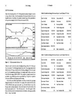
A characteristic of the ADX is that a rising value indicates a strengthening
trend. This is true, but a stock develops a strong trend well before the ADX re-
flects the movement of the stock. Geometric breakouts from a long or short base
trigger signals much earlier. The stock in Figure 1.12 had a 30% move before
the 14-day ADX even reached 30 in late September.
1.4 A Trading Model
31
Each technical indicator has its niche, however. As shown in Figure 1.12, high
ADX readings are useful for pullbacks (denoted by P) in very strong trends. A
retracement of two or more bars is usually interrupted by a resumption of the
prevailing long-term trend.
Returning to the example, a strong reversal begins in early October, and the
ADX does not resume rising until well into the reversal. Thus, treat the ADX as
a lagging indicator-the trader will benefit from shortening the study length
from 14 to 7, especially for short sales.
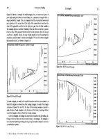
Directional Movement Index (DMI)
The DMI has 2 components: +DMI and -DMI. If +DMI is greater than -DMI,
then the trend is up, and if the -DMI is greater than +DMI, then the trend is
down. Figure 1.13 shows a crossover of the two lines under the 50-day moving
average. Combined with a weakening ADX trend (the thick line), this cross-
over is typically a good shorting opportunity, and the same principle applies to

long positions initiated above the 50-day moving average.
In Figure 1.13, the DMI lines widen near the end of the chart (beginning of
March). When the spread between the two values is wide, a position should be
covered. In this case, the down tick in -DMI corresponding with the up tick in
+DMI is an opportunity to either cover a short position or go long.
32
1 Introduction
1.5 Performance
This section establishes some guidelines on evaluating trading system perform-
ance using the TradeStation Performance Report. For a thorough evaluation of
a trading system, refer to Stridsman's book Trading Systems That Work [30]. As
the trader will discover, the key to any trading system is to analyze its drawdown
in terms of losing streaks and the size of the average losing trade. Based on these
data, we can calculate the appropriate amount of capital to risk per trade.
Table 1.8 shows a sample performance report. The Total Net Profit and
Percent profitable numbers are alluring, but the important number is the Profit
Factor: the number of dollars gained for each one lost. In this example, dividing
the Gross Profit of $447,001.50 by the Gross Loss of $174,787.00 yields a
profit factor of 2.56.
Reviewing some other ratios, the ratio of the average win to the average loss
is $4,217.00 divided by $2,361.99 equals 1.79. The holding period ratio is the
average number of bars in the winners (30) divided by the average number of
bars in the losers (16), approximately 1.88.
Table
1.8.
TradeStation
Strategy
Performance
Report
—

A
System
QQQ-10
min
Total Net Profit
Gross Profit
Total # of trades
Number winning trades
Largest winning trade
Average winning trade
Ratio avg win/avg loss
Max consec. Winners
Avg # bars in winners
Max intraday drawdown
Profit Factor
$272,214.50
$447,001.50
180
106
$12,168.00
$4,217.00
1.79
7
30
($21,993.00)
2.56
Open position P/L
Gross Loss
Percent profitable
$0.00

($174,787.00)
58.89%
Number losing trades 74
Largest losing trade ($5,280.00)
Average losing trade ($2,361.99)
Avg trade (win & loss) $1,512.30
Max consec. losers 5
Avg # bars in losers 16
Max # contracts held 9,500
To assess the impact of drawdown, multiply the largest losing trade ($5,280.00)
by the maximum consecutive losers (5) to get $26,400.00. The actual maximum
drawdown (not shown in the table) was $19,720.00. The maximum intraday
drawdown of $21,993.00 occurred when the system was short before a surprise
interest rate cut, so we are fortunate to have this price shock in the results.
1.5 Performance
33
We look for month-to-month consistency with any trading system, as shown in
Table 1.9. Day traders should expect consistent weekly profitability. A swing
trader should expect occasional losing weeks because the combination of time
frame and losing streak makes it almost impossible to avoid a losing week. For
example, if the trader makes five trades a week and the maximum consecutive
losers is four, then the odds of a losing week are highly probable. Compare the
actual monthly performance with the expected monthly income in Table 1.3 to
set reasonable profit goals.
Table 1.9. Monthly Analysis
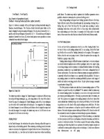
As displayed in Figure 1.14, the Equity Curve (EC) is a graph of the cumulative
profit of a set of trading systems. The vertical distance between each point on
the chart represents the profit or loss of an individual trade. The EC is just like a
price chart-it has trend and it has pullbacks (the distance from peak to trough is
the drawdown). Technical indicators such as the moving average and ADX can

be calculated for the curve to assess the strength of a trading system.
Analyze the Equity Curve from a three-month perspective because a trader
should expect flat periods lasting up to thirty or sixty days for a system. The EC
in Figure 1.14 has roughly the same net profit for each three-month period. Plot
the EC every month to determine whether or not the system performance is
deteriorating, e.g., , it advances half as much over consecutive periods.