foucault and kadan-limit order book as a market for liquidity
Bạn đang xem bản rút gọn của tài liệu. Xem và tải ngay bản đầy đủ của tài liệu tại đây (460.1 KB, 59 trang )
Limit Order Book as a Market for
Liquidity
1
Thierry Foucault
HEC School of Management
1 rue de la Liberation
78351 Jouy en Josas, France
Tel: 33-1-39679411
Ohad Kadan
School of Business Administration
Hebrew University,
Jerusalem, 91905, Israel
Tel: 972-2-5883232
Eugene Kandel
School of Business Administration
and Department of Economics
Hebrew University,
Jerusalem, 91905, Israel
Tel: 972-2-5883137
July 10, 2001
1
We would like to thank David Easley, Frank de Jong, Larry Glosten, Larry Harris,
Pete Kyle, Leslie Marx, Narayan Naik, Maureen O'Hara, Christine Parlour, Patrik Sandas,
Ilya Strebulaev, Avi Wohl, and seminar participants at Amsterdam, Emory, Illinois, Insead,
Jerusalem, LBS, Tel Aviv, Wharton for their helpful comments and suggestions. Comments
by participants at the WFA2001 meeting and the Gerzensee Symposium2001 have been
helpful as well. The authors thank J. Nachmias Fund, and Kruger Foundation for ¯nancial
support.
Abstract
We develop a dynamic model of an order-driven market populated by discretionary
liquidity traders. These traders must trade, yet can choose the type of order and
are fully strategic in their decision. Traders di®er by their impatience: less patient
traders demand liquidity, more patient traders provide it. Three equilibrium types
are obtained - the type is determined by three parameters: the degree of impatience
of the patient traders, which we interpret as the cost of execution delay in providing
liquidity; their proportion in the population, which determines the degree of com-
petition among the liquidity providers; and the tick size, which is the cost of the
minimal price improvement. Despite its simplicity, the model generates a rich set of
empirical predictions on the relation between market parameters, time to execution,
and spreads. We argue that the economic intuition of this model is robust, thus its
main results will remain in more general models.
1 Introduction
Limit and market orders constitute the core of any order-driven continuous trading
system (such as the NYSE, London Stock Exchange, Euronext, Tokyo and Toronto
Stock Exchanges, as well as all the ECNs).
1
A market order guarantees an immedi-
ate execution at the best price available at the moment of the order arrival at the
exchange. In general, a market order represents demand for liquidity (immediacy of
execution). With a limit order, a trader can improve his execution price relative to
the market order price, but the execution is neither immediate, nor certain. A limit
order represents supply of liquidity to future traders.
2
The optimal order choice ultimately involves a tradeo® between the cost of a
delayed execution and the cost of immediate execution, which (for small transactions)
is determined by the size of the inside spread. Intuitively we expect patient traders
to post limit orders and supply liquidity to impatient traders, who opt for market
orders. In his seminal paper Demsetz (1968) stresses the limit orders as the source of
liquidity, pointing out the trade o® between longer execution time and better prices.
He states (p.41):
\Waiting costs are relatively important for trading in organized markets, and would
seem to dominate the determination of spreads."
He conjectures that more aggressive limit orders will be submitted to gain priority
in execution and shorten the expected time-to-execution. Moreover, he anticipates
that the active securities should have lower spreads because the competition from
limit orders will be ¯ercer in light of shorter waiting times. In this paper we explore
the interactions between traders' impatience, order placements strategies and waiting
times in the context of a dynamic order-driven market.
Our model features buyers and sellers arriving sequentially. Each trader wants
1
Domowitz (1993) shows that over 30 important ¯nancial markets in the world in the early 90's
had some of order-driven market features in their design. The importance of order-driven markets
around the world has been steadily increasing since.
2
We ignore here marketable limit orders.
1
to buy or sell one unit of a security. We assume that these are liquidity traders,
i.e. they will buy/sell regardless of price. However, they choose between market and
limit orders so as to minimize their cost of trading. Upon arrival, the traders decide
to place a market order or a limit order, conditional on the state of the book. If
submitting a limit order the trader chooses a price and bears the opportunity cost of
postponing the trade.
Under several simplifying assumptions we are able to develop a recursive method
for calculating the order placements strategies and the expected time-to-execution for
limit orders. In general, in equilibrium, patient traders provide liquidity to impatient
traders. We identify 3 types of equilibria characterized by markedly di®erent dynamics
for the limit order book. These dynamics turn out to be very sensitive to the ratio
of the proportion of patient traders to the proportion of impatient traders. Actually
the larger is this ratio, the more intense is competition among liquidity suppliers.
They are also in°uenced by the dispersion of waiting costs across traders. Some of
our main ¯ndings can be summarized as follows.
² Limit orders time-to-execution are large when the proportion of patient traders
is relatively large. This e®ect enhances competition among liquidity providers
who submit more aggressive orders to shorten their time-to-execution. Hence
markets with a relatively large proportion of patient traders feature smaller
spreads.
² In order to speed up execution, traders frequently ¯nd optimal to undercut
or outbid the best quotes by more than one tick. This happens when (i) the
proportion of patient traders is relatively large, (ii) waiting costs are large or
(iii) the tick size is small.
² A decrease in the tick size can result in larger expected spreads. Actually it
gives the possibility to traders to quote less competitive prices by expanding
2
the set of prices. If competition among liquidity providers is weak, they use the
new prices and the average spread increases.
² A decrease in the order arrival rate can result in smaller expected spreads.
Intuitively, such a decrease extends the expected time-to-execution for limit
orders. This e®ect induces liquidity suppliers to place more aggressively priced
limit orders when the inside spread is large.
In some limit order markets, designated market-makers are required to enter bid
and ask quotes in the limit order book. This is the case, for instance, in the Paris
Bourse for medium and small capitalization stocks.
3
We consider the e®ect of intro-
ducing this type of trader in our model. We show that the presence of a trader who
monitors the market and occasionally submits limit orders, can signi¯cantly alter the
equilibrium. His intervention forces patient traders to submit more aggressive o®ers
in order to speed up execution and hence narrows the spreads. This result provides
important guidance for market design.
Our results contribute to the growing literature on limit order markets. Most of
the models in the theoretical literature are focused on the optimal bidding strategies
for limit order traders (see e.g. Glosten (1994), Chakravarty and Holden (1995),
Rock (1996), Seppi (1997), Biais, Martimort and Rochet (2000), Parlour and Seppi
(2001)). These models do not analyze the choice between market and limit orders and
are static. For this reason they do not describe the interactions between impatience,
time-to-execution and order placement strategies as we do in this paper.
Parlour (1998) and Foucault (1999) study dynamic models. Parlour (1998) shows
how the order placement decision is in°uenced by the depth available at the inside
quotes. Foucault (1999) analyzes the impact of the risk of being picked o® and the
risk of non execution on traders' order placement strategies. In both models, limit
order traders do not bear waiting cost. Hence time-to-execution does not in°uence
3
In the Paris Bourse, the designated market-makers are required to post bid-and ask quotes for
a minimum number of shares and their spread cannot exceed 5% of the stock price.
3
traders' bidding strategies in these models whereas it plays a central role in the present
article.
4
We are not aware of other theoretical papers in which prices and time-to-execution
for limit orders are jointly determined in equilibrium. Time-to-execution, however,
is an important dimension of market quality in limit order markets (see SEC 1997).
Lo, McKinlay and Zhang (2001) estimate various econometric models for the time-to-
execution of limit orders. Some of their ¯ndings are consistent with our results, e.g.
the expected time-to-execution increases with the distance between the limit price
and the mid-quote. Our model also generates new predictions that could be tested
with data on actual time-to-execution for limit orders. For instance we show that the
average time-to-execution (across all limit orders) depends on (i) the tick size, (ii)
the order arrival rate and (iii) the proportion of patient traders.
5
Biais, Hillion and
Spatt (1995) describe the interactions between the size of the inside spread and the
order °ow.
6
They observe that limit order traders quickly improve the inside spread
when it is large. In our model the amount by which a limit order trader undercuts or
outbids the best o®ers depends on (i) the inside spread, (ii) the proportion of patient
traders and (iii) the order arrival rate. These ¯ndings provide guidance for empirical
studies of limit order markets.
7
The paper is organized as follows. Section 2 describes the model. Section 3
derives the equilibrium of the limit order market and provides examples. In Section
4
A few authors suggest other approaches to modeling the limit order book. This includes Angel
(1994), Domowitz and Wang (1994) and Harris (1995) who consider models with exogenous order
°ow. Using queuing theory, Domowitz and Wang (1994) analyze the stochastic properties of the
book. Angel (1994) and Harris (1995) study how the optimal choice between market and limit
orders varies according to di®erent market conditions (e.g. the state of the book, the rate of order
arrival ). We use more restrictive assumptions than these authors. But these assumptions enable
us to endogenize the order °ow and the time-to-execution for limit orders.
5
Lo et al. (2001) report that there is a large variation in mean time-to-execution across stocks.
According to our model, these variations can be explained by the fact that stocks di®er with respect
to trading activity or tick size.
6
See also Benston, Irvine and Kandel (2001).
7
Empirical analyses of limit order markets include Goldstein and Kavajecz (2000), Handa and
Schwartz (1996), Harris and Hasbrouck (1996), Holli¯eld, Miller and Sandas (2001a,b), Kavajecz
(1999) and Sandas (2000).
4
4 we explore the e®ect of a change in tick size and a change in traders' arrival rate on
measures of market quality. Section 5 presents some extensions. Section 6 concludes.
All proofs (except for Proposition 1) are in the Appendix.
2 Model
2.1 Timing and Market Structure
Consider a continuous market for a single security, organized as a limit order book
without intermediaries. We assume that latent information about the security value
determines the range of admissible prices, however the transaction price itself is de-
termined by traders who submit market and limit orders.
8
Speci¯cally, at price A
outside investors stand ready to sell an unlimited amount of security, thus the sup-
ply at A is in¯nitely elastic. We also assume that there exists an in¯nite demand
for shares at price B (B < A). Moreover, A and B are constant over time. These
assumptions assure that all the prices in the limit order book are in the range [B; A].
9
The goal of this model is to investigate the behavior of the limit order book and
transaction prices within this interval. This behavior is determined by the supply
and demand of liquidity, or in other words by optimal submission of market and limit
orders.
This is an in¯nite horizon model with discrete time periods. At the beginning
of every period a trader arrives at the market and observes the limit order book.
Each trader must buy or sell one unit of the security. These liquidity traders have a
discretion on which type of order to submit. Each trader can submit a market order
to ensure an immediate trade at the best quote available at the time. Alternatively,
he can submit a limit order, which improves the price, but delays the execution. We
assume that traders' waiting costs are proportional to the time they have to wait until
8
We discuss this modelling strategy below.
9
A similar assumption is used in Seppi (1997) and Parlour and Seppi (2001).
5
completion of their transaction. Hence traders face a trade-o® between the execution
price and the time-to-execution when they choose between market and limit orders.
In contrast with Admati and P°eiderer (1988) or Parlour (1998), traders are not
required to carry their desired transaction by a deadline.
All prices (but not waiting costs and traders' valuations) are placed on a discrete
grid. The tick size, which is chosen by the exchange designer, is denoted by ¢ > 0.
All the prices in the model are expressed in terms of integer multiples of ¢. We
denote by a and b the best ask and bid quotes when a trader comes to the market.
The inside spread at that time is s := a ¡ b. Given the setup we know that a · A,
b ¸ B, and s · K := A ¡ B.
10
Both buyers and sellers can be of two types which di®er by the size of their
waiting costs. Type 1 traders (the patient type) incur an opportunity cost of d
1
for
an execution delay of one period. Type 2 traders (the impatient type) incur a cost
of d
2
(0 · d
1
< d
2
). The proportion of patient traders in the population is denoted
by µ (0 < µ < 1). Patient types can be thought as institutions building up positions,
or other long-term investors. Arbitragers or brokers conducting agency trades are
examples of impatient traders.
Limit orders are stored in the limit order book and are executed in sequence
according to price priority (e.g. sell orders with the lowest o®er are executed ¯rst).
For tractability, we make the following simplifying assumptions about the market
structure.
A.1: Each trader arrives only once, submits a market or a limit order and exits.
Submitted orders cannot be cancelled or modi¯ed.
A.2: Traders who submit limit orders must narrow the spread by at least one
tick.
10
Notice that a; b; s;A; B;K and all other spreads and prices that follow are positive integers. This
is so since we use integer multiples of the tick size, ¢; instead of dollar prices and dollar spreads.
Furthermore the model does not require time subscripts on variables, thus they are omitted for
brevity.
6
A.3: Buyers and sellers alternate with certainty, e.g. ¯rst a buyer arrives, then a
seller, then a buyer, and so on. The ¯rst trader is a buyer with probability 0.5.
Assumption A.1 implies that traders in the model do not adopt active trading
strategies which may involve repeated submissions and cancellations. These active
strategies require market monitoring, which is costly (e.g. because liquidity traders'
time is valuable). The second assumption implies that limit order traders cannot
queue at the same price (note however that they queue at di®erent prices since limit
orders do not drop out of the book). With this assumption, the inside spread is
the only state variable which in°uences traders' order placement strategies. This
greatly simpli¯es the description and the characterization of traders' order placement
strategies. This assumption is less restrictive than it may appear. In Section 6, we
show that we can dispense with assumption A2 if patient traders' waiting cost is
large enough. The third assumption facilitates the computation of traders' expected
waiting time and is imperative to keep the model tractable (see Section 3.1. for a
discussion).
Let p
b
and p
s
be the prices paid by buyers and sellers, respectively. In our model,
as in Admati and P°eiderer (1988) for instance, traders do not have the option not
to trade. Thus their only decision is a choice of strategy resulting in a trade. A
buyer can either pay the lowest ask a or submit a limit order which creates a new
inside spread with size j. In a similar way, a seller can either receive the largest bid
b or submit a limit order which creates a new inside spread with size j. This choice
determines the execution price:
p
b
= a ¡ j; p
s
= b + j with j 2 f0; :::; s ¡ 1g;
where j = 0 represents a market order. It is convenient to consider j (rather than
p
b
or p
s
) as the trader's decision variable. For brevity, we say that a trader uses a
\j-limit order" when he posts a limit order which creates a spread with size j. The
expected time-to-execution of a j-limit order is denoted by T(j). Since the waiting
7
costs are assumed to be linear in waiting time, the expected waiting cost of a j-limit
order is d
i
T(j), i 2 f1; 2g: As a market order entails immediate execution, we set
T(0) = 0.
We assume that traders are risk neutral. The expected pro¯t of trader i (i 2 f1; 2g)
who submits a j-limit order is:
¦
i
(j) =
8
>
<
>
:
V
b
¡ p
b
¢ ¡ d
i
T(j) = (V
b
¡ a¢) + j¢ ¡ d
i
T (j) if trader i is a buyer
p
s
¢ ¡ V
s
¡ d
i
T (j) = (b¢ ¡ V
s
) + j¢ ¡ d
i
T (j) if trader i is a seller
where V
b
, V
s
are buyers' and sellers' valuations, respectively. To justify this classi¯ca-
tion to buyers and sellers, we assume that V
b
>> A¢, and V
s
<< B¢.
11
Expressions
in parenthesis represent pro¯ts associated with market order submission. These prof-
its are determined by the trader's valuation and the best quotes when he submits
his market order. It is immediate that the optimal order placement strategy when
the inside spread has size s solves the following optimization problem, for buyers and
sellers alike:
max
j2f0;:::s¡1g
¼
i
(j) := j¢ ¡ d
i
T(j): (1)
We will show that T(j) is non-decreasing in j, in equilibrium. Hence a better
execution price (larger value of j) is obtained at the cost of a larger expected waiting
time.
A strategy for a trader is a mapping that assigns a j-limit order, j 2 f0; :::; s ¡1g;
to every possible spread s 2 f1; :::; Kg. Thus, a strategy determines which order to
submit given the size of the inside spread. At the beginning of the game we set:
a = A and b = B hence s = K: Let o
i
(:) be the order placement strategy of a
trader with type i. A trader's optimal strategy depends on future traders' actions
since they determine his expected waiting time, T (¢): Consequently a subgame perfect
equilibrium of the trading game is a pair of strategies, o
¤
1
(:) and o
¤
2
(:), such that the
order prescribed by each strategy for every possible inside spread solves Program (1)
11
Traders' valuations for the security can consist of common and idiosyncratic components as in
Foucault (1999) or Holli¯eld, Sandas and Miller (2001a,b).
8
when the expected waiting time T(¢) is computed using the fact that traders follow
strategies o
¤
1
(:) and o
¤
2
(:).
12
2.2 Discussion
It is worth stressing that we abstract from the e®ects of asymmetric information and
information aggregation. This is a marked departure from the \canonical model"
in theoretical microstructure literature, surveyed in Madhavan (2000), and requires
some motivation.
In most market microstructure models, quotes are determined by agents who
have no reason to trade, and either trade for speculative reasons, or make money
providing liquidity. For these value-motivated traders, the risk of trading with a
better informed agent is a concern and a®ects the optimal order placement strategies.
In contrast, in our model, traders have a non-information motive for trading and
are precommited to trade. The risk of adverse selection is not an issue for these
liquidity traders. Rather, they determine their order placement strategy with a view
at minimizing their transaction cost and balance the cost of waiting against the cost
of obtaining immediacy in execution.
13
In order to focus on this trade-o® in the
simplest way, we propose a framework that allows for a simple dichotomy between
\macro" information-based asset pricing and market \micro"structure. We assume
that information-related considerations determine the price range, rather than the
price itself. The equilibrium in the market for liquidity provision determines quotes
inside this range. At this stage we do not model the determination of this range, but
rather assume that it exists. For ¯xed income securities these boundaries are quite
natural, given the existence of close substitutes. In case of equities we conjecture
that this price range represents the consensus among all analysts/investors, yet is not
12
The rules of the game, as well as all the parameters are assumed to be common knowledge
among all the traders.
13
Harris (1998) and Glosten (2000) also argue that optimal order placement strategies are di®erent
for liquidity traders and value-motivated traders.
9
subject to arbitrage (see Shleifer and Vishny 1997).
The trade-o® between the cost of immediate execution and the cost of delayed
execution may be relevant for value-motivated traders as well. However, it is very
di±cult to solve dynamic models with asymmetric information among traders who
can strategically choose between market and limit orders. In fact we are not aware
of such dynamic models.
14
3 Equilibrium Patterns
In this section we characterize the equilibrium strategies for each type of trader. For
given values of the parameters, the equilibrium is unique. We also calculate the
stationary probability distribution of the inside spread in equilibrium. The dynamics
of the order °ow and the distribution of the inside spread depend on (i) the proportion
of patient traders relative to the proportion of impatient traders and (ii) the di®erence
in waiting costs between patient and impatient traders. This leads us to distinguish
between three di®erent types of equilibria. We provide examples which illustrate the
attributes of each one of the three equilibrium types.
3.1 Expected Waiting Time
In order to characterize the equilibrium, we ¯rst analyze the behavior of the expected
waiting time function T (j). Suppose the trader arriving this period chooses a j-limit
order. We denote by ®
k
(j) the probability that the trader arriving next period and
observing an inside spread with size j chooses a k-limit order, k 2 f0; 1; :::; j ¡ 1g.
15
Clearly ®
k
(j) depends on traders' strategies and
j¡1
X
k=0
®
k
(j) = 1; 8j = 1; :::; K ¡ 1:
14
Chakravarty and Holden (1995) consider a single period model in which informed traders can
choose between a market and a limit orders. Glosten (1994) or Biais et al.(2000) consider limit order
markets with asymmetric information but do not allow traders to choose between market and limit
orders.
15
Recall that k = 0 stands for a market order.
10
Assumption A.2 implies that a trader who faces a one tick spread submits a market
order. Consequently, the time-to-execution for a 1-limit order is one period, i.e.
T(1) = 1. Next, we establish a general recursive formula for the expected waiting
time function. This formula links the expected waiting time function to traders' order
placement strategies (described by the ®s
0
).
Lemma 1 If ®
0
(j) > 0; the expected waiting time for the execution of a j-limit order
is given by the following recursive formula:
T(j) =
1
®
0
(j)
2
4
1 +
j¡1
X
k=1
®
k
(j)T (k)
3
5
8j = 2; :::; K ¡ 1 and T(1) = 1 (2)
Two extreme cases are worth emphasizing. The ¯rst is when no trader submits
a market order when he faces a spread with size j
¤
. In this case ®
0
(j
¤
) = 0 and the
expected waiting time of a j-limit order, with j ¸ j
¤
, is in¯nite. Such limit orders
will never be submitted in equilibrium, since they are dominated by a market order.
Hence, in equilibrium, the expected waiting time of limit orders is always ¯nite. This
implies that limit orders execute with certainty.
16
The second case is when all traders
submit a market order when they face a spread with size j
¤¤
. In this case T(j
¤¤
) = 1.
It will become apparent that no spreads smaller than j
¤¤
and larger than j
¤
can be
observed in equilibrium. In between, there is a variety of cases in which some traders
¯nd it optimal to submit limit orders, while others submit market orders.
Assumption A.3 is used to obtain the expected waiting function (Eq.(2)). The
alternation of buyers and sellers yields a simple ordering of the queue of un¯lled
limit orders (the book): a j-limit order cannot be executed before j
0
-limit orders
where j
0
< j: This is of course true when we consider two buy or two sell limit orders
because of price priority. Without A.3, this would not be true however if the j-limit
order and the j
0
-limit order are in opposite direction (a buy order and a sell order
for instance). The ordering implied by A.3 explains why the expected waiting time
16
However, execution may take place after a very long time. In fact, in any ¯nite time interval,
the execution probability of a j-limit order is strictly smaller than 1; if T(j) > 1.
11
has a simple recursive structure. Without this recursive structure, it becomes very
di±cult to compute the expected waiting time function and the model is (in general)
intractable.
3.2 Equilibrium strategies
Although the trading game has an in¯nite horizon, the nodes with one-tick spread
serve as end-nodes in the usual ¯nite game trees, since everybody submit a market
order. Thus we can solve the game by backward induction. To see this point, consider
a trader who arrives in the market when the size of the inside spread is s = 2: The
trader has two choices: either he submits a market order or a 1-limit order. The latter
improves his execution price by one tick compared to a market order but results in a
one period delay in execution. Choosing the best action for each type of trader, we
determine ®
k
(2) (for k = 0 and k = 1). If ®
0
(2) = 0, the expected waiting time for a
2-limit order is in¯nite. It follows that no spread larger than one tick can be observed
in equilibrium. If ®
0
(2) > 0;we compute T(2) (using Eq.(2)). Then we proceed to
s = 3 and so forth. This inductive approach is the key to most results in the paper.
Three results follow immediately. First, as this is a game of perfect information an
equilibrium in pure strategies always exists. Second, since this is a one-play game for
each trader, there are no Nash equilibria (in pure strategies) other than the sub-game
perfect equilibria that we trace by backward induction. And third, the equilibrium is
unique for any tie-breaking rule. We choose the following rule. If a trader is indi®erent
between a j
1
-limit order and a j
2
-limit order, with j
1
< j
2
, he submits the limit order
with the smallest spread (in this case the j
1
-limit order).
We proceed by proving results that characterize the equilibrium. Traders submit
limit orders only if they can cover their waiting cost. Since limit orders wait at least
one period, there is a spread below which a trader strictly prefers to use market orders.
We refer to this spread as being the trader's \reservation spread" and we denote it j
R
i
for trader i (i 2 f1; 2g). This the smallest spread trader i is willing to establish with
12
a limit order, and still the associated expected pro¯t is greater than zero (dominates
a market order). In order to give a formal de¯nition of the reservation spread, let
int(x) be the largest integer smaller than or equal to x. The reservation spread of
trader i is:
17
j
R
i
:= int(
d
i
¢
) + 1 i 2 f1; 2g (3)
Clearly, the reservation spread of a patient trader cannot exceed that of an impatient
one, however the two can be equal. The latter case yields the ¯rst equilibrium type for
all values of other parameters. We say that the two trader types are indistinguishable
if they possess the same reservation spreads: j
R
:= j
R
1
= j
R
2
. Intuitively, traders
are indistinguishable if the two waiting costs fall into the same cell on the grid:
[0; ¢); [¢; 2¢); [2¢; 3¢); :::.
Proposition 1 Suppose traders' types are indistinguishable (j
R
1
= j
R
2
= j
R
) then, in
equilibrium all traders submit a market order if s · j
R
and submit a j
R
-limit order
if s > j
R
.
The proof of Proposition 1 is simple and intuitive hence we present it here instead
of relegating it to the Appendix. Consider a trader who arrives in the market when
the inside spread is s > j
R
. If he submits a j-limit order with j
R
< j then the next
trader submits a j
R
-limit order given the speci¯cation of traders' strategies. This
implies that ®
0
(j) = 0 (i.e. the waiting time is in¯nite) for j
R
< j: Therefore a
j-limit order with j
R
< j cannot be optimal since it is never executed. If the trader
submits a j
R
-limit order; his order is cleared by the next trader. By de¯nition of the
reservation spread, this choice dominates a market order. This establishes that when
the inside spread is larger than traders' reservation price, the optimal strategy is to
submit a j
R
-limit order. Finally consider a trader who arrives in the market when the
spread is s · j
R
. By de¯nition of the reservation spread, the submission of a market
17
A trader who submits a limit order waits a least one period before execution. Hence the smallest
waiting cost for a trader with type i is d
i
: It follows that the smallest spread trader i can establish
is the smallest integer, j
R
i
; such that ¼
i
(j
R
i
) = j
R
i
¢ ¡ d
i
> 0. This remark yields Eq.(3).
13
order is a dominant strategy for this trader. This completes the proof of Proposition
1.
The equilibrium with indistinguishable traders is characterized by an oscillating
pattern. The ¯rst, as well as every odd-numbered trader afterwards, submits a limit
order which creates a spread with size j
R
. The second, and every even-numbered
trader afterwards, submits a market order. The inside spread oscillates between K
and j
R
and transactions take place only when the spread is small. Trade prices are
either A ¡ j
R
if the ¯rst trader is a buyer, or B + j
R
, if the ¯rst buyer is a seller.
The outcome is competitive in the sense that limit order traders always quote their
reservation spread, that is the spread such that they just cover their waiting cost.
18
After characterizing the ¯rst type of equilibrium, we proceed by assuming that
traders are heterogeneous: j
R
1
< j
R
2
. Given two spreads j
1
< j
2
we denote by hj
1
; j
2
i
the set: fj
1
; j
1
+ 1; j
1
+ 2; :::; j
2
g, i.e. the set of all possible spreads between j
1
and j
2
(inclusive). In particular, the range of all possible spreads is h1; Ki.
Proposition 2 Suppose traders are heterogeneous (j
R
1
< j
R
2
). In equilibrium there
exists a cuto® spread s
c
2 hj
R
2
; Ki such that:
1. Given a spread s 2 h1; j
R
1
i; patient and impatient traders submit a market order.
2. Given a spread s 2 hj
R
1
+ 1; s
c
i; a patient trader submits a limit order and an
impatient trader submits a market order.
3. Given a spread s 2 hs
c
+ 1; Ki; patient and impatient traders submit a limit
order.
The proposition shows that when j
R
1
< j
R
2
, the state variable s (the inside spread)
is partitioned into three regions: (i) s · j
R
1
, (ii) j
R
1
< s · s
c
and (iii) s > s
c
: The
18
Observe that the tick size determines the resolution of traders' categories. The larger is the tick
size - the more traders with di®ering waiting costs are pooled together into the same equilibrium
strategies. Conversely observe that d
1
and d
2
may be arbitrarily close and still fall into di®erent
cells of the grid if the tick size is su±ciently small.
14
reservation spread of the patient trader, j
R
1
, represents the smallest spread observed
in the market. At the other end s
c
is the largest quoted spread in the market. Limit
orders which create a larger spread have an in¯nite waiting time since no traders
submit a market order when the inside spread is larger than s
c
. Hence these limit
orders are never submitted. This observation permits us to restrict our attention to
cases where s
c
= K; for brevity. This equality holds true when the cost of waiting for
an impatient trader is su±ciently large.
19
Under this condition impatient traders al-
ways demand liquidity (submit market orders), while patient traders supply liquidity
(submit limit orders) when the inside spread is larger than their reservation spread.
Proposition 3 Suppose s
c
= K: Any equilibrium exhibits the following structure:
there exist q spreads, n
1
< n
2
< ::: < n
q
, with n
1
= j
R
1
, n
q
= K and 2 · q · K; such
that the optimal order submission strategy is as follows:
² An impatient trader submits a market order, for any spread in h1; Ki.
² A patient trader submits a market order when he faces a spread in h1; n
1
i and
submits a n
h
-limit order when he faces a spread in hn
h
+ 1; n
h+1
i for h =
1; :::; q ¡ 1.
Hence when a patient trader faces an inside spread with size n
h+1
> j
R
1
; he
responds by submitting a limit order which improves upon the inside spread by
(n
h+1
¡ n
h
) ticks. This order establishes a new inside spread equal to n
h
. When
the inside spread is K; it takes a streak of q ¡ 1 patient traders to bring the inside
spread to the competitive level j
R
1
: Hence q determines the maximal number of limit
orders which can be observed in the book. We refer to q as the length of the book: A
small length of the book means that patient traders quickly make good o®ers since it
takes a few patient traders to bring the spread to the competitive level.
19
For instance, s
c
= K if j
R
2
¸ K: It is worth stressing that this condition is su±cient but not
necessary. In Examples 2 and 3 below, j
R
2
is much smaller than K but s
c
= K:
15
Next we analyze the expected waiting time in equilibrium. Let r :=
µ
1¡µ
be the
ratio of the proportion of patient traders to the proportion of impatient traders.
Intuitively, when this ratio is smaller (larger) than 1, liquidity is consumed more
(less) quickly than it is supplied. As we show below, this ratio determines traders'
bidding strategies and time-to-execution for limit orders.
Proposition 4 The expected waiting time function in equilibrium is given by:
T (n
1
) = 1 and T(n
h
) = 1 + 2
h
X
k=2
r
k¡1
for h = 2; :::; q ¡ 1;
and
T(j) = T(n
h
) 8 j 2 hn
h¡1
+ 1; n
h
i:
Clearly the expected waiting time function (weakly) increases with j. Hence the
larger is the distance between the price of a limit order and the mid-quote, the larger
is the expected waiting time for the order. This result is consistent with the evidence
in Lo, McKinley and Zhang (2001).
Another determinant of the expected waiting time is the proportion of patient
traders relative to the proportion of impatient traders, r. The intuition is as follows.
Notice that h determines the priority status of a limit order in the queue of un¯lled
limit orders. Actually an n
h
-limit order can not be executed before n
h
0
-limit orders
have been executed if h
0
< h (when these orders are present in the book, of course).
When r increases, the likelihood of a market order decreases. It follows that the
expected waiting time for the h
th
limit order in the queue enlarges. It turns out that
the rate of increase in the waiting time from one limit order to the next in the queue of
limit orders depends on r as well. Actually when r > 1(r < 1) the marginal expected
waiting time T (n
h
) ¡ T(n
h¡1
) is non-decreasing (non-increasing) in h. In this case,
we say that T(¢) is \convex" (\concave") in h. The next corollary summarizes these
remarks.
16
Corollary 1 The expected waiting time of the h
th
limit order in the queue of limit
orders increases with r, the ratio of the proportion of patient traders to the proportion
of impatient traders. The expected waiting time function is \convex" when r > 1; and
\concave" when r < 1 .
We show below that these properties of the expected waiting time function in°u-
ence traders' bidding strategies. In the next proposition we express the spreads on
the equilibrium path, i.e. n
1
; n
2
; ::;n
q
, in terms of the exogenous parameters. De-
¯ne ª
h
:= n
h
¡ n
h¡1
for h ¸ 2 as the spread improvement, when the inside spread
has a size equal to n
h
. The spread improvement is the number of ticks by which a
trader narrows the spread when he submits a limit order. The larger is the spread
improvement, the more aggressive is the limit order.
Proposition 5 The set of equilibrium spreads is given by:
n
1
= j
R
1
; n
q
= K;
n
h
= n
1
+
h
X
k=2
ª
k
h = 2; :::; q ¡ 1;
where
ª
h
= int(2r
h¡1
d
1
¢
) + 1
and the length of the book, q is the smallest integer such that:
j
R
1
+
q
X
k=2
ª
k
¸ K: (4)
The previous proposition shows that whenever, 2d
1
r
h¡1
¸ ¢, a limit order trader
¯nds optimal to undercut or to outbid the best prices by more than one tick (ª
h
> 1).
Biais, Hillion and Spatt (1995) observe that liquidity suppliers frequently improve
upon the best quotes by several ticks. Our result identi¯es four determinants for
the spread improvement which could be considered in future empirical investigation.
17
These determinants are: (i) the proportion of patient traders, r, (ii) the per period
waiting cost, d
1
(iii) the tick size, ¢, and (iv) the inside spread. We analyze each of
these determinants in turn.
When r increases, the time-to-execution for a given position in the queue of limit
orders becomes larger. Hence, other things equal, liquidity suppliers bear larger wait-
ing costs (d
1
T): Traders react by submitting more agressive orders to preempt good
positions in the queue of limit orders and thereby reduce their time-to-execution. The
same e®ect operates when d
1
increases. In this case, traders bear larger waiting costs
because the per-period waiting cost is larger. The smaller is the tick size, the smaller
is the cost of improving upon the best bid and ask prices. Thus a smaller tick results
in larger spread improvements in terms of ticks.
The spread improvement, ª
h
, increases (decreases) with h when r > 1 (r < 1):
This means that when r > 1 the spread improvement increases with the size of the
inside spread, while the opposite is true when r < 1. The intuition is as follows.
Consider the (h ¡1)
th
trader in the queue of un¯lled limit orders . This trader's time
to execution is T(n
h¡1
) instead of T (n
h
) for the trader behind him in the queue. Hence
the di®erence in expected waiting cost between the h
th
and the (h ¡ 1)
th
positions in
the queue of limit orders is equal to (T(n
h
) ¡ T(n
h¡1
))d
1
. Intuitively, this should be
the \price" of acquiring the (h ¡1)
th
position instead of the h
th
position in the queue.
The dollar spread improvement plays the role of this price and, for this reason, it
is approximately equal to (T(n
h
) ¡ T(n
h¡1
))d
1
:
20
This shows that the shape of the
waiting time function determines the relationship between the spread improvement
and the inside spread. When r > 1, the waiting time function is convex in h. Hence
liquidity suppliers o®er larger spread improvements when the spread is large. When
r < 1, the waiting time function is concave and liquidity suppliers o®er larger spread
improvements when the spread is small.
20
In fact observe that ª
h
¢ ' 2r
h¡1
d
1
= (T(n
h
) ¡ T(n
h¡1
))d
1
: The dollar spread improvement is
only approximately equal to the di®erence in waiting cost because the set of prices is discrete.
18
Notice that when spread improvements are larger than 1 tick, the traders do not
make use of all the possible prices in equilibrium. This implies that the limit order
book features \holes", i.e. cases in which the distance between two consecutive ask
or bid prices is larger than one tick.
21
The last part of the previous proposition (Eq.(4)) implies that that the length
of the book decreases when spread improvements get larger. Actually, limit order
traders improve on the best quotes by a larger number of ticks so that a smaller
number of prices on the grid are used. This means that more competitive outcomes
are expected when the length of the book is small. This is the case in particular when
r ¸ 1 because (a) spread improvements are large and (b) liquidity is not consumed too
quickly (which leaves time for the inside spread to narrow). For this reason we call the
equilibrium when r ¸ 1 a High Competition (HC) Equilibrium and the equilibrium
when r < 1; a Low Competition (LC) Equilibrium. Using this terminology, we classify
all equilibria in three categories described in Table 1.
Table 1 - Three equilibrium patterns
Equilibrium pattern Description Speci¯cation
Oscillating Indistinguishable Traders j
R
1
= j
R
2
; 8r
Spreads oscillate between K and j
R
:
HC Heterogeneous traders j
R
1
< j
R
2
; r ¸ 1
High level of competition
among liquidity providers
\Convex" time function
LC Heterogeneous traders
Low level of competition j
R
1
< j
R
2
; r < 1
among liquidity providers
\Concave" time function
In the next sections, we show that (i) the stationary probability distribution of
spreads and (ii) the impact of a change in the tick size are strikingly di®erent in HC
and LC equilibria.
21
Holes in the limit order book is a phenomenon documented by several empirical studies: Bi-
ais, Hillion and Spatt (1995) - Paris Bourse; Goldstein and Kavajecz (2000) - NYSE; Holli¯eld,
Miller, and Sandas (2001a) - Stockholm; Benston, Irvine, and Kandel (2001) - Toronto; and Kandel,
Lauterbach, and Tkach (2000) - Tel Aviv.
19
3.3 Examples
We illustrate the three equilibrium patterns by numerical examples. The tick size is
¢ = $0:125. The lower price bound of the book is set to B¢ = $20, and the upper
bound is set to A¢ = $22:5. Thus, the maximal spread is K = 20 (K¢ = $2:5). The
parameters that di®er across the examples are presented in Table 2.
Table 2: Three Examples
Example 1 Example 2 Example 3
(Oscillating) (HC) (LC)
d
1
0:15 0:10 0:10
d
2
0:20 0:25 0:25
µ Any value 0:55 0:45
Table 3 presents the equilibrium strategy for patient (type 1) and impatient (type
2) traders in each example. Each entry in the table presents the optimal limit order
(in terms of ticks) given the current spread (0 stands for a market order).
22
Table 3 - Equilibrium strategies
22
The equilibrium strategies in Examples 2 and 3 follow from the formulae given in Proposition
5.
20
Current Example 1 Example 2 Example 3
Spread Type 1 Type 2 Type 1 Type 2 Type 1 Type 2
1 0 0 0 0 0 0
2 0 0 1 0 1 0
3 2 2 1 0 1 0
4 2 2 3 0 3 0
5 2 2 3 0 3 0
6 2 2 3 0 5 0
7 2 2 6 0 6 0
8 2 2 6 0 7 0
9 2 2 6 0 8 0
10 2 2 9 0 9 0
11 2 2 9 0 10 0
12 2 2 9 0 11 0
13 2 2 9 0 12 0
14 2 2 13 0 13 0
15 2 2 13 0 14 0
16 2 2 13 0 15 0
17 2 2 13 0 16 0
18 2 2 13 0 17 0
19 2 2 18 0 18 0
20 2 2 18 0 19 0
Order Placement Strategies
Table 3 reveals the qualitative di®erences between the three equilibrium types. In
Example 1, j
R
1
= j
R
2
= 2, thus patient and impatient traders are indistinguishable.
The inside spread oscillates between the maximal spread of 20 ticks and the reser-
vation spread of 2 ticks. In Example 2 and 3, the traders are heterogeneous since
j
R
1
= 1 and j
R
2
= 3: In Example 2, the inside spreads on the equilibrium path are (in
terms of ticks): f1; 3; 6; 9; 13; 18; 20g. Spreads of other sizes will not be observed.
23
In Example 3, the inside spreads on the equilibrium path are (in terms of ticks):
f1; 3;5; 6; 7; :::; 20g. In these two examples, transactions can take place at spreads
which are strictly larger than patient traders' reservation spreads. However, traders
place much more aggressive limit orders in Example 2 where r > 1. In fact spread
improvements are larger than one tick for all spreads on the equilibrium path in this
23
Table 3 speci¯es actions for spreads on and o® the equilibrium path. This is necessary for a full
speci¯cation of the equilibrium strategy.
21
case. In contrast, in Example 3, spread improvements are equal to one tick in most
cases. Hence the market will appear more competitive in Example 2 (r > 1) than in
Example 3 (r < 1).
Expected Waiting Time
The expected waiting time function in Examples 2 and 3 is illustrated in Figure
1.This ¯gure presents the expected waiting time of a limit order as a function of the
spread it creates. In both examples the expected waiting time increases when we
move from one reached spread to the next one, while it is constant over the spreads
which are not posted in equilibrium. The expected waiting time is smaller at any
spread in Example 3. This explains the di®erences in bidding strategies in Examples
2 and 3. When r < 1, limit order traders are less aggressive because they expect a
faster execution.
Book Dynamics
Figure 2 illustrates the book resulting from 40 rounds of simulation making inde-
pendent draws from the distribution of traders' type. We use the same realizations
for Examples 2 and 3 and look at the dynamics of the limit order book.
As is apparent from Figure 2, the inside spread converges more quickly towards
small levels in Example 2 than in Example 3. Since the type realizations in both
books are identical, this observation is only due to the fact that patient traders use
more aggressive limit orders, in order to speed up execution, in Example 2. If the type
realizations were not held constant, there would be a second force acting in the same
direction. When r is larger than 1, the liquidity o®ered by the book is consumed less
rapidly than when r is smaller than 1. This means that the likelihood of a market
order arriving while the spread is large is smaller when r > 1. This e®ect would
reinforce the fact that spreads tend to be smaller in Example 2. We prove this point
more formally in the next section by deriving the probability distribution of the inside
spread.
22
Figure 1 - Expected waiting time
0
5
10
15
20
25
30
1 2 3 4 5 6 7 8 9 10 11 12 13 14 15 16 17 18 19
Submitted spread ( j )
Expected waiting time -
T ( j )
example 2
example 3