variations on rotation scheduling
Bạn đang xem bản rút gọn của tài liệu. Xem và tải ngay bản đầy đủ của tài liệu tại đây (287.94 KB, 57 trang )
c
2007
MICHAEL EDWIN RICHTER
ALL RIGHTS RESERVED
VARIATIONS ON ROTATION SCHEDULING
A Thesis
Presented to
The Graduate Faculty of The University of Akron
In Partial Fulfillment
of the Requirements for the Degree
Master of Science
Michael Edwin Richter
August, 2007
VARIATIONS ON ROTATION SCHEDULING
Michael Edwin Richter
Thesis
Accepted: Approved:
Advisor Dean of the College
Dr. Timothy W. O’Neil Dr. Ronald F. Levant
Faculty Reader Dean of the Graduate School
Dr. Kathy J. Liszka Dr. George R. Newkome
Faculty Reader Date
Dr. Zhong-Hui Duan
Department Chair
Dr. Wolfgang Pelz
ii
ABSTRACT
The best way to increase the overall speed of a process is to increase the speed of the
part of the process that takes the most time. Effective parallelization of iterative processes
has been a focus of research, since the vast majority of computation performed by modern
systems is iterative. For an iterative process to be parallelized, the operations that comprise
the process must be organized into a schedule that will allow the hardware to correctly
execute the instructions. The focus of our research is rotation scheduling, a list-scheduling-
based method for producing compact, static schedules for iterative processes on parallel
hardware. We develop a technique called rotation span to compute the complete space of
schedules that can be produced by rotation scheduling. We use rotation span as a basis of
comparison for priority functions that can be used in rotation scheduling. We present three
new heuristics based on rotation scheduling, half-rotation, random rotation, and best span,
and compare them with existing methods. We discuss problems with existing methods, and
show that random rotation is an effective alternative that avoids these problems.
iii
TABLE OF CONTENTS
Page
LIST OF TABLES . . . . . . . . . . . . . . . . . . . . . . . . . . . . . . . . . . . vi
LIST OF FIGURES . . . . . . . . . . . . . . . . . . . . . . . . . . . . . . . . . . . vii
LIST OF ALGORITHMS . . . . . . . . . . . . . . . . . . . . . . . . . . . . . . . . viii
CHAPTER
I. INTRODUCTION . . . . . . . . . . . . . . . . . . . . . . . . . . . . . . . . . 1
1.1 Rotation Scheduling . . . . . . . . . . . . . . . . . . . . . . . . . . . . . 1
1.2 Contributions . . . . . . . . . . . . . . . . . . . . . . . . . . . . . . . . . 4
1.3 Outline . . . . . . . . . . . . . . . . . . . . . . . . . . . . . . . . . . . . 4
II. BACKGROUND . . . . . . . . . . . . . . . . . . . . . . . . . . . . . . . . . 6
2.1 Directed Graphs . . . . . . . . . . . . . . . . . . . . . . . . . . . . . . . 6
2.2 Data-Flow Graphs . . . . . . . . . . . . . . . . . . . . . . . . . . . . . . 7
2.3 Scheduling . . . . . . . . . . . . . . . . . . . . . . . . . . . . . . . . . . 8
2.4 Schedule Length Minimization . . . . . . . . . . . . . . . . . . . . . . . 9
2.5 Retiming . . . . . . . . . . . . . . . . . . . . . . . . . . . . . . . . . . . 12
2.6 Rotation Scheduling . . . . . . . . . . . . . . . . . . . . . . . . . . . . . 12
2.7 Example . . . . . . . . . . . . . . . . . . . . . . . . . . . . . . . . . . . 17
2.8 Summary . . . . . . . . . . . . . . . . . . . . . . . . . . . . . . . . . . . 20
iv
III. METHODOLOGY . . . . . . . . . . . . . . . . . . . . . . . . . . . . . . . . 21
3.1 Implementation Details . . . . . . . . . . . . . . . . . . . . . . . . . . . 21
3.2 Rotation Span . . . . . . . . . . . . . . . . . . . . . . . . . . . . . . . . 23
3.3 Alternative Heuristics . . . . . . . . . . . . . . . . . . . . . . . . . . . . 25
3.4 Summary . . . . . . . . . . . . . . . . . . . . . . . . . . . . . . . . . . . 29
IV. EXPERIMENTAL RESULTS . . . . . . . . . . . . . . . . . . . . . . . . . . 30
4.1 Example DFGs . . . . . . . . . . . . . . . . . . . . . . . . . . . . . . . . 30
4.2 Rotation Scheduling Results . . . . . . . . . . . . . . . . . . . . . . . . . 31
4.3 Comparison of Priority Functions . . . . . . . . . . . . . . . . . . . . . . 33
4.4 Performance of RS2 Compared Random Rotation . . . . . . . . . . . . . 35
4.5 Dependence of RS2 on δ and ρ . . . . . . . . . . . . . . . . . . . . . . . 37
4.6 Computation Time . . . . . . . . . . . . . . . . . . . . . . . . . . . . . . 39
4.7 Other Observations . . . . . . . . . . . . . . . . . . . . . . . . . . . . . . 41
4.8 Summary . . . . . . . . . . . . . . . . . . . . . . . . . . . . . . . . . . . 41
V. CONCLUSIONS AND FUTURE WORK . . . . . . . . . . . . . . . . . . . . 42
5.1 Contributions . . . . . . . . . . . . . . . . . . . . . . . . . . . . . . . . . 42
5.2 Future Developments . . . . . . . . . . . . . . . . . . . . . . . . . . . . 43
5.3 Future Directions . . . . . . . . . . . . . . . . . . . . . . . . . . . . . . . 45
BIBLIOGRAPHY . . . . . . . . . . . . . . . . . . . . . . . . . . . . . . . . . . . . 48
v
LIST OF TABLES
Table Page
4.1 Characteristics of the DFGs in our Test Cases . . . . . . . . . . . . . . . . . . . 31
4.2 Shortest Schedule Lengths . . . . . . . . . . . . . . . . . . . . . . . . . . . . . 32
4.3 Size of the Space of Schedules Computed by Rotation Span . . . . . . . . . . . 34
4.4 Ratio of Optimal Schedules found by Rotation Span . . . . . . . . . . . . . . . 35
4.5 Performance of Random Rotations on Elliptic Filter on Two Multipliers and
Three Adders . . . . . . . . . . . . . . . . . . . . . . . . . . . . . . . . . . . . 36
4.6 Random Rotations on the Differential Equation Solver on Two Multipliers and
One Adder . . . . . . . . . . . . . . . . . . . . . . . . . . . . . . . . . . . . . 37
4.7 RS2 on Differential Equation Solver on Two Multipliers and One Adder . . . . . 38
4.8 Computation Time in Milliseconds . . . . . . . . . . . . . . . . . . . . . . . . 40
vi
LIST OF FIGURES
Figure Page
2.1 Initial graph G(V, E, t, d) . . . . . . . . . . . . . . . . . . . . . . . . . . . . . 17
2.2 Graph G(V, E, t, d) after one down rotation . . . . . . . . . . . . . . . . . . . . 19
4.1 Data-Flow Graphs for Test Cases . . . . . . . . . . . . . . . . . . . . . . . . . 31
vii
LIST OF ALGORITHMS
Algorithm Page
2.1 down
rotate(G, S
G
, ℓ) . . . . . . . . . . . . . . . . . . . . . . . . . . . . . . . 13
2.2 rotation
phase(G, S
G
, ℓ, δ, S
best
) . . . . . . . . . . . . . . . . . . . . . . . . . . 14
2.3 RS1(G, δ, ρ) . . . . . . . . . . . . . . . . . . . . . . . . . . . . . . . . . . . . 15
2.4 RS2(G, δ, ρ) . . . . . . . . . . . . . . . . . . . . . . . . . . . . . . . . . . . . 16
3.1 rotation
span(G) . . . . . . . . . . . . . . . . . . . . . . . . . . . . . . . . . . 25
3.2 random
rotation(G, iterations) . . . . . . . . . . . . . . . . . . . . . . . . . . 27
3.3 half
rotation(G, iterations) . . . . . . . . . . . . . . . . . . . . . . . . . . . . 27
3.4 best
span(G) . . . . . . . . . . . . . . . . . . . . . . . . . . . . . . . . . . . . 29
viii
CHAPTER I
INTRODUCTION
Our search for knowledge is expressed in part by our growing thirst for computational
power. As our techniques for processor fabrication approach theoretical speed limits, we
must develop paradigms that embrace computations in parallel. In this work, we examine
one facet of parallelism: improvement of static schedules for iterative processes on parallel
hardware using a technique called rotation scheduling.
1.1 Rotation Scheduling
Iterative processes are composed of a sequence of operations that are repeated over and
over. These operations are related: the output from one operation is passed as the input
to another, and so on. An operation cannot be executed before the operations on which
it depends have completed. These dependencies describe how the data must flow from
operation to operation, and these relationships can be expressed in a data-flow graph or
DFG. Each operation in the process is represented by a vertex in the DFG. Each dependence
of one operation upon another is represented by a directed edge in the DFG.
In order for a process described by a DFG to be computed on general-purpose hardware,
a valid order for the operations must be found. We are only concerned with a fixed ordering.
This ordering is formalized as a static schedule, which specifies astart time for every vertex.
Once a valid static schedule is found for a DFG, the operations can be executed correctly in
that order, over and over. For some DFGs, some operations can be executed independently
1
of one another. When more than one functional unit is available to compute one type of
operation, more than one operation of that type can be executed at the same time.
The amount of time that a process takes is described by the length of the schedule. It
is our primary interest to find the shortest schedule possible for a given DFG and a given
hardware configuration. The shorter the schedule the greater the number of iterations that
can be executed within a given amount of time.
Many methods have been developed to produce an optimal schedule when uncon-
strained by availability of functional units, including as early as possible scheduling and
as late as possible scheduling [3]. More functional units in a processor increases die costs,
etc., and the resource-constrained problem is, therefore, of more interest to practical ap-
plications. It has been shown that the resource-constrained static scheduling problem is
NP-complete [4].
A wealth of research has been devoted to static scheduling, and related topics. Of
particular interest are transformations that can be applied to a DFG that change how the
process is computed, without altering the results. One such transformation is retiming
developed in [7], which adjusts intra-iteration and inter-iteration dependencies to allow
shorter schedules to be produced.
Rotation scheduling is a technique developed in [1] that iteratively applies retiming to
a DFG based on information contained in a resource-constrained static schedule of that
DFG. The basic idea is that the earliest scheduled vertices can be retimed and moved to the
end of the schedule. Once they are retimed the intra-iteration dependencies change, and the
vertices can be moved up in the schedule. This technique is very effective for compacting
static schedules, and is the focus of our work.
For iterative processes with operations that are conditionally executed, a DFG is not
sufficient to describe the varying nature of the process. A probabilistic graph is similar to
2
a DFG except that the amount of time required to compute an operation is represented by
a random variable, whereas in a DFG the time is constant. In [11] an extension of rotation
scheduling called probabilistic rotation scheduling, was developed to produce schedules
for iterative processes described by probabilistic graphs.
In [12] rotation scheduling is used as part of a technique called CRED which is a code-
size reduction technique. Retiming is equivalent to software pipelining. When a loop is
retimed, the operations in the body of the loop are shuffled around. The loop may execute
correctly once it is started, but it may require some additional code to be executed before
hand. This code is called a prologue. Similarly, code may need to be added after the
pipelined loop, called an epilogue. These two pieces of code can dramatically increase code
size as the depth of the pipeline is increased. CRED uses rotation scheduling to develop
schedules that allow the prologue and epilogue to be integrated into the retimed loop body
by using predication. Code size is a primary concern when developing embedded systems.
Rotation scheduling and other static scheduling techniques can be applied to circuit
design. Minimizing the energy consumed by a circuit is a current research goal. In [10]
a restricted form of rotation scheduling is used, where only the vertices in the first row
of the schedule are rotated. This is used in conjunction with weighted bipartite matching
to reschedule the rotated vertices. This allows the bus switching activity to be minimized
while maintaining minimal schedule length, thus reducing energy consumption.
Existing research has focused on applications of rotation scheduling, and combining
rotation scheduling with other methods. In the original work [1], little explanation is given
for the design of the methods involved. The focus of our research is examination and
improvement of the fundamental methods in rotation scheduling.
3
1.2 Contributions
We present several contributions that are centered around using down rotations for the
compaction of static schedules for cyclic processes on parallel hardware.
1. We develop a streamlined presentation of methods involved in rotation scheduling.
2. We describe a method, called rotation span, that finds all possible schedules that can
be obtained from an initial schedule using down rotations.
3. We use rotation span to compare several well known priority functions used in list
scheduling in terms of their effects upon rotation scheduling.
4. We develop two rotation scheduling heuristics, half-rotation and best span, based on
the strengths of, and in light of the weaknesses of existing methods.
5. We present random rotation as an alternative to existing rotation scheduling heuris-
tics. Its primary advantage over existing techniques is that it shows a consistent
tendency toward better schedules with increased computation.
1.3 Outline
In chapter 2, we provide background information on directed graphs, data-flow graphs,
static schedules, retiming, and the methods and heuristics that comprise rotation schedul-
ing. We also provide an example to demonstrate these ideas.
With this background, we present basic elements and the details of our implementation
in chapter 3. We describe AEAP scheduling, ALAP scheduling, and priority functions
derived from them, as well as several other priority functions. We describe rotation span,
a method for finding all possible results from rotation scheduling. Finally, we describe
several new heuristics, including one based on rotation span.
4
We present the results of our research in chapter 4. We describe several test cases, and
present results of rotation scheduling on them. We draw comparisons between methods in
the literature and the methods we have presented. We also present running times for the
methods applied to our test cases.
In chapter 5, we discuss our contributions and possible improvements upon our imple-
mentation. We also present several possible future directions of study.
5
CHAPTER II
BACKGROUND
The bulk of the computation in modern systems is performed iteratively. A central
theme in optimizing high-level synthesis is making the basic form of iterative computation,
the for-loop, more efficient. There are two basic forms of iterative computation, cyclic and
acyclic. Our interest is in cyclic processes, where the results from one iteration are used
whole or in part as the input to the next iteration.
2.1 Directed Graphs
A directed graph describes dependence relationships between pairs of objects from a
collection of objects. Formally, a directed graph G(V, E) is defined as:
• V is a set of vertices corresponding to the objects, and
• E is a set of edges, where each edge describes the dependence of one vertex on
another.
An edge e may also be referred to by the vertices in the dependence relationship that it
describes: u → v, where the vertex v depends on vertex u. A sub-graph g(V
g
, E
g
) of a
graph G(V, E) is a graph, where V
g
is a subset of V , E
g
is a subset of E, and u → v ∈ E
g
describes the dependence of v ∈ V
g
on u ∈ V
g
.
A simple cycle c(V
c
, E
c
) is a sub-graph of a graph G. Let V
c
= {v
i∈[1,n]
}, and E
c
=
{e
i∈[1,n]
}. The edge e
i
describes the dependence of v
i+1
on v
i
for 1 ≤ i < n, and e
n
de-
6
scribes the dependence of v
1
on v
n
. The number of edges in a simple cycle will always be
equal to the number of vertices.
A simple path, p
u,v
(V
p
, E
p
), is a sub-graph of a graph G, connecting u to v through a
set of distinct intermediate vertices {x
i
}, where V
p
= {u, v} ∪ {x
i∈[1,n]
}, E
p
= {e
i∈[0,n]
},
e
i∈[1,n−1]
describes the dependence of x
i+1
on x
i
, e
0
describes the dependence of x
1
on
u, and e
n
describes the dependence of v on x
n
. The set of intermediate vertices {x
i
} is
allowed to be empty, in which case |E
p
| = 1, and e
0
∈ E
p
describes the direct dependence
of v on u. The number of edges in a path will always be one less than the number of
vertices.
2.2 Data-Flow Graphs
Iterative processes are used for simulation of dynamic systems, approximation methods,
digital signal processing, escape-time representations of fractals, etc Iterative processes
can be described as a collection of simple operations and a set of producer-consumer de-
pendence relationships. This is formalized in a data-flow graph or DFG [7].
Once a DFG has been constructed that describes the process, transformations can be
applied to the DFG in order to manipulate characteristics of the process. A data-flow graph
G, is a directed graph defined as the quadruple G(V, E, t, d), where:
• V is a set of vertices, each corresponding to an operation in the process,
• E is a set of edges between vertices describing the production-consumption relation-
ship between operations,
• t : V → Z > 0, where t(v) is the number of time-steps required to complete the
operation represented by v ∈ V , and
• d : E → Z ≥ 0, where d(e) is the delay, in number of iterations, between when the
result produced by the source of e ∈ E is consumed by the sink of e.
7
A DFG also satisfies the constraint that no simple cycle in the graph exists such that the
sum of the delays along edges in the cycle is zero. This constraint is intuitive – a zero-delay
cycle would describe a computation that would indirectly require its own result as input.
The time required to complete a real computation t(v) is always greater than zero. In our
treatment of iterative processes we only allow operations that require an integral number of
time-steps to complete.
Although the flow of data in an iterative process can be completely described by a
DFG, it is not always the most useful form. A related graph, a directed, acyclic graph or
DAG, can be constructed from a DFG G(V, E, t, d) by removing all edges describing inter-
iteration dependence. Specifically, all edges e where d(e) is greater than zero are removed.
Removing these edges will, necessarily, make the graph acyclic, given the constraint on
d(e). In this work we are primarily concerned with cyclic processes, thus all of our DFG
examples are cyclic, and therefore have at least one edge e for which d(e) > 0.
2.3 Scheduling
A static schedule S
G
(s, a) of a DFG G(V, E, t, d) is composed of two functions s(v)
and a(v). s : V → Z ≥ 0 is a function that describes the time-step when the operation
corresponding to the vertex v starts to be executed. It is required that an operation not start
until all of the operations on which it depends have completed:
s(u) ≥ max
{v→u:d(v→u)=0}
{s(v) + t(v)} (2.1)
Throughout, we refer to start times in terms of time-steps, to emphasize that, depending on
application domain, this time unit may be distinct from clock cycles. Scheduling can be
applied to DSP circuit design, in which case many time-steps occur in one clock cycle.
The function a : V → F assigns an operation v ∈ V to the functional unit a(v) that
will compute the operation, where F is the set of functional units. The schedule precisely
8
describes when and where each operation must be computed. Once the schedule is con-
structed, the process can be realized in assembly code or otherwise depending on domain.
For instance, for very-long instruction-word or VLIW computers, one instruction can be
issued for each available functional unit for every time-step of the schedule.
It is important to note that the scheduling problem is really only of interest for archi-
tectures that take advantage of parallelism. For a computer that has only a single, non-
pipelined functional unit, producing an optimal schedule is very simple. A topological
sort of the DAG will describe an optimal order of operations in the schedule. Since the
functional unit will be continually busy, there is no room for improvement.
Throughout our work we focus on schedule length which is an important metric of the
quality of a schedule. The shorter the schedule length, the greater the number of iterations
that can be completed in a given amount of time. We define schedule length to be:
l ength(S
G
) = max
u∈V
{s(u) + t(u)}−min
v∈V
{s(v)} (2.2)
The second term in the definition is provided for generality, but it is expected that at least
one operation will start on the zeroth time-step. This definition for schedule length does not
allow for the interleaving of static schedules. It may be possible, based on the dependencies
and resource availability, to start the next iteration a few time-steps before the current
iteration completes. In this case the time between when iterations could be started would
be less than the schedule length we have defined. It might be useful to distinguish between
iteration delay, the amount of time between when an iteration is started and the next can be
started, and latency for a given schedule, the time after an iteration is started that the results
are available. The transformations that we describe below obviate this distinction.
2.4 Schedule Length Minimization
A wealth of research has gone into minimizing schedule length for resource constrained
systems and related topics. It has been shown that the resource constrained scheduling
9
problem is NP-complete [4]. Since the search for the best schedule is hard, it is useful for
evaluating schedules produced by heuristic methods to compute lower bounds on schedule
length.
The clock period or iteration period of a DFG is the number of time-steps required to
complete the longest sequence of operations in the whole process as in [7]. For a DFG
G(V, E, t, d), the iteration period is:
iteration
period = max
p⊂G
{
v∈p
t(v)} (2.3)
where p ⊂ G is a zero-delay path in G, i.e. d(e) = 0 for all edges e along in the path p.
This will be the length of the longest intra-iteration sequence of operations. Without further
manipulation of G, no schedule can be constructed that will be shorter than the iteration
period.
Define the computation-delay ratio along a simple cycle C in a DFG G as the as ratio of
the sum of time-steps required to compute all of the the operations in C to the total number
of delays along the edges in C as in [1].
r(C ⊆ G) =
v∈C
t(v)
e∈C
d(e)
(2.4)
This ratio is the minimum amount of time required, on average, to execute the part of the
process described by C in a pipelined system without resource constraints.
A critical cycle is a simple cycle C in a DFG G that has the greatest computation-delay
ratio:
C : r(C) = max
D⊆G
{r(D)} (2.5)
where all values for D are simple cycles in G. The computation-delay ratio for a critical
cycle is called the iteration bound [9]. The length of any schedule will be greater than or
equal to the iteration bound. Given the requirements on d(e), this value will be well defined
10
for any DFG, but will be a rational number. Without additional considerations, an optimal
schedule will have length greater than or equal to the ceiling of the iteration bound.
With resource constraints, the iteration bound may be an overly optimistic lower bound
for schedule length. For our purposes, it is assumed that each type of functional unit is only
capable of computing one type of operation. Further, all functional units of a particular type
are equivalent, each requiring the same amount of time to compute one operation. All of
the operations of a particular type can only be computed by the appropriate functional
units. This provides a lower bound on schedule length that takes resource constraints into
consideration. The typed resource bound for a particular type of resource, τ, for a DFG
G(V, E, t, d) on hardware consisting of a set of functional units F is:
typed
resource bound(τ) =
|{v ∈ V : type(v) = τ}| ·t(τ)
|{f ∈ F : type(f) = τ}|
(2.6)
where t(τ ) is the number of time-steps required to compute any operation of type τ. We
now define the lower bound provided collectively by the typed resource bounds. The re-
source bound for a given DFG G(V, E, t, d) on hardware consisting of a set of functional
units F is:
resource
bound = max
τ
{typed resource bound(τ )} (2.7)
This is an intuitive notion – the process can only go as fast as the slowest part of the
process. Again, the resource bound will be rational, and without additional considerations,
an optimal schedule will have length greater than or equal to the ceiling of the resource
bound.
The scheduling methods used throughout this work are based on list scheduling [2],
also referred to as DAG scheduling. List scheduling consists of two parts: priorities are as-
signed to each vertex according to a heuristic, then the vertices are scheduled based on their
priority and position in the DAG. The set of vertices that can be scheduled is maintained
in a priority queue. The highest priority vertex is scheduled in the earliest open position in
11
the schedule on a functional unit that can process the associated operation. As all of the
operations on which an operation depends are scheduled, it can be scheduled and is added
to the queue. The queue is initially populated with vertices that have no dependencies ac-
cording to the DAG. A fair amount of variation in list scheduling methods can be achieved
by choosing different heuristics for assigning initial priorities to the vertices. In our work
we examine several different priority functions.
2.5 Retiming
Leiserson and Saxe [7] developed an idea called retiming, initially for VLSI circuit
design [7]. The basic idea is to redefine the iteration during which an operation or set of
operations is performed, and adjust the location of registers where information between
iterations is stored. The real magic is the proof that the functionality of the circuit is
preserved under this transformation. From the perspective of scheduling, the greatest value
of retiming is that by moving the location of registers, or equivalently adjusting the values
of d(e), the iteration period may be reduced. The iteration bound does not change under
retiming, since the sum of the delays in a cycle does not change. The delays can, however,
be spread more evenly in a cycle reducing the length of the longest intra-iteration sequence
of operations, reducing the iteration period. A retiming that minimizes the iteration period
for a DFG G(V, E, t, d) can be computed in O(|V | ·|E|·log(|V |)) time [7].
2.6 Rotation Scheduling
Even with an optimally retimed DFG, scheduling an iterative process is still a hard
problem and is best approached with a heuristic method. Rotation scheduling is a heuristic
method due to [1] that integrates retiming and scheduling, effectively performing cumula-
tive retimings in an order prescribed by a schedule. The advantage of this method is that it
produces very good schedules in a short amount time.
12
Note that our treatment of rotation scheduling is streamlined. The original maintained
a list of all shortest schedules that were found as the algorithms proceeded. We are only
interested in finding a single shortest schedule. This is a trivial adjustment given that the
set of shortest schedules were not used in calculation within the algorithms.
The primitive operation in rotation scheduling is the down rotation. A down rotation
of size ℓ extracts all of the vertices that are scheduled within the first ℓ time-steps of the
schedule. This set of vertices is then retimed by 1, which decrements the delays by one
on all incoming edges, and increments the delays by one on all outgoing edges. Thus,
down rotations are equivalent to a retiming of the DFG. The extracted vertices are then
rescheduled with list scheduling in accordance with the retimed graph. Scheduling the
retimed vertices while keeping part of the schedule unchanged is referred to as partial
scheduling. This is in contrast to full scheduling which schedules all of the vertices of a
DFG. The process is described as Algorithm 2.1.
Algorithm 2.1 down rotate(G, S
G
, ℓ)
Input: G(V, E, t, d) is a DFG, S
G
(s, a) is a schedule for G, ℓ is the number of time-steps
of the schedule to rotate
Output: the retimed DFG in G, the new schedule in S
G
X ← {v ∈ V |(s(v) − min
u∈V
{s(u)}) < ℓ} /* vertices to retime */
I ← {u → v ∈ E|u ∈ V \X, v ∈ X} /* incoming edges */
O ← {u → v ∈ E|u ∈ X, v ∈ V \ X} /* outgoing edges */
for all v ∈ X do
extract(S
G
, v) /* remove v without adjusting the rest of the schedule */
end for
for all e ∈ I do
d(e) ← d(e) −1 /* decrement the delay on incoming edges */
end for
for all e ∈ O do
d(e) ← d(e) + 1 /* increment the delay on outgoing edges */
end for
partial
schedule(S
G
, G, X) /* reschedule the retimed vertices */
There is some added complication in partial scheduling over the basic list schedul-
ing. Care must be taken to schedule multi-time-step operations on a functional unit with
13
contiguous unallocated time-steps large enough for the entire operation. This may be a
problem since the schedule will already be partially populated, and the retimed operations
may be schedulable before the operations that remain in the schedule. Note that for a given
DFG, G, and partial scheduling heuristic, the only two things that control the result of a
down rotation are:
1. S
G
the current schedule, and
2. ℓ the size of the down rotation.
This characteristic of the down rotation is necessary for the search methods described later.
A series of δ down rotations of size ℓ are then aggregated in a rotation phase. The
down rotations are applied cumulatively, and any improvements to the schedule length are
recorded. As the schedule, S
G
, is compacted, it may become too short to apply down rota-
tions of size ℓ, at which point ℓ is adjusted. The value, δ, is an experimentally determined
constant. The process is described as Algorithm 2.2.
Algorithm 2.2 rotation phase(G, S
G
, ℓ, δ, S
best
)
Input: G is a DFG, S
G
is a schedule for G, ℓ and δ are the size and number of down
rotations to apply, and S
best
is the shortest known schedule for G
Output: the retimed DFG in G, the schedule after applying down rotations in S
G
, and the
shortest known schedule in S
best
for i = 1 to δ do
while ℓ ≥ length(S
G
) do
ℓ ← ⌈
ℓ
2
⌉
end while
down
rotate(G, S
G
, ℓ) /* apply down rotation of size ℓ to schedule S
G
*/
if l ength(S
G
) < length(S
best
) then
S
best
← S
G
/* record any improvements */
end if
end for
Two rotation scheduling heuristics are described by [1] that apply a series of rotation
phases to an initial schedule. The first heuristic, which we refer to as RS1, independently
applies rotation phases of a range of sizes. Any improvements to schedule length made
14
by a rotation phase are recorded. The range of sizes of rotation phases that are applied
is controlled by ρ, which is an experimentally determined constant. RS1 is described as
Algorithm 2.3.
Algorithm 2.3 RS1(G, δ, ρ)
Input: G is aDFG, δ is the number of down rotations to apply in each phase, and ρ controls
the range of rotation phase sizes to try
Output: the shortest schedule found in S
best
S
init
← list
schedule(G)
L ← length(S
init
)
S
best
← S
init
for s = 1 to ⌊ρ · L⌋ do
S
G
← S
init
/* Independently apply rotation phases */
rotation
phase(G, S
G
, s, δ, S
best
)
end for
The second heuristic, which we refer to as RS2, is very similar in design to RS1. The
biggest difference between these two heuristics is that RS2 applies the rotation phases cu-
mulatively. RS2 also applies rotation phases in reverse order, and does a full rescheduling
of the retimed graph after each rotation phase. This is an important part of the process be-
cause there is no guarantee that, after a sequence of small down rotations, the new schedule
will be equivalent to a DAG schedule of the retimed graph. It is interesting to note that in
doing a full rescheduling after each rotation phase, the down rotations are only used to re-
time the DFG. Again, any improvements to schedule length made during either the rotation
phases, or as a consequence of rescheduling G are recorded. RS2 is described as Algorithm
2.4.
The range of valid values is not explicitly addressed for the two parameters δ and ρ. For
δ it is clear from its use that only integral values greater than or equal to one are meaningful.
For ρ it is more complicated. Our descriptions of these methods include taking the floor of
the product ρ ·L. This is absent in the original description in [1]. In RS1, since the rotation
phases are computed independently and the size of a rotation phase is reduced to be less
15
Algorithm 2.4 RS2(G, δ, ρ)
Input: G is aDFG, δ is the number of down rotations to apply in each phase, and ρ controls
the range of rotation phase sizes to apply
Output: the shortest schedule found in S
best
S
G
← list
schedule(G)
L ← length(S
G
)
S
best
← S
init
for s = ⌊ρ ·L⌋ to 1 by −1 do
rotation
phase(G, S
G
, s, δ, S
best
) /* Cumulatively apply rotation phases */
S
G
← list
schedule(G) /* Schedule the retimed graph */
if l ength(S
G
) < length(S
best
) then
S
best
← S
G
end if
end for
than the length of the current schedule, a value for ρ greater than or equal to one would
uselessly duplicate calculations. In RS2, the rotation phases are applied cumulatively and
our experiments show that values of ρ greater than one can improve the performance of the
heuristic.
There are a few problems with these heuristics. The first is often a problem with heuris-
tic methods: the heuristic is parameterized, and the running time and the effectiveness of
the algorithm depend on these parameters. For rotation scheduling the time-complexity is
proportional to the product of δ and ρ, and it has been observed that higher values for δ and
ρ generally produce better schedules. Determining what values are large enough is subject
to trial and error. The second issue is that no attempt is made to stop the method early if
an optimal-length schedule is found. The iteration bound provides a hardware independent
lower bound on schedule length, and the resource bound describes a lower bound from
the resource constraints. These values can be computed and the algorithm can be stopped
early if the lower bound is ever reached. The third issue is that there is no mechanism to
avoid recomputing the same schedules. For large enough values of δ, a rotation phase will
get into a cycle where applying the same series of down rotations returns to the original
16