rotation scheduling on synchronous data flow graphs
Bạn đang xem bản rút gọn của tài liệu. Xem và tải ngay bản đầy đủ của tài liệu tại đây (830.81 KB, 63 trang )
ROTATION SCHEDULING ON SYNCHRONOUS DATA FLOW GRAPHS
A Thesis
Presented to
The Graduate Faculty of The University of Akron
In Partial Fulfillment
of the Requirements for the Degree
Master of Science
Rama Krishna Pullaguntla
August, 2008
ii
ROTATION SCHEDULING ON SYNCHRONOUS DATA FLOW GRAPHS
Rama Krishna Pullaguntla
Thesis
Accepted: Approved:
______________________________ _____________________________
Advisor Dean of the College
Dr. Timothy W. O’Neil Dr. Ronald F. Levant
______________________________ _____________________________
Faculty Reader Dean of the Graduate School
Dr. Kathy J. Lizska Dr. George R. Newkome
______________________________ _____________________________
Faculty Reader Date
Dr. Timothy S. Margush
______________________________
Department Chair
Dr. Wolfgang Pelz
iii
ABSTRACT
Scheduling loops optimally is one of the important steps in parallel processing,
since many applications are made up of iterative processes. There are iterative processes,
which can be best described using synchronous data flow graphs (SDFGs) or multi-rate
graphs. A great deal of research has been done to optimize SDFGs using techniques such
as retiming. In this research, we apply a technique called rotation scheduling to reduce
the execution times of SDFGs. We also present an algorithm that schedules synchronous
data flow graphs based on the types of functional units and number of copies available
for each functional unit. Finally, we demonstrate the contributions of our research using
suitable examples.
iv
TABLE OF CONTENTS
Page
LIST OF TABLES vii
LIST OF FIGURES viii
LIST OF ALGORITHMS x
CHAPTER
I.
INTRODUCTION 1
1.1 Synchronous data flow graph… 1
1.2 Rotation Scheduling… 2
1.3 Contributions and outline… 5
II.
BACKGROUND… … 7
2.1 Directed graph… … 7
2.2 Data flow graph… … 8
2.3 Scheduling iterative processes… 10
2.4 Length of a schedule… 11
2.5 Clock period… … 12
2.5.1 Computation delay ratio…
13
2.5.2 Critical cycle… 14
2.6 Synchronous data flow graphs… 14
v
2.6.1 Definition… … 15
2.6.2 Topology matrix… 16
2.6.3 Basic repetition vector… 17
2.6.4 Equivalent homogeneous graph… 18
2.6.5 Consistency and Liveness of SDFG… 18
2.6.6 Iteration bound for SDFG… 20
2.7 Summary… … 22
III. IMPLEMENTATION… …
23
3.1 Retiming… … 23
3.2 Scheduling operations in a SDFG… 23
3.3
Example to demonstrate scheduling algorithm
… 25
3.4 Example to Demonstrate the Down Rotate Operation… 28
3.5 Rotation Heuristics… 32
3.6 Limitations of the Heuristic Model… 33
3.7
Summary
… …
34
IV. RESULTS… … 35
4.1 First example… … 35
4.2 Second example…
40
4.3 Summary… … 46
V. CONCLUSIONS AND FUTURE WORK… 48
5.1 Contributions… … 48
5.2 Rotation scheduling… 49
vi
5.3 Scheduling the synchronous data flow graph… 50
5.4 Future work… 50
REFERENCES… …
52
vii
LIST OF TABLES
Table Page
3.1 Schedule for the SDFG in Figure 3.1…………………… 27
3.2 Initial schedule for the SDFG in Figure 3.3……………………
30
3.3 Schedule for SDFG after single rotation …………
31
4.1 Initial schedule for SDFG in first example …………………… 37
4.2 Schedule for SDFG after single rotation…
38
4.3 Schedule for SDFG after second rotation… 39
4.4 Initial schedule for SDFG in second example…………………… 42
4.5 Schedule for SDFG in example 2 after single rotation… 44
4.6 Schedule for SDFG in example 2 after second rotation… 46
viii
LIST OF FIGURES
Figure Page
2.1 Data flow graph example 9
2.2 Directed acyclic graph… 13
2.3 Synchronous data flow graph example 15
2.4 Topology matrix
17
2.5 Inconsistent synchronous data flow graph… 18
2.6 Topology matrix of the inconsistent synchronous data flow graph… 18
2.7 Liveness of Synchronous data flow graph… 19
2.8 Equivalent homogeneous graph to demonstrate liveness… 19
2.9 Synchronous data flow graph to demonstrate Iteration bound… 21
2.10
Equivalent homogeneous graph to demonstrate Iteration bound…
21
3.1 SDFG to demonstrate scheduling algorithm… 25
3.2 SDAG for the SDFG in Figure 3.1… 26
3.3 SDFG to demonstrate down rotation… 29
3.4 Topology matrix for the SDFG in Figure 3.3…
29
3.5 Down Rotated SDFG…
31
4.1 Synchronous data flow graph for first example… 35
4.2 Topology matrix for the first example 1… 36
4.3 Synchronous directed acyclic graph of example 1… 36
ix
4.4 SDFG after one down rotation… 37
4.5 Synchronous directed acyclic graph after single rotation… 38
4.6 Synchronous data flow graph after second rotation…
39
4.7 Synchronous directed acyclic graph after second rotation… 39
4.8 Synchronous data flow graph for second example… 40
4.9 Topology matrix for the SDFG in Figure 4.8… 41
4.10
SDAG of the SDFG in Figure 4.8…
42
4.11
SDFG after single rotation… … 43
4.12
SDAG after first rotation… … 43
4.13
SDFG after second rotation… … 45
4.14
SDAG after second rotation… … 45
x
LIST OF ALGORITHMS
Algorithm Page
3.1 Schedule-SDFG (G)
24
3.2 Down_Rotate (G, S
G
, l, q) 28
3.3
Rotation_Phase (G, S
G
, l, η, Sopt, q)
32
3.4
Heuristic RH1 (G, η, κ)
33
1
CHAPTER I
INTRODUCTION
Parallelism is one of the most important aspects in any application that is being
developed today. Many researchers are constantly working to improve the degree of
parallelism that can be explored in any type of application irrespective of whether it’s
hardware or software. One such technique which extracts a good amount of parallelism
from the iterative processes is called rotation scheduling on synchronous data flow
graphs.
1.1 Synchronous Data Flow Graphs (SDFG)
Synchronous data flow graphs, also called multirate graphs, are used to represent
the data flow in multiprocessor applications. They are similar to data flow graphs but the
nodes that are represented within SDFGs are capable of producing and consuming
multiple units of data. The nodes of a SDFG represent functional elements and the edges
between them denote the connections between the functional elements. These nodes
produce or consume a fixed number of data tokens.
2
1.2 Rotation scheduling
Rotation scheduling is a technique that is used to schedule iterative processes that
can be represented using data flow graphs. The goal of this technique is to optimize the
length of the schedule for a particular process. The output of this technique is a static
schedule that indicates the start time of each node in the data flow graph. The basic idea
behind rotation scheduling is to reduce the idle time of the hardware by moving the
operations that are scheduled at the beginning to the end of the schedule.
Existing research has contributed a lot towards scheduling data flow graphs with
the help of several techniques. We are going to briefly discuss some of these
contributions that are related to our research interests.
The basis for rotation scheduling is the retiming technique. This technique has
been clearly demonstrated in [1]. In retiming, the delays on the edges of the circuit are
redistributed without affecting the dependencies between the operations. This technique
pulls some of the delays from the incoming edge and pushes them onto the outgoing edge
thereby reducing the length of the longest non-zero delay path.
Scheduling data flow graphs using the retiming technique has been clearly
explained in [2]. This article gives a detailed description of finding the optimal schedule
for data flow graphs by combining two techniques, retiming and unfolding.
3
The authors in [3] have proposed a method which applies retiming to optimize the
schedule of synchronous data flow graphs with the help of another type of graph called
an equivalent homogeneous graph (EHG). This graph is used to represent the SDFG in
the form of a data flow graph where each operation is capable of producing and
consuming a single unit of data.
The application of the rotation scheduling technique on iterative processes was
discussed in [4] where the iterative process is represented using a data flow graph. This
article emphasized the methodology used in the implementation of rotation scheduling. It
proposed new heuristics such as rotation span, best span and half rotation. These methods
help in finding all possible schedules that can be obtained from the initial setup.
The behavior and intricacies of synchronous data flow graphs have been clearly
explained in [7]. This paper describes the basic features of a synchronous data flow
graphs such as consistency, liveness, etc. This article also provides an algorithm to find
the static schedule for a synchronous data flow graph.
The authors in [6] describe another facet of rotation scheduling, using it as a
technique to reduce the size of the code. This is used in the applications which are
pipelined. The loop generally requires a piece of code that needs to be executed before it
is started. This is called the prologue and similarly, it needs a piece of code after it is
executed, which is called the epilogue. This technique uses rotation scheduling to
4
integrate the prologue and epilogue into the pipeline which significantly reduces the
amount of code that needs to be written.
The authors in [5] discuss some of the important features like boundedness and
liveness of an SDFG. They use Petri nets to explain these characteristics. Liveness of an
SDFG indicates whether the process can be executed infinitely and boundedness
describes whether the process can be implemented with a limited amount of memory. The
article provides in depth information on different facets of boundedness such as strict
boundedness and self-timed boundedness.
The authors in [8] propose an algorithm that gives the minimum achievable
latency for concurrent real time applications. This article used synchronous data flow
graphs to analyze streaming applications such as video conferencing, telephony and
gaming. Latency is one of the important metrics to measure the performance of a real
time application. The research paper also proposed a heuristic that optimizes the latency
under a given throughput.
The authors in [9] discuss an algorithm called dynamic scheduling which reduces
the cost of data exchanges between the processors once the tasks are assigned to them.
Many scheduling algorithms tend to neglect the cost of data exchange once the tasks are
scheduled. The main objective of this algorithm is to minimize the cost by effectively
mapping synchronous data flow graphs onto processor networks.
5
It is always a difficult proposition to generate an optimal schedule for the
processes without knowing the computation times of the tasks involved. The authors in
[10] address this situation by introducing a new facet of rotation scheduling. They
propose two new algorithms called probabilistic retiming and probabilistic rotation
scheduling that generate good schedules for these kinds of processes. These algorithms
use data flow graphs where each node denotes the task with probabilistic computation
time.
As we observe, most of the existing research has emphasized optimizing
homogeneous data flow graphs using methods such as retiming and rotation scheduling in
combination with several other techniques. In this research, we mainly focus on the
application of the rotation scheduling technique on the synchronous data flow graph to
find an optimal schedule for the iterative process represented by such a graph.
1.3 Contributions and Outline
In this research, we present the following contributions that are related to the
application of the rotation scheduling technique on synchronous data flow graphs.
1. We develop a Down_Rotate () algorithm that applies the rotation scheduling
technique on synchronous data flow graphs.
2. We describe a new algorithm to schedule synchronous data flow graphs without
converting them into their EHGs (equivalent homogenous graphs). This algorithm
6
assumes that there are different kinds of functional units corresponding to each
type of operation, with a limited number of copies for each functional unit. This
algorithm takes the SDFG as its input and gives the optimum schedule as its
output.
The rest of this thesis is organized as follows
1. Chapter 2 will give detailed information on the concepts of retiming, rotation
scheduling, data flow graphs and synchronous data flow graphs. It also describes
the properties of data flow graphs such as schedule length, iteration bound, clock
period, liveness, consistency, etc.
2. Chapter 3 will describe the implementation of algorithms that are used to apply
rotation scheduling on synchronous data flow graphs. It also describes some of
the heuristics developed to find the optimum schedules and discusses their
limitations. This chapter also includes the algorithm which schedules the SDFG
and finds the start time of each vertex in the SDFG.
3. Chapter 4 presents the results of our research. In this section, we demonstrate the
application of algorithms on synchronous data flow graphs and record results after
each iteration.
4. Chapter 5 will provide the conclusions that are inferred from this research and
provides information on enhancements that can be done to this research.
7
CHAPTER II
BACKGROUND INFORMATION
In this chapter, we present a detailed description of different forms of
representations that we used in this research. As the focus of this research is on the
iterative processes, we use data flow graphs to represent the data flow between the
operations that exist in the process. We also describe several other parameters of these
graphs that measure the efficiency of the process in terms of time taken.
2.1 Directed Graph
A directed graph is a graph in which each pair of nodes is connected using a directed
edge. It can be represented using a notation G (V, E) where
• V is a set of nodes
• E is a set of directed edges connecting the nodes.
The nodes represent the processes and the edges connecting them describe the
dependency relationship between the processes. For instance, the edge between the nodes
u and v denoted by u→ v indicates that process v is dependent on process u, and it cannot
be scheduled unless process u has completed.
8
A set of vertices and the set of edges which form a loop is called a simple cycle.
This simple cycle, c, is a sub-graph of graph G (V, E) where each edge e
i
represents the
dependence between the processes v
i
and v
i+1
for i = 1 to n-1 and the process v
n
is
dependent on v
1
.
2.2 Data Flow Graph
Data flow graphs (DFGs) are an extension of directed graphs. These graphs are
generally used to describe the flow of data between the operations in which each
operation produces and consumes a single unit of data. The data flow graph
G (V, E, t, d) can be represented using the following parameters:
• V is a set of nodes that represent the operations.
• E is a set of edges where each edge represents the dependence between two
operations.
• Each node v is associated with a function t (v) which denotes the time required to
complete the operation.
• Each edge e between nodes u and v is associated with a function d (e) that denotes
the delay in receiving the data by the sink node v which has been produced by the
source node u. This delay is given in terms of iterations.
All the operations in a data flow graph will take a non-zero amount of time to
complete. In our research, we deal with graphs where each process takes an integral
9
amount of time to complete. These graphs have no cycles where the delays on all the
edges are equal to zero. An example of a data flow graph is presented in Figure 2.1. This
graph can be treated as pictorial representation for the following code snippet where each
line represents an operation.
for i = 1 to N
{
a [i] = c [i-1] + 1 /* Operation A */
b [i] = 2 * a [i-2] /* Operation B */
c [i] = 2 * b [i] +1 /* Operation C */
}
Figure 2.1 Data flow graph example
In Figure 2.1, {A, B, C} form the set of operations V that are part of an iterative
process. The set E consists of edges {AB, BC, CA} representing the dependencies
between the operations. The numbers above the nodes represent the computation times of
each of the operations.
In Figure 2.1, the time required to complete t (v) for each operation A, B and C is
1, 2 and 3 respectively. The delays on each edge d (e) are represented using the bars that
10
cut across the edges. From the above Figure 2.1, it can be seen that the delay count on the
edges AB, BC and CA is 2, 0 and 1, respectively.
A directed acyclic graph is related to a data flow graph. It is constructed by
removing the edges which have delays on them. This type of graph is very useful when
scheduling the operations within iterations without violating the dependencies between
them. A directed acyclic graph can also be used to find the set of processes that can be
isolated from the remaining set so that both sets of processes can be scheduled
independently.
2.3 Scheduling Iterative processes
Scheduling an iterative process represented by a data flow graph is the process of
assigning start times and end times for each of the operations without violating the
dependencies between them. The output of the scheduling process is called a static
schedule.
A static schedule specifies the exact time step at which the operation needs to be
executed. It also makes sure that all the operations dependent on it are not started before
this operation has finished. The start times of each operation v in a DFG are given by the
function
ZVs
→
:
+
where V is the set of vertices in the data flow graph and Z
+
is the set
of positive integers. The start time of each node u must satisfy the relation
11
≥
)(us
(
)
(
)
{
}
( ){ }
0:
max
=→→
+
uvduv
vtvs
(2.1)
Here, u and v are the operations and u is dependent on v. s (u) and s (v) are the start
times of the nodes u and v, and t (u) and t (v) are the time steps required to complete the
operations u and v.
The scheduler then assigns the operations to the functional units available in the
given hardware. This assignment is given by a function FVf
→
: , where V is the set of
vertices and F is a set of functional units available. The above function f can be used to
track the idle time periods of a given functional unit.
Several scheduling algorithms have been introduced in order to explore the
parallelism in the hardware. These algorithms will be helpful only when there are
sufficient functional units to support the operations and their dependencies. For a simple
graph without any delays on it, we do not need any scheduling algorithm since it is a
trivial task. We now look at some of the parameters that measure the efficiency of the
scheduling algorithm.
2.4 Schedule Length
The length of a schedule is the number of time steps taken to complete one
iteration of a process with the given hardware. The efficiency of a scheduling algorithm
12
lies in finding the most optimum schedule length for a given iterative process. The length
of the schedule can be given using the equation 2.2 as shown in [5]:
Length (S
G
) =
(
)
(
)
{
}
(
)
{
}
VuVu
usutus
∈∈
−
+
minmax
(2.2)
where S
G
denotes the length of the schedule generated for data flow graph G, while s(u)
and t(u) are the start time and computation time for the operation u.
2.5 Clock Period
The clock period is a metric used to determine the quality of a scheduling
algorithm. It is the time taken to complete the longest sequence of operations where the
edges connecting them have no delays. It can also be called the iteration period. It can be
computed using the equation 2.3 as shown in [4].
Clock period =
( )
∑
∈
⊂
pv
Gp
vtmax
(2.3)
where p is a sub graph of the data flow graph G which is constructed by removing all the
edges with non zero delay. By doing this we are trying to group the operations which
need to be executed in the same order and which can be isolated from the remaining part
of the graph.
13
For example, consider the data flow graph in Figure 2.1, when the edges with non
zero delays are removed from it. The longest sequence we get is shown in Figure 2.2.
Figure 2.2 Longest sequence with non zero delays
The clock period can be computed by summing up the computation times of the
vertices in the above graph.
clock period = t(B) + t(C) = 2 + 1 = 3.
2.5.1 Computation Delay Ratio
The computation delay ratio is defined for a given cycle C in the SDFG. It is the
ratio of the sum of the computation times of all the vertices in C to the total number of
edge delays in C. This is a significant parameter in finding the time required to complete
a subset of operations without resource constraints. It can be computed using the formula
below which has been proposed in [4].
∑
∑
∈
∈
=⊆
C
e
ed
Cv
vt
GCr
)(
)(
)(
(2.4)
Here, r is the computation delay ratio for a simple cycle C in the data flow graph G, t(v)
denotes the computation time of operation v and d(e) is the delay on the edge e.
14
2.5.2 Critical Cycle
The critical cycle is the one which has the highest computation delay ratio among
all the cycles. This signifies the part of the process which takes the highest amount of
time. The computation delay of the critical cycle can be called the iteration bound. For
any scheduling algorithm, the clock period of the schedule cannot be less than the
iteration bound of the data flow graph. In other words, it is the best achievable length of
the given schedule. It can be computed using the equation shown below [4].
r(C) =
(
)
}{max Dr
GD⊂
(2.5)
Here, r(C) is the iteration bound and D represents all the simple cycles that belong to the
graph G.
2.6 Synchronous Data Flow Graphs
There are a few processes where each of the operations needs to produce and
consume multiple units of data. Data flow graphs cannot be used to represent these types
of applications since each node in a DFG is capable of producing and consuming a single
unit of data. In order to address this situation, Lee in [12] has introduced the concept of
synchronous data flow graphs where each node is capable of producing or consuming
multiple tokens of data on every iteration. The number of tokens produced or consumed
by each node is predetermined.
15
2.6.1 Definition
Synchronous data flow graphs are an extension to data flow graphs where each
edge in a SDFG is assigned two additional parameters to denote the number of data
tokens produced and consumed at either end. It is represented as G (V, E, d, t, p, c) where
each of its parameters is explained below
• V is the set of operations denoted by nodes in the graph.
• E is the set of edges that connect the nodes in the graph. They determine the
dependencies between the operations.
• d(e) denotes the number of delays on edge e, for any edge d(e) ≥ 0.
• t(v) denotes the number of time steps required to compute operation v.
• p(e) denotes the number of data tokens produced by the source node of edge e.
• c(e) denotes the number of data tokens consumed by the sink node of edge e.
For example, consider the SDFG in the Figure 2.3.
Figure: 2.3 Synchronous data flow graph example