patterns of dipeptide usage for gene prediction
Bạn đang xem bản rút gọn của tài liệu. Xem và tải ngay bản đầy đủ của tài liệu tại đây (1.51 MB, 119 trang )
PATTERNS OF DIPEPTIDE USAGE FOR GENE PREDICTION
A thesis submitted in partial fulfillment of the requirements for the degree of
Master of Science in Computer Engineering
By
DAYANANDA SAGAR GANGADHARAIAH
B.E., Visvesvaraya Technological University, 2005
2010
Wright State University
WRIGHT STATE UNIVERSITY
SCHOOL OF GRADUATE STUDIES
July 2, 2010
I HEREBY RECOMMEND THAT THE THESIS PREPARED UNDER MY SUPERVISION
BY Dayananda Sagar Gangadharaiah ENTITLED Patterns of Dipeptide
usage for gene prediction BE ACCEPTED IN PARTIAL FULFILLMENT OF
THE REQUIREMENTS FOR THE DEGREE OF Master of Science in Computer
Engineering.
Travis E. Doom, Ph.D.
Thesis Director
Thomas Sudkamp, Ph.D.
Department Chair
Committee on
Final Examination
Travis E. Doom, Ph.D.
Michael L. Raymer, Ph.D.
Sridhar Ramachandran, Ph.D.
John A. Bantle, Ph.D.
Interim Dean, School of Graduate Studies
DEDICATED TO
MOTHER SHARADAMBE- THE GODDESS OF KNOWLEDGE
iv
ABSTRACT
Dayananda Sagar Gangadharaiah. M.S.C.E., Department of Computer Science and
Engineering, Wright State University, 2010. Patterns of dipeptide usage for gene
prediction.
As the number of complete genomes that have been sequenced continues to grow rapidly,
the identification of genes regions in DNA sequence data remains one of the most important
open problems in bio-informatics. Improving the accuracy of such gene finding tools by a small
percentage would affect accurate predictions of many genes of an organism (Zhu et al., 2010).
This thesis presents a novel approach for identifying coding regions of a genome based on
dipeptide usage.
The patterns in dipeptide usage are used to discriminate between coding and non-coding
DNA regions. Two sample T-tests are used as tests of significance to determine the dipeptides
that show significant difference in their occurrences in coding and non-coding regions. These
methods are primarily tested on Escherichia coli -536 genome, where they reached an accuracy
of 96.5% in identifying coding region and 100% accuracy in identifying non-coding regions. The
trained classifier data Escherichia coli-536‟s genome is utilized to predict the coding and non-
coding regions of Salmonella enterica subsp. enterica serovar Typhi‟s genome. The results of
these experiments showed an accuracy of 79.5% in predicting coding regions and 100% in
predicting non-coding regions of Salmonella enterica subsp. enterica serovar Typhi‟s genome.
v
TABLE OF CONTENTS
Page
1. INTRODUCTION……………………………………………………………………. 1
2. BACKGROUND…………………………………………………………………… 7
2.1. DNA………………………………………………………………………………… 7
2.2. Central Dogma of Molecular Biology………………………………………………. 9
2.3. Gene…………………………………………………………………………………. 11
2.4. Gene Expression and Information Content…………………………………………. 13
2.4.1. Promoter Sequence…….……………………………………….……………… 13
2.4.2. The Genetic Code……………………………………………………………… 14
2.5. Some of Current Methods of Gene Prediction……………………………………… 16
2.5.1. Content Sensors…………………………………………………………………. 16
2.5.2. Signal Sensors……………………………………………………………………. 20
2.6. Current methods of prokaryotic gene prediction…………………………………… 22
2.7. T-Test………………………………………………………………………………… 27
2.8. Bonferroni‟s Correction……………………………………………………………… 27
2.9. Type 1 and Type 2 Errors……………………………………………………………. 28
3. IDENTIFICATION OF CODING REGIONS BASED ON NORMALIZED
OCCURRENCE VALUES………………………………………………………… 30
3.1. Data Collection………………………………………………………………………. 31
vi
3.2. Non-coding Region: Separation and Translation…………………………………… 34
3.2.1. Translating the Non-coding Regions…………………………………………… 35
3.3. Normalizing the Dipeptide Count……………………………………………………. 38
3.4. Determining Significance of Difference………………………………………………. 41
3.5. Distinguishing Coding and Non-coding Regions Based on Threshold Method………. 44
3.5.1. Threshold Calculation……………………………………………………………… 44
3.5.2. Coding and Non-coding Region Classification……………………………………… 45
3.6. Results…………………………………………………………………………………. 46
3.7. Rejection of Threshold Method for Differentiating Coding and Non-coding………… 48
4. IDENTIFICATION OF CODING REGIONS BASED ON
FREQUENCY DISTRIBUTION………………………………………………………… 51
4.1.1. Frequency Distribution Patterns………………………………………………… 51
4.1.2. Selecting the Discriminating Dipeptides……………………………………………. 56
4.2. Ranking the Translated Genomic Sequence…………………………………………… 58
4.3. Results………………………………………………………………………………… 64
5. CONCLUSION…………………………………………………………………………… 66
5.1 Contribution…………………………………………………………………………… 66
5.1.1. T-Test………………………………………………………………………………… 67
5.1.2. Detecting the Coding Regions……………………………………………………… 67
5.2 Comparison of accuracies of various gene predictors……………………………………. 68
5.3. Future Work…………………………………………………………………………… 70
vii
BIBLIOGRAPHY………………………………………………………………………… 71
APPENDIX A: C++ PROGRAM TO SEPARATE AND TRANSLATE CODING
REGIONS…………………………………………………………………………………. 78
APPENDIX B: C++ PROGRAM TO SEPARATE AND TRANSLATE NON-CODING
REGIONS………………………………………………………………………………… 85
APPENDIX C: C++ PROGRAM FOR T-TEST………………………………………… 89
APPENDIX D: C++ PROGRAM FOR GENERATING FREQUENCY DISTRIBUTION
OF SIGNIFICANT DIPEPTIDES……………………………………………………… 96
APPENDIX E: C++ PROGRAM FOR RANKING THE GENOMIC STRINGS….…. 101
APPENDIX F: LIST OF SIGNIFICANT DIPEPTIDES RANKED AS PER RESPECTIVE
CUMULATIVE CODING WEIGHTS……………………………………………………. 105
viii
LIST OF FIGURES
Figure Page
2.1. DNA Structure………………………………………………………………………… 8
2.2. The Central Dogma of Molecular Biology……………………………………………… 10
2.3. Gene Structure………………………………………………………………………… 12
2.4. Amino Acid Chart……………………………………………………………………… 15
3.1. Contents of NCBI genome URL………………………………………………………… 32
3.2. Reading the genes……………………………………………………………………… 33
3.3. Translating the non-coding regions………….………………………………………… 37
3.4. Detecting dipeptides…………………………………………………………………… 38
3.5. Normalizing the dipeptide counts……………………………………………………… 40
3.6. Example of Normalized Occurrence table……………………………………………… 40
ix
3.7. Significant Dipeptides………………………………………………………………… 42
3.8. Threshold Calculation……………………………………………………………………. 45
3.9. Calculating error rate………………………………………………………………… 47
3.10. Unacceptable Type1 and Type2 errors………………………………………………… 49
4.1. Generating Frequency Distribution…………………………………………………… 54
4.2. Ranking the genomic strings……………………………………………………………. 61
x
LIST OF TABLES
Table Page
3.1. Dipeptide and respective Type1 and Type2 errors…………………………………… 48
4.1. Frequency distribution table………………………………………………………… 55
4.2. Example of potential coding identifiers………………………………………………… 56
4.3. Example of non-potential coding identifiers……………………………………………. 59
4.4. Ranking of genomic strings…………………………………………………………… 62
4.5. Type1 and Type 2 errors in E.coli………………………………………………………. 65
4.6. Type 1 and Type 2 errors in Salmonella………………………………………………… 65
5.1 Accuracy of gene prediction…………………………………………………………… 69
xi
1
Chapter 1
Introduction
The decoding of the human genome paved the way for a new era of biotechnology.
Understanding and interpreting very large genome data sets, predicting the structures and
functions of proteins and designing drug molecules for target proteins constitute some of the
challenges in science. Bioinformatics brings computer scientists, mathematicians, computer
engineers to work together with biologists to tackle such problems.
All organisms self replicate due to the presence of genetic material called DNA. The entire DNA
content of the cell is known as the genome. The segment of the genome from which the proteins
are ultimately made is called the gene (Shenoy et al., 2006). Understanding these genes is one of
the modern day challenges. Why only a small percentage of the entire DNA forms the genes and
what is the rest of the DNA responsible for, under what conditions genes are expressed, where,
when, and how to regulate gene expressions, are some unsolved puzzles.
Genome data that is becoming available at an accelerated pace poses challenges to computer
scientist in dealing with data storage, data mining, and other database management issues.
2
Bioinformatics involves discovery, development, and implementation of algorithms and software
tools that facilitate an understanding of biological processes.
Bioinformatics has a key role to play in areas like agriculture where it can be used for increasing
the nutritional content, increasing the volume of agricultural products, implementing disease
resistance, etc (Shenoy et al., 2006). In the pharmaceuticals sector, it can be used to reduce the
time and cost involved in drug discovery process and to develop personalized medicine (Shenoy
et al., 2006). One of the primary challenges for these applications lies in identifying genes;
which carry the information for synthesizing proteins.
Gene recognition involves identification of stretches of sequence, usually DNA, that are
biologically functional. This not only includes the protein coding genes, but also other functional
elements such as RNA genes and regulatory regions. Gene recognition is the most important step
in understanding the genome of a species once it has been sequenced.
The existence of genes was first suggested by Gregor Mendel (1822-1884) based on his study of
inheritance in pea plant. In 1972, Walter Fiers and his team at the Laboratory of Molecular
Biology of the University of Ghent (Ghent, Belgium) were the first to determine the sequence of
a gene: the gene for Bacteriophage MS2 coat protein (Jou et al., 1972). In its earliest days, gene
recognition was based on experimentation on living cells and organisms. Statistical analysis was
made to determine the order of several genes on a certain chromosome, and information from
many such experiments was combined to create a genetic map specifying the rough location of
genes relative to each other. Today, with the advancement of technology and new computational
3
recourses at the disposal of the researchers, gene recognition has been redefined as a large
computational problem.
Gene recognition methods are broadly classified into two categories: The extrinsic approach and
the Ab Initio approach (Bandyopadhyay et al., 2008). In extrinsic (or evidence-based) approach,
the target genome is searched for sequences that are similar to known sequence of a messenger
RNA (mRNA) or protein product. BLAST is a widely used system designed for this purpose. In
the Ab Initio approach, genomic DNA sequence is searched for certain signs of protein-coding
genes. These characteristic signs could be either signal, specific sequences that indicate the
presence of a gene nearby, or content, statistical properties of protein-coding sequence itself. In
prokaryotic genome, genes have specific and relatively well understood promoter sequences
(signals) that mark transcription start sites. In the eukaryotes, the classic signals for gene regions
are the GC islands (regions of high content of G and C) and the poly (A) tail (contiguous
stretches of A‟s).
The contemporary gene recognition tools make use of complex probabilistic models such as
Markov chains and Hidden Markov Models (Borodovsky, 1998, Yada et al., 1999). Using a
Markov chain, one can calculate the probability that a given sequence of DNA of a prokaryotic
genome is a coding region. More specifically it helps in calculating transition probabilities: the
probability of an amino acid being followed by another amino acid.
Our thesis is focused on investigating the effectiveness of dipeptide usage for differentiating
coding and non-coding regions of a genome. Our approach is based on a simple idea of
4
determining the dipeptides that show significant difference in their occurences in coding and
non-coding regions. Based on the frequency distribution of occurrences of these dipeptides, we
will determine the threshold of number of dipeptide identifiers for discriminating coding regions
from the rest of the genome.
Our approach is validated in collecting the Escherichia_coli_536 genome data from the NCBI
website and calculating the normalized occurrence of the dipeptides in the coding and non-
coding regions. Two sample T-tests are used as the test of significance to determine the dipeptide
with significant difference of occurrences between coding and non-coding regions. Considering
the dipeptides with significant difference in their occurrences, we determine the frequency
distribution of these dipeptides for randomly selected segments from coding and non-coding
regions. Based on the frequency distribution, we determine the threshold of the number of
dipeptide identifiers for discriminating coding and non-coding regions. Having studied the
perfomance of our algorithm on the E.coli‟s genome, we test our algorithm on the Salmonella‟s
genome (which is a genetically closer relative of E.coli) to determine if coding and non-coding
regions of Salmonella‟s genome can be discriminated using the frequency distribution data and
the threshold of E.coli‟s genome. We also find the accuracy of identifying the coding and non-
coding regions of Salmonella‟s genome.
The remainder of this thesis is organized as follows: Chapter 2 details the background material
for the ensuing chapters. Chapter 3 describes the methods for calculating the normalized values
of the dipeptide occurrences, the T-tests and a naïve classification using this information.
5
Chapter 4 presents the methods for determining frequency distribution patterns of the significant
dipeptides. Chapter 4 further describes the methods for selecting and ranking the coding
dipeptide identifiers and determining the threshold of number of dipeptide identifiers for
identifying coding and the non-coding regions based on the frequency distribution of the
significant dipeptides. This threshold is used for calculating the Type 1 and Type 2 errors in
identifying randomly selected coding and non-coding regions of E.coli. The results generated for
E.coli‟s genome are validated by testing the performance of our algorithm on Salmonella‟s
genome using the frequency distribution data and threshold of E.coli‟s genome. Chapter 5
concludes the thesis with the contributions of this research and the scope for possible future work
on the basis of the findings of the research.
6
7
Chapter 2
Background
This chapter describes the necessary concepts required for understanding remaining chapters.
Section 2.1 explains the structure and importance of DNA. Section 2.2 describes the Central
dogma of molecular biology. Section 2.3 describes the prokaryotic and eukaryotic genes. Section
2.4 deals with genes structure and information context. Section 2.5 describes some of the current
gene prediction techniques. In section 2.6, T-test and Bonferroni‟s correction on a high level is
described. Finally in Section 2.7, Type 1 and Type 2 errors are described.
2.1 DNA
Deoxyribonucleic acid (DNA) is a nucleic acid that contains the genetic instructions which
enable all organisms to replicate. Chemically, DNA consists of two long sequences of simple
unit called nucleotides. The two nucleotide strands entwine themselves in the shape of a double
helix, that is, each is shaped like a spiral staircase. The two strands bound together make DNA a
double helix.
A nucleotide is made up of a base and a sugar linked to it. There are four different bases
constituting the DNA; Adenine (A), Thymine (T), Guanine (G), and Cytosine (C). These bases
8
attach to sugar/phosphate to form the complete nucleotide. A base on a DNA strand interacts
with a base on the other DNA strand. These bases are held by hydrogen bonds. The nucleotide
bases are classified into two types: purines and pyrimidines. Adenine and Guanine (fused five-
and six-membered rings) are called purines, and cytosine and thymine (six-membered rings) are
the pyrimidines. Every G forms three hydrogen bonds with C on the complementary DNA
strand and vice versa. Similarly, every A forms two hydrogen bonds with the T on the
complementary DNA strand and vice versa. The other combinations of the bases do not usually
take place due to their chemical incompatibility. The structure of DNA is shown in Figure 2.1
(Encyclopedia Britannica, 1998).
Figure 2.1: DNA Structure- A two dimensional representations
9
In a double helix, the direction of the nucleotides on one strand is opposite to their direction on
the complementary strand and therefore said to be anti parallel to one another. The ends of DNA
strands are referred to as 5‟ and 3‟ ends. The 5‟ end terminates with a phosphate group and the
3‟ end with a hydroxyl group.
Within cells, DNA is organized in the chromosomes. The chromosomes get duplicated before
cells divide, in a process called DNA replication. In eukaryotes (animals, plants, fungi, and
protists) the DNA resides in the cell nucleus, while in prokaryotes (bacteria and archae) it is
found in the cell's cytoplasm. Within the chromosomes, proteins called histones organize DNA.
These compact structures guide the interactions between DNA and other proteins, helping
control which parts of the DNA are to be transcribed.
2.2 Central Dogma of Molecular Biology
The process by which information is extracted from DNA to make a protein is called Central
Dogma of Molecular Biology. Figure 2.2 (source: www.physics.arizona.edu/~skinner) describes
central dogma. The information in the DNA is used to make a transient, single stranded,
polynucleotide called RNA. This process is called transcription. Transcription takes place in 5‟
to 3‟ direction. There is a one-to-one correspondence between the bases used to make
10
Figure 2.2: The Central Dogma of Molecular Biology- The process of protein synthesis
RNA and the bases in the nucleotide sequence of DNA except that in RNA the base uracil (U)
takes place of thymine (T). This urasil differs from thymine by lacking a methyl group on its
ring. The process of transcription is accomplished through the enzymatic activity of RNA
polymerase II.
11
The process of converting the information from nucleotide sequence in RNA to the amino acid
sequence that make a protein is called translation. This process is performed by a complex
protein called ribosome and the t- RNA.
2.3 Gene
Genes are regions of DNA that encode for proteins. In cells, a gene is a portion of an organism's
DNA which contains both "coding" sequences that determine what the gene does, and regulatory
sequences that determine when the gene is active (expressed), and “non-coding” (junk)
sequences.
All genes have regulatory regions called promoters that mark the start of transcription. A
promoter provides the position that is recognized by the transcription machinery when a gene is
about to be transcribed and expressed. A gene can have more than one promoter, resulting in
RNAs with varying lengths. The promoter sequences of eukaryotes are more complex than the
prokaryotes. The small segments before and after the coding regions are called the Un-translated
regions (UTR) which get transcribed but not translated. In the prokaryotes the translation begins
when a ribosome encounters the start codon and ends when the ribosome has reached the stop
codon. In the eukaryotes this process is a bit complex; the transcribed m-RNA has long stretches
of base pairs called introns that never get translated into protein. The actual sections of the m-
12
RNA that get translated are called exons. Prior to translation a process called splicing takes
place, which involves precise excision of the introns and rejoining of the exons. The structures
eukaryotic and prokaryotic genes are shown in Figure 2.3.
Figure 2.3: Gene Structure- The structure of prokaryotic and eukaryotic DNA
13
2.4 Gene Expression and Information Content
This section discusses the process of gene expression and the process of encoding the codons to
different amino acids. The sub-section 2.4.1 discusses about the promoter sequence and the sub-
section 2.4.2 discusses the process of translating the information contained in the mRNA into
proteins.
2.4.1 Promoter Sequence
Gene expression involves processing the information in DNA to transcribe to RNA and then
translate to corresponding protein. There are two factors that cells of an organism must
emphasize while controlling the gene expression. First, they must be able to distinguish the part
of the genome corresponding to the gene. Second, cells must be able to determine which gene is
to be expressed at a given time.
Since the gene expression is initiated by the RNA polymerase II, the RNA polymerase II is
responsible for making these two distinctions. The RNA polymerase II scans the DNA looking
for a specific sequence of the nucleotides which mark the beginning of the gene. This sequence
is called the promoter sequence. The DNA transcription ends when the RNA polymerase II
encounters a specific sequence of nucleotides. This region is called the transcription stop site.
14
The expression of a gene is regulated by specific proteins called the regulatory proteins. These
proteins bind to a specific sequence of nucleotides depending on the need for a particular gene
expression. When binding of regulatory protein initiates transcription by the RNA polymerase II,
a positive regulation is said to have occurred. Binding of a regulatory protein inhibiting
transcription, results in negative regulation.
2.4.2 The Genetic code
The transcribed RNA is translated by the ribosome, into a chain of amino acids which are the
building blocks of proteins. The function of protein is dependent on the order in which its amino
acids are linked. The ribosomes take the responsibility of translating the four nucleotide code of
the transcribed RNA to a long sequence of a 20 different amino acids. It is obvious that, there is
no one to one correspondence of single nucleotide and the amino acids that are to be encoded.
Considering two nucleotide sequences result in 16 unique sequences; still insufficient for
encoding the 20 amino acids. Ribosomes consider triplet of nucleotides to translate the
information in RNA to amino acid sequence. These triplets of nucleotides are called the codons.
The triplet of nucleotides gives rise to 4
3
= 64 codons. Figure 2.4 shows that there is more than
one codon coding for a given amino acid.