nonholonomic dynamics
Bạn đang xem bản rút gọn của tài liệu. Xem và tải ngay bản đầy đủ của tài liệu tại đây (373.62 KB, 21 trang )
Nonholonomic Dynamics
Anthony M. Bloch
∗
Department of Mathematics
University of Michigan
Ann Arbor, MI 48109-1109
email: fax: (734)-763-0937
Jerrold E. Marsden
†
Control and Dynamical Systems 107-81
California Institute of Technology
Pasadena, CA 91125
email:
Dmitry V. Zenkov
‡
Department of Mathematics
North Carolina State University
Raleigh, NC 27695
email:
Notices of the American Mathematical Society, 52, March 2005, 324–333.
Introduction
Nonholonomic systems are, roughly speaking, mechanical systems with constraints
on their velocity that are not derivable from position constraints. They arise, for
instance, in mechanical systems that have rolling contact (for example, the rolling
of wheels without slipping) or certain kinds of sliding contact (such as the slid-
ing of skates). They are a remarkable generalization of classical Lagrangian and
Hamiltonian systems in which one allows position constraints only.
There are some fascinating differences between nonholonomic systems and clas-
sical Hamiltonian or Lagrangian systems. Among other things: Nonholonomic sys-
tems are nonvariational—they arise from the Lagrange–d’Alembert principle and
not from Hamilton’s principle; while energy is preserved for nonholonomic systems,
momentum is not always preserved for systems with symmetry (i.e., there is non-
trivial dynamics associated with the nonholonomic generalization of Noether’s the-
orem); nonholonomic systems are almost Poisson but not Poisson (i.e., there is a
∗
Research partially supported by NSF grants grants DMS 0103895 and 0305837
†
Research partially supported by NSF grant DMS-0204474
‡
Research partially supported by NSF grant DMS-0306017
1
Bloch, Marsden and Zenkov Nonholonomic Dynamics 2
bracket which together with the energy on the phase space defines the motion, but
the bracket generally does not satisfy the Jacobi identity); and finally, unlike the
Hamiltonian setting, volume may not be preserved in the phase space, leading to
interesting asymptotic stability in some cases, despite energy conservation. The
purpose of this article is to engage the reader’s interest by highlighting some of
these differences along with some current research in the area. There has been some
confusion in the literature for quite some time over issues such as the variational
character of nonholonomic systems, so it is appropriate that we begin with a brief
review of the history of the subject.
Some History. The term “nonholonomic system” was coined by Hertz [1894].
The oldest publication that addresses the dynamics of a rolling rigid body known to
the authors is Euler [1734], where small oscillations of a rigid body moving without
slipping on a horizontal plane were studied. Later, the dynamics of a rigid body
rolling on a surface was studied in Routh [1860], Slesser [1861], Vierkandt [1892],
and Walker [1896].
The derivation of the equations of motion of a nonholonomic system in the
form of the Euler–Lagrange equations corrected by some additional terms to take
into account the constraints (but without Lagrange multipliers), was outlined by
Ferrers [1872]. The formal derivation of this form of equations was performed in
Voronetz [1901]. In the case when some of the configuration variables are cyclic,
such equations (now called Chaplygin equations) were obtained by Chaplygin in
1895 (and published two years later). This result of Chaplygin eventually gave rise
to the modern technique of nonholonomic reduction. Chaplygin also was first to
realize the importance of an invariant measure in nonholonomic dynamics.
One of the more interesting historical events was the paper of Korteweg [1899].
Up to that point (and even persisting until recently) there was some confusion in the
literature between nonholonomic mechanical systems and variational nonholonomic
systems (also called “vakonomic” systems). The latter are appropriate for optimal
control problems. One of the purposes of Korteweg’s paper was to straighten out
this confusion, and in doing so, he pointed out a number of errors in papers up
to that point. We refer the reader to Cendra, Marsden, and Ratiu [2001] for an
elaboration on some of these points and a more comprehensive historical review.
Classic books in mechanics as well as their modern counterparts have discussed
in detail the geometry of Hamiltonian and Lagrangian systems; on the other hand,
there has not been much work until recently on the geometry of nonholonomic
systems. The geometry and reduction of such systems is discussed in the recent
book by Bloch [2003], in which a fairly comprehensive survey is given together with
a discussion of the natural connections to control theory. A comprehensive set of
references to the literature may be found in this reference together with many other
topics not touched on here. In the last section of the present paper, we do, however,
give a brief discussion of interesting topics that still await further investigation, such
as integrability.
Bloch, Marsden and Zenkov Nonholonomic Dynamics 3
Toys and Warnings. Figure 1 shows the famous physicists Wolfgang Pauli and
Niels Bohr examining the “tippe top” toy undergoing its interesting inversion. It
is simply a half-sphere, with a cylindrical stem mounted on the flat part of the
half-sphere used to spin the toy. If one spins it fast enough, then it undergoes a
180 degree flip of its axis of rotation. There are similar toys, such as the rattleback
which we discuss below, that also undergo rather nonintuitive motions.
Figure 1: Wolfgang Pauli and Niels Bohr—examining “tippe top” inversion (at the Institute of
Physics at Lund, Sweden in 1955).
However, one has to be quite careful about how one models such systems. For
example, while it might seem quite appealing to model the initial motion of the
tippe top as a sphere rolling on a flat surface, in this and some similar situations
(such as the “rising egg”) it turns out that sliding friction (which would mean
using a holonomic mechanical model) plays a very important role, and so modeling
it as a nonholonomic system is too simplistic a view. For further discussion and
simulations, see Bou-Rabee, Marsden, and Romero [2004].
The Lagrange–d’Alembert Principle
We now describe the equations of motion for a nonholonomic system. We confine
our attention to nonholonomic constraints that are homogeneous in the velocity.
Accordingly, we consider a mechanical system with a configuration manifold Q,
whose local coordinates are denoted q
i
, and an (n − p)-dimensional nonintegrable
constraint distribution D ⊂ T Q. The distribution D can be described locally by
equations of the form
˙s
a
+ A
a
α
(r, s) ˙r
α
= 0, a = 1, . . . , p, (1)
Bloch, Marsden and Zenkov Nonholonomic Dynamics 4
where q = (r, s) ∈ R
n−p
× R
p
are appropriately chosen local coordinates in Q, which
we write as q
i
= (r
α
, s
a
), 1 ≤ α ≤ n − p and 1 ≤ a ≤ p. Note that we only consider
here constraints which are linear in the velocities. These linear constraints cover
essentially all physical systems of interest. Nonlinear constraints are of interest,
however—a discussion and history may be found for example in Marle [1998].
Consider, in addition to the constraint distribution, a given Lagrangian L :
T Q → R. As in holonomic mechanics, the Lagrangian for many systems is the
kinetic energy minus the potential energy. The equations of motion are then given
by the following Lagrange–d’Alembert principle.
Definition 1. The Lagrange–d’Alembert equations of motion for the system
with the Lagrangian L and constraint distribution D are those determined by
δ
b
a
L(q
i
, ˙q
i
) dt = 0,
where we choose variations δq(t) of the curve q(t) that satisfy the constraints for
each t ∈ [a, b] and vanish at the endpoints, i.e., δq(a) = δq(b) = 0. This principle is
supplemented by the condition that the curve itself satisfies the constraints; that is,
we require that ˙q ∈ D.
It is also of interest to consider the role of Dirac structures in nonholonomic
mechanics. Interestingly, this point of view enables one to formulate the variation
of the Lagrangian and constraint as one condition (see Yoshimura and Marsden
[2004] and references therein).
Note carefully that in the above definition, we take the variation before imposing
the constraints; that is, we do not impose the constraints on the family of curves
defining the variation. These operations do not commute, and this fact is a central
reason that nonholonomic mechanics is nonvariational in the usual sense of the
word. This distinction, already remarked on in our historical introduction, is well
known to be important for obtaining the correct mechanical equations (see Bloch,
Krishnaprasad, Marsden, and Murray [1996] and Bloch [2003] for a discussion and
references).
The usual arguments in the calculus of variations show that the Lagrange–d’Al-
embert principle is equivalent to the equations
−δL =
d
dt
∂L
∂ ˙q
i
−
∂L
∂q
i
δq
i
= 0 (2)
for all variations δq
i
= (δr
α
, δs
a
) satisfying the constraints at each point of the
underlying curve q(t), i.e., such that δs
a
+ A
a
α
δr
α
= 0. Substituting variations of
this type, with δr
α
arbitrary, into (2) gives
d
dt
∂L
∂ ˙r
α
−
∂L
∂r
α
= A
a
α
d
dt
∂L
∂ ˙s
a
−
∂L
∂s
a
(3)
for all α = 1, . . . , n − p. One can equivalently write these equations in terms of
Lagrange multipliers. Equations (3), combined with the constraint equations (1),
give the complete equations of motion of the system.
Bloch, Marsden and Zenkov Nonholonomic Dynamics 5
A useful way of reformulating equations (3) is to define a constrained Lagrangian
by substituting the constraints (1) into the Lagrangian:
L
c
(r
α
, s
a
, ˙r
α
) := L(r
α
, s
a
, ˙r
α
, −A
a
α
(r, s) ˙r
α
).
The equations of motion can be written in terms of the constrained Lagrangian in
the following way, as a direct coordinate calculation shows:
d
dt
∂L
c
∂ ˙r
α
−
∂L
c
∂r
α
+ A
a
α
∂L
c
∂s
a
= −
∂L
∂ ˙s
b
B
b
αβ
˙r
β
, (4)
where B
b
αβ
is defined by
B
b
αβ
=
∂A
b
α
∂r
β
−
∂A
b
β
∂r
α
+ A
a
α
∂A
b
β
∂s
a
− A
a
β
∂A
b
α
∂s
a
.
There is a beautiful geometric interpretation of these equations: The constraints
define an Ehresmann connection on the tangent bundle TQ and B is the curvature
of the connection which vanishes precisely when the constraints are integrable; that
is, are holonomic.
The Falling Rolling Disk
The falling rolling disk is a simple but instructive example to consider. We consider
a disk (such as a coin) that rolls without slipping on a horizontal plane and that
can “tilt” as it rolls.
As Figure 2 indicates, we denote the coordinates of contact of the disk with the
xy-plane by (x, y) and let θ, ϕ, and ψ denote the angle between the plane of the
disk and the vertical axis, the “heading angle” of the disk, and the “self-rotation”
angle of the disk, respectively.
1
While the equations of motion are straightforward to develop, they are some-
what complicated. One can show that this example is, in an appropriate sense, an
integrable system and that it conserves volume in the phase space and, in addition,
it exhibits stability but not asymptotic stability. See Zenkov, Bloch, and Marsden
[1998] and Bloch [2003] for more details.
This system demonstrates unusual conservation laws, but ones that are typical
for nonholonomic systems. One can check that while ϕ and ψ are cyclic variables
(that is, they do not appear explicitly in the constrained Lagrangian), their associ-
ated momenta
p
1
=
∂L
c
∂ ˙ϕ
and p
2
=
∂L
c
∂
˙
ψ
are not conserved.
1
A classical reference for the rolling disk is Vierkandt [1892], who showed something very inter-
esting: On an appropriate symmetry-reduced space, namely, the constrained velocity phase space
modulo the action of the group of Euclidean motions of the plane, all orbits of the system are
periodic.
Bloch, Marsden and Zenkov Nonholonomic Dynamics 6
ϕ
P
Q
x
z
y
θ
(x, y)
ψ
Figure 2: The geometry for the rolling disk.
However, there exist two independent vector fields η
1
(θ) and η
2
(θ) such that
the momentum components along these fields are preserved by the dynamics. We
emphasize that the vector fields η
1
(θ) and η
2
(θ) do not equal the fields ∂/∂ϕ and
∂/∂ψ. See Zenkov [2003] and the references therein for details.
Momentum Equation
Assume there is a Lie group G (with Lie algebra denoted g) that acts freely and
properly on the configuration space Q. A Lagrangian system is called G-invariant
if its Lagrangian L is invariant under the induced action of G on T Q. Recall the
definition of the momentum map for an unconstrained Lagrangian system with sym-
metry: The momentum map J : T Q → g
∗
Q
is the bundle map taking T Q to the
bundle g
∗
Q
whose fiber over the point q is the dual Lie algebra g
∗
that is defined by
J(v
q
), ξ = FL(v
q
), ξ
Q
:=
∂L
∂ ˙q
i
(ξ
Q
)
i
, (5)
where ξ ∈ g, v
q
∈ T Q, and where ξ
Q
∈ T Q is the generator associated with the Lie
algebra element ξ.
A nonholonomic system is called G-invariant if both the Lagrangian L and the
constraint distribution D are invariant under the induced action of G on T Q. Let
D
q
denote the fiber of the constraint distribution D at q ∈ Q.
Definition 2. The nonholonomic momentum map J
nhc
is defined as the collec-
tion of the components of the ordinary momentum map J that are consistent with
the constraints, i.e., the Lie algebra elements ξ in equation (5) are chosen from
the subspace g
q
of Lie algebra elements in g whose infinitesimal generators evaluated
at q lie in the intersection D
q
∩ T
q
(Orb(q)).
Unlike Hamiltonian systems, G-invariant nonholonomic systems often do not
have associated momentum conservation laws. Besides the rolling falling penny, the
Bloch, Marsden and Zenkov Nonholonomic Dynamics 7
rattleback and the snakeboard are well-known examples (see Bloch, Krishnaprasad,
Marsden, and Murray [1996] and Zenkov, Bloch, and Marsden [1998]). The rattle-
back is discussed further below.
It is easy to see why the momentum quantities are generally not conserved
from the Lagrange–d’Alembert equations of motion. The simplest situation would
be the case where the Lagrangian and the constraint have a cyclic variable (more
general definitions of cyclic symmetry that apply to problems like the falling disk
are possible). Recall that the equations of motion have the form (4). If these
equations had a cyclic variable, say r
1
, then all the quantities L, L
c
, and B
b
αβ
would
be independent of r
1
. This is equivalent to saying that there is a translational
symmetry in the r
1
direction. Let us also suppose, as is often the case, that the
s variables are also cyclic. Then the equation for the momentum p
1
= ∂L
c
/∂ ˙r
1
becomes
˙p
1
= −
∂L
∂ ˙s
b
B
b
1β
˙r
β
.
This fails to be a conservation law in general since the right-hand side need not
vanish. Note that the right-hand side is linear in ˙r, and the equation does not depend
on r
1
itself. This is a very special case of what is called the momentum equation.
For systems with a noncommutative symmetry group, such as the Chaplygin sleigh
discussed below, the above analysis for cyclic variables, while giving the right idea,
fails to capture the full story.
Thus, the nonholonomic momentum is a dynamically evolving quantity. The
momentum dynamics is specified in Theorem 3 (see Bloch, Krishnaprasad, Marsden,
and Murray [1996]). Let g
D
be the bundle over Q whose fiber at the point q is given
by g
q
.
Theorem 3. Assume that the Lagrangian is invariant under the group action and
that ξ
q
is a section of the bundle g
D
. Then a solution q(t) of the Lagrange–d’Alem-
bert equations for a nonholonomic system must satisfy the momentum equation
d
dt
J
nhc
, (ξ
q(t)
) =
∂L
∂ ˙q
i
d
dt
(ξ
q(t)
)
i
Q
. (6)
We thus have the following Nonholonomic Noether theorem:
Corollary 4. If ξ is a horizontal symmetry, i.e., if ξ
Q
(q) ∈ D
q
for all q ∈ Q,
then the following conservation law holds:
d
dt
J
nhc
, (ξ) = 0. (7)
A somewhat restricted version of the momentum equation was given by Kozlov
and Kolesnikov [1978], and the corollary was given by Arnold, Kozlov, and Neishtadt
[1988], page 82.
Bloch, Marsden and Zenkov Nonholonomic Dynamics 8
The Poisson Geometry of Nonholonomic Systems
So far we have adopted the philosophy of Lagrangian mechanics; now in this section,
we consider the Hamiltonian description of nonholonomic systems. Because of the
necessary replacement of conservation laws with the momentum equation, it is nat-
ural to let the value of the momentum be a variable, and for this reason it is natural
to take a Poisson viewpoint. Some of this theory was initiated in van der Schaft
and Maschke [1994]. What follows builds on their work, further develops the theory
of nonholonomic Poisson reduction, and ties this theory to other work in the area.
See also Koon and Marsden [1997].
The following two complications make this effort especially interesting. First of
all, as we have mentioned, symmetry need not lead to conservation laws but rather
to a momentum equation. Second, the natural Poisson bracket fails to satisfy the
Jacobi identity. In fact, the so-called Jacobiator (the cyclic sum that vanishes when
the Jacobi identity holds), or equivalently, the Schouten bracket, is an interesting
expression involving the curvature of the underlying distribution describing the non-
holonomic constraints. Thus in the nonholonomic setting we have an almost Poisson
structure.
Poisson Formulation. The approach of van der Schaft and Maschke [1994] starts
on the Lagrangian side with a configuration space Q and a Lagrangian L (possibly
of the form kinetic energy minus potential energy, i.e.,
L(q, ˙q) =
1
2
˙q, ˙q − V (q),
where · , · is a metric on Q defining the kinetic energy and V is a potential energy
function).
As above, our nonholonomic constraints are given by a distribution D ⊂ T Q.
We let D
o
⊂ T
∗
Q denote the annihilator of this distribution. Using a basis ω
a
of
the annihilator D
o
, we can write the constraints as
ω
a
( ˙q) = 0,
where a = 1, . . . , k. Recall that the cotangent bundle T
∗
Q is equipped with a
canonical Poisson bracket which is expressed in the canonical coordinates (q, p) as
{F, G}(q, p) =
∂F
∂q
i
∂G
∂p
i
−
∂F
∂p
i
∂G
∂q
i
=
∂F
∂q
,
∂F
∂p
T
J
∂G
∂q
∂G
∂p
.
Here J is the canonical Poisson tensor
J =
0
n
I
n
−I
n
0
n
.
As in the Lagrangian setting it is desirable to model the Hamiltonian equations
without the Lagrange multipliers by a vector field on a submanifold of T
∗
Q. In
Bloch, Marsden and Zenkov Nonholonomic Dynamics 9
van der Schaft and Maschke [1994] it is done through a clever change of coordinates.
In Bloch [2003] we recall how they do this. Here we just present the results.
First, a constraint phase space M = FL(D) ⊂ T
∗
Q is defined in the same way
as in Bates and
´
Sniatycki [1993], so that the constraints on the Hamiltonian side
are given by p ∈ M. In local coordinates,
M =
(q, p) ∈ T
∗
Q
ω
a
i
∂H
∂p
i
= 0
.
Let {X
α
} be a local basis for the constraint distribution D and let {ω
a
} be a local
basis for the annihilator D
o
. Let {ω
a
} span the complementary subspace to D such
that ω
a
, ω
b
= δ
a
b
, where δ
a
b
is the usual Kronecker delta. Here a = 1, . . . , k and
α = 1, . . . , n − k. Define a coordinate transformation (q, p) → (q, ˜p
α
, ˜p
a
) by
˜p
α
= X
i
α
p
i
, ˜p
a
= ω
i
a
p
i
. (8)
It is shown in
van der Schaft and Maschke [1994] that in the new (generally not
canonical) coordinates (q, ˜p
α
, ˜p
a
), the Poisson tensor becomes
˜
J(q, ˜p) =
{q
i
, q
j
} {q
i
, ˜p
j
}
{˜p
i
, q
j
} {˜p
i
, ˜p
j
}
. (9)
Let (˜p
α
, ˜p
a
) satisfy the constraint equations
∂
˜
H
∂ ˜p
a
(q, ˜p) = 0. Since
M =
(q, ˜p
α
, ˜p
a
)
∂
˜
H
∂ ˜p
a
(q, ˜p
α
, ˜p
a
) = 0
,
van der Schaft and Maschke [1994] use (q, ˜p
α
) as induced local coordinates for M.
It is easy to show that
∂
˜
H
∂q
j
(q, ˜p
α
, ˜p
a
) =
∂H
M
∂q
j
(q, ˜p
α
),
∂
˜
H
∂ ˜p
β
(q, ˜p
α
, ˜p
a
) =
∂H
M
∂ ˜p
β
(q, ˜p
α
),
where H
M
is the constrained Hamiltonian on M expressed in the induced coordi-
nates. We can also truncate the Poisson tensor
˜
J in (9) by leaving out its last k
columns and last k rows and then describe the constrained dynamics on M expressed
in the induced coordinates (q
i
, ˜p
α
) as follows:
˙q
i
˙
˜p
α
= J
M
(q, ˜p
α
)
∂H
M
∂q
j
(q, ˜p
α
)
∂H
M
∂ ˜p
β
(q, ˜p
α
)
,
q
i
˜p
α
∈ M. (10)
Here J
M
is the (2n − k) × (2n − k) truncated matrix of
˜
J restricted to M and is
expressed in the induced coordinates.
Bloch, Marsden and Zenkov Nonholonomic Dynamics 10
The matrix J
M
defines a bracket {· , ·}
M
on the constraint submanifold M as
follows:
{F
M
, G
M
}
M
(q, ˜p
α
) :=
∂F
M
∂q
i
,
∂F
M
∂ ˜p
α
T
J
M
(q
i
, ˜p
α
)
∂G
M
∂q
j
∂G
M
∂ ˜p
β
for any two smooth functions F
M
, G
M
on the constraint submanifold M. Clearly,
this bracket satisfies the first two defining properties of a Poisson bracket, namely,
skew symmetry and the Leibniz rule, and one can show that it satisfies the Jacobi
identity if and only if the constraints are holonomic. Furthermore, the constrained
Hamiltonian H
M
is an integral of motion for the constrained dynamics on M due
to the skew symmetry of the bracket.
A Formula for the Constrained Hamilton Equations. In holonomic mechan-
ics, it is well known that the Poisson and the Lagrangian formulations are equivalent
via a Legendre transform. And it is natural to ask whether the same relation holds
for the nonholonomic mechanics as developed in van der Schaft and Maschke [1994]
and Bloch, Krishnaprasad, Marsden, and Murray [1996].
We can use the general procedures of van der Schaft and Maschke [1994] to write
down a compact formula for the nonholonomic equations of motion.
Theorem 5. Let q
i
= (r
α
, s
a
) be the local coordinates in which ω
a
has the form
ω
a
(q) = ds
a
+ A
a
α
(r, s)dr
α
, (11)
where A
a
α
(r, s) is the coordinate expression of the Ehresmann connection. Then the
nonholonomic constrained Hamilton equations of motion on M can be written as
˙s
a
= −A
a
β
∂H
M
∂ ˜p
β
,
˙r
α
=
∂H
M
∂ ˜p
α
,
˙
˜p
α
= −
∂H
M
∂r
α
+ A
b
α
∂H
M
∂s
b
− p
b
B
b
αβ
∂H
M
∂ ˜p
β
,
where B
b
αβ
are the coefficients of the curvature of the Ehresmann connection. Here
p
b
should be understood as p
b
restricted to M and more precisely should be denoted
by (p
b
)
M
.
One can show that the equations in this theorem are equivalent to those in the
Lagrange–d’Alembert formulation (see Bloch [2003]).
We remark that the theory of reduction for nonholonomic systems is elegant and
interesting—one can formulate the equations in intrinsic fashion on the constrained
reduced velocity phase space D/G under appropriate conditions. The Lagrangian
induces a well-defined function, the constrained reduced Lagrangian
l
c
: D/G → R,
Bloch, Marsden and Zenkov Nonholonomic Dynamics 11
on this phase space. We do not discuss this here for reason of space but refer the
reader Bloch, Krishnaprasad, Marsden, and Murray [1996], Bloch [2003], and Cen-
dra, Marsden, and Ratiu [2001] for both the Lagrangian and Hamiltonian analysis
of the equations of motion and the reduced equations of motion. The last paper
cited, in particular, gives an intrinsic, coordinate-free formulation that also gives a
very neat interpretation to the momentum equation in terms of parallel transport on
the appropriate bundle. In particular, the coordinate form of the reduced equations
is quite complicated, while the intrinsic formulation reveals their structure more
clearly.
Measure-Preserving Systems on Lie Groups
and Asymptotic Dynamics
In this section we demonstrate that nonholonomic dynamics is not necessarily mea-
sure-preserving. This is in contrast to the volume-preserving nature of Hamiltonian
systems and follows from the fact that nonholonomic systems are only almost Pois-
son. Energy, however, is preserved. This illustrates the very special nature of
Hamiltonian systems in which both energy and volume are preserved.
The existence of an invariant measure as a necessary condition for integrability
of a nonholonomic system was pointed out by Kozlov. The procedure of integration
of a measure-preserving dynamical system goes back to Jacobi [1866].
Euler–Poincar´e–Suslov Equations. An important special case of the (reduced)
nonholonomic equations is the dynamics of a constrained generalized rigid body.
The configuration space for a generalized rigid body is a Lie group G. The
Lagrangian L : T G → R is a left-invariant metric on G, i.e., L(g, ˙g) = l(g
−1
˙g),
where l : g → R is the reduced Lagrangian defined by the formula l(Ω) =
1
2
I
ab
Ω
a
Ω
b
,
Ω = (Ω
1
, . . . , Ω
n
) lie in a Lie algebra g and I
ab
are the components of the positive-
definite inertia tensor I : g → g
∗
. The reduced dynamics of the generalized rigid
body are governed by the Euler–Poincar´e equations
˙p
b
= C
c
ab
I
ad
p
c
p
d
= C
c
ab
p
c
Ω
a
, (12)
where p
b
= I
ab
Ω
b
are the components of the momentum and C
c
ab
are the structure
constants of the Lie algebra g. The system (12) is Hamiltonian. Nonetheless, it can
fail the phase volume preservation property, as the following theorem states.
Theorem 6. (Kozlov [1988]) The Euler–Poincar´e equations (12) have an invariant
measure if and only the group G is unimodular.
2
The constrained generalized rigid body is the dynamical system (12) subject to
the left-invariant nonholonomic constraint
a, Ω = a
i
Ω
i
= 0, (13)
2
Recall that a Lie group is called unimodular if the structure constants satisfy the equations
C
c
ac
= 0. A standard fact is that a unimodular group has a bilaterally invariant measure.
Bloch, Marsden and Zenkov Nonholonomic Dynamics 12
where a is a fixed element of the dual Lie algebra g
∗
and · , · denotes the natural
pairing between the Lie algebra and its dual (multiple constraints may be imposed
as well). The two classical examples of such systems are the Chaplygin sleigh (Chap-
lygin [1911]) and the Suslov problem (Suslov [1902]) discussed below.
The reduced dynamics of the constrained generalized rigid body is governed by
the Euler–Poincar´e–Suslov equations
˙p
b
= C
c
ab
I
ad
p
c
p
d
+ λa
b
= C
c
ab
p
c
Ω
a
+ λa
b
(14)
together with the constraint (13). If the Lagrange multiplier λ is eliminated, (14)
becomes the momentum equation.
Next, we formulate a condition for the existence of an invariant measure of the
Euler–Poincar´e–Suslov equations:
Theorem 7. Equations (14) have an invariant measure if and only if
KC
k
ij
I
ig
a
g
a
k
+ C
k
jk
= µa
j
, where K = 1/a, I
−1
a and µ ∈ R. (15)
This result was proved by Kozlov [1988] for compact algebras and by Jovanovi´c
[1998] for arbitrary algebras. To prove the theorem, one eliminates the multiplier
λ and obtains a system of differential equations with quadratic right-hand sides.
According to Kozlov [1988], a system of differential equations with homogeneous
polynomial right-hand sides is measure-preserving if and only if it is divergence free.
The condition (15) is then obtained by setting the divergence of the right-hand side
of (14) equal to zero.
According to the definition, for a unimodular group, C
k
jk
vanishes. In particular,
if the group is compact or semisimple, it is unimodular, and we can identify g
∗
with
g and rewrite condition (15) as
[I
−1
a, a] = µa, µ ∈ R. (16)
Pairing a with itself (via the Killing form or a multiple of the trace) we have
[I
−1
a, a], a = µa, a (17)
and, since the left hand side is zero, µ must be zero. Thus in this case only constraint
vectors a that commute with I
−1
a allow the measure to be preserved. This means
that a and I
−1
a must lie in the same maximal commuting subalgebra. In particular,
if a is an eigenstate of the inertia tensor, measure is preserved. When the maximal
commuting subalgebra is one-dimensional, this is a necessary condition. This is the
case for groups such as SO(3) (see below).
Theorem 7 can be restated as the following symmetry requirement imposed on
the constraints:
Theorem 8. A compact Euler–Poincar´e–Suslov system is measure preserving if the
constraint vectors a are eigenvectors of the inertia tensor, or if the constrained sys-
tem is Z
2
-symmetric about all principal axes. If the maximal commuting subalgebra
is one-dimensional, this condition is necessary.
Bloch, Marsden and Zenkov Nonholonomic Dynamics 13
The Euler–Poincar´e–Suslov Problem on SO(3). As an illustration, consider
the classical Suslov problem, which can be formulated as the standard Euler top
dynamics subject to the constraint
a, Ω = a
1
Ω
1
+ a
2
Ω
2
+ a
3
Ω
3
= 0, (18)
where Ω = (Ω
1
, Ω
2
, Ω
3
) ∈ so(3) is the angular velocity of the top.
Constraint (18) forces the projection of the angular velocity along the direction
a = (a
1
, a
2
, a
3
) relative to the body frame to vanish. The reduced nonholonomic
equations of motion are then given by (14) with
C
3
12
= C
1
23
= C
2
31
= −C
3
21
= −C
1
32
= −C
2
13
= 1 and C
k
ij
= 0 otherwise.
As (17) implies, the momentum dynamics is measure (phase volume) preserving
if and only if the constraint direction a is an eigenvector of the inertia tensor I.
An alternative way to obtain this conclusion is to compute the eigenvalues of
the linearized momentum flow at the equilibria. If a
2
= a
3
= 0 (a constraint that
is an eigenstate of the moment of inertia operator) one gets zero eigenvalues while
in general one gets a real non-zero eigenvalue and two zero eigenvalues, which is
incompatible with measure preservation.
The Chaplygin Sleigh. One of the simplest mechanical systems that illustrates
the possible “dissipative nature” of nonholonomic systems, even though they are
energy-preserving, is the Chaplygin sleigh. This system consists of a rigid body
sliding on a plane. The body is supported at three points, two of which slide freely
without friction while the third is a knife edge, a constraint that allows no motion
orthogonal to this edge.
To analyze the system, one can use a coordinate system Oxy fixed in the plane
and a coordinate system Aξη fixed in the body with its origin at the point of support
of the knife edge and the axis Aξ through the center of mass C of the rigid body. The
configuration of the body is described by the coordinates (x, y) of the contact point
and the angle θ between the moving and fixed sets of axes, i.e., the configuration
space is the group SE(2). Let m be the mass and I the moment of inertia of the
body about the center of mass. Let a be the distance from A to C (see Figure 3).
The nonholonomic momentum has two components: p
1
, the angular momentum
of the system relative to the contact point, and p
2
, the projection of the linear
momentum of the system on the ξ axis.
The momentum equations written relative to the body frame become
˙p
1
= −
a p
1
p
2
I + ma
2
, ˙p
2
=
ma p
2
1
(I + ma
2
)
2
. (19)
This dynamics has a family of equilibria (i.e., points at which the right-hand sides
vanish) given by {(p
1
, p
2
) | p
1
= 0, p
2
= const}.
Assuming a > 0 and linearizing about any of these equilibria one finds a zero
eigenvalue, and a negative eigenvalue if p
2
> 0 or a positive eigenvalue if p
2
< 0.
Bloch, Marsden and Zenkov Nonholonomic Dynamics 14
θ
x
z
y
(x, y)
A
ξ
η
C
a
Figure 3: The Chaplygin sleigh is a rigid body moving on two sliding posts and one knife edge.
Thus, the volume in the momentum plane is preserved if and only if a = 0, which
is equivalent to (15).
3
In fact, the solution curves are ellipses in the p
1
p
2
-plane with
the positive p
2
-axis attracting all solutions (see Figure 4).
-2
-1
0
1
2
p
2
-2
-1 1
2
p
1
Figure 4: Chaplygin sleigh phase portrait.
If a = 0, the dynamics is integrable, and in particular, the body momentum
relative to the group SE(2) is preserved. Recall that a free rigid body on the
plane conserves the spatial momentum. This illustrates how different momentum
conservation laws are in the case of nonhorizontal symmetry.
3
This calculation is performed for the nonholonomic momentum whereas in the Suslov problem
example the full momentum is used.
Bloch, Marsden and Zenkov Nonholonomic Dynamics 15
The Rattleback
We end with a brief discussion of one of the most fascinating nonholonomic systems—
the rattleback top or Celtic stone. A rattleback is a convex asymmetric rigid body
rolling without sliding on a horizontal plane (see Figure 5). It is known for its
ability to spin in one direction and to resist spinning in the opposite direction for
some parameter values, and for other values to exhibit multiple reversals in clear
violation of conservation of angular momentum or of damped angular momentum.
In fact, this phenomenon may be viewed as a remarkable demonstration of the non-
triviality of the momentum equation. Moreover the stable spin direction is in fact
asymptotically stable.
Figure 5: The rattleback.
We adopt the ideal model (with no energy dissipation and no sliding) and within
that context no approximations are made. In particular, the rattleback’s shape need
not be ellipsoidal. Walker did some initial stability and instability investigations by
computing the spectrum, while Bondi extended this analysis and also used what
we now recognize as the momentum equation. See Bloch [2003] and Zenkov, Bloch,
and Marsden [1998] for the explicit form of the momentum for the rattleback. A
discussion of the momentum equation for the rattleback may also be found in Bur-
dick, Goodwine and Ostrowski [1994]. Karapetyan carried out a stability analysis
of the relative equilibria, while Markeev’s and Pascal’s main contributions were to
the study of spin reversals using small-parameter and averaging techniques. Energy
methods were used to analyze the problem in Zenkov, Bloch, and Marsden [1998].
There are many other remarkable nonholonomic systems and for these we refer
the reader to Bloch [2003], the references therein and many other papers.
Further Topics
This review has touched on just a few of the fascinating aspects of nonholonomic
mechanics. There are many other topics of interest and we conclude by mentioning
some of these.
One question of interest is when a nonholonomic system is integrable. There
is no known analogue of the Liouville–Arnold theorem, well-known from holonomic
mechanics. One can show that nonholonomic systems are integrable if the dimen-
sion of the phase space of the system is n and there exist (n − 2) integrals of motion
REFERENCES 16
and an invariant measure (see, e.g., Arnold, Kozlov, and Neishtadt [1988]). Ex-
amples of integrable nonholonomic systems include the rolling disk discussed above,
Routh’s problem of a homogeneous sphere rolling on a surface of revolution (see, e.g.,
Zenkov [1995]), and Chaplygin’s sphere—a balanced inhomogeneous sphere rolling
on a plane (see, e.g., Arnold, Kozlov, and Neishtadt [1988]). One of the interesting
aspects of such systems is that one can obtain invariant tori as in the Hamiltonian
case, but the dynamics on these tori may be nonuniform. It is possible in some
such cases to make the system Hamiltonian by a trajectory-dependent time repa-
rameterization. This is discussed in the work of Kozlov and more recently in Ehlers,
Koiller, Montgomery and Rios [2004], who denote the process “Hamiltonization”.
(This process of Hamiltonization need not necessarily be applied to the integrable
case.) These systems conserve a measure, but other systems such as the Chaplygin
sleigh do not and are still solvable.
Analysis of the stability of nonholonomic motion is also of interest, and there is
a natural generalization of the energy-momentum method of Arnold, and Marsden
and collaborators. This is discussed in Zenkov, Bloch, and Marsden [1998]. This
method makes use of integrals similar to those discussed for the rolling penny earlier
in this paper.
An important topic is the control of nonholonomic systems. This is discussed
in detail in Bloch [2003], where many references are given. There is a natural link
between nonlinear control systems and nonholonomic distributions: The control
vector fields in a control system provide controllability precisely when the distri-
bution they span is nonintegrable, thus giving rise to new directions of motion.
A key example is the “nonholonomic integrator”, a system with two controls de-
fined on the Heisenberg group introduced and studied in Brockett [1981]. The role
of sub-Riemannian geometry in the optimal control of the nonholonomic integrator
is discussed in Bloch [2003]. For more on sub-Riemannian geometry see Montgomery
[2002]. In sub-Riemannian geometry one has an evolution of a variational or Hamil-
tonian system subject to a nonholonomic constraint—this should not be confused
with nonholonomic mechanical systems. The differences are very interesting and are
exposed in detail in Bloch [2003].
Another topic of interest is numerical integration of nonholonomic systems. The
idea is to preserve key mechanical quantities of interest such as momentum conser-
vation laws. For a survey of these ideas in the Hamiltonian case see Marsden and
West [2001].
References
Abraham, R. and J. E. Marsden [1978], Foundations of Mechanics, Addison-Wesley.
Reprinted by Perseus Press, 1995.
Appel, P. [1900], Sur l’int´egration des ´equations du mouvement d’un corps pesant de
r´evolution roulant par une arˆete circulaire sur un plan horizontal; cas parficulier
du cerceau. Rendiconti del circolo matematico di Palermo 14, 1–6.
REFERENCES 17
Arnold, V. I. [1989], Mathematical Methods of Classical Mechanics, Graduate Texts
in Mathematics 60; First Edition 1978, Second Edition 1989, Springer-Verlag,
Arnold, V. I., V. V. Kozlov, and A. I. Neishtadt [1988], Dynamical Systems III, En-
cyclopedia of Mathematics 3, Springer, Berlin.
Bates, L. [2002], Problems and Progress in Nonholonomic Reduction, Rep. Math.
Phys. 49, 143–149.
Bates, L. and J.
´
Sniatycki [1993], Nonholonomic Reduction, Reports on Math. Phys.
32, 99–115.
Bloch, A. M. with J. Baillieul, P. E. Crouch and J. E. Marsden [2003], Nonholonomic
Mechanics and Control, Springer, Berlin.
Bloch, A. M. and P. E. Crouch [1992], On the Dynamics and Control of Nonholo-
nomic Systems on Riemannian Manifolds, Proceedings of NOLCOS ’92, Bordeaux ,
368–372.
Bloch, A. M. and P. E. Crouch [1993], Nonholonomic and Vakonomic Control Sys-
tems on Riemannian Manifolds, Fields Institute Communications 1, 25–52.
Bloch, A. M., and P. E. Crouch [1995], Nonholonomic Control Systems on Riemann-
ian manifolds, SIAM J. on Control 37, 126–148.
Bloch, A. M. and P. E. Crouch [1998] Optimal Control, Optimization and Analytical
Mechanics, in Mathematical Control Theory (J. Baillieul and J. Willems, eds.),
Springer, 268–321.
Bloch, A.M., P.S. Krishnaprasad, J.E. Marsden, and R. Murray [1996], Nonholo-
nomic Mechanical Systems with Symmetry, Arch. Rat. Mech. An. 136, 21–99.
Bondi, H. [1986], The Rigid Body Dynamics of Unidirectional Spin, Proc. Roy. Soc.
Lon. 405, 265–274.
Bou-Rabee, N. M., J. E. Marsden, and L. N. Romero [2004], Tippe Top Inversion
as a Dissipation Induced Instability, SIAM J. on Appl. Dyn. Systems 3, 352-377.
Brockett, R. W. [1981], Control Theory and Singular Riemannian Geometry, in New
Directions in Applied Mathematics (P. J. Hilton and G. S. Young, eds.), Springer-
Verlag, 11–27.
Burdick, J., B. Goodwine, and J. P. Ostrowski [1994], The Rattleback Revisited,
Preprint.
Cannas Da Silva, A. and A. Weinstein [1999], Geometric Models for Noncommutative
Algebras, Berkeley Mathematics Lecture Notes 10, Amer. Math. Soc.
Cantrijn, F., M. de Le´on, and M. de Diego [1999], On Almost-Poisson Structures in
Nonholonomic Mechanics, Nonlinearity 12, 721–737.
REFERENCES 18
Cendra, H., J. E. Marsden and T. S. Ratiu [2001], Geometric Mechanics, Lagrangian
Reduction and Nonholonomic Systems, Mathematics Unlimited-2001 and Beyond,
(B. Enguist and W. Schmid, eds.), Springer-Verlag, New York, 221–273.
Chaplygin, S. A. [1897a], On the Motion of a Heavy Body of Revolution on a Hor-
izontal Plane (in Russian). Physics Section of the Imperial Society of Friends of
Physics, Anthropology and Ethnographics, Moscow 9, 10–16.
Chaplygin, S. A. [1897b], On Some Feasible Generalization of the Theorem of Area,
with an Application to the Problem of Rolling Spheres (in Russian). Mat. Sbornik
XX, 1–32.
Chaplygin, S. A. [1903], On the Rolling of a Sphere on a Horizontal Plane. Mat.
Sbornik XXIV, 139–168, (in Russian).
Chaplygin, S. A. [1911], On the Theory of Motion of Nonholonomic Systems. The
Theorem on the Reducing Multiplier, Math. Sbornik XXVIII, 303–314, (in Rus-
sian).
Cort´es, J. M. [2002], Geometric, Control and Numerical Aspects of Nonholonomic
Systems, Ph.D. thesis, University Carlos III, Madrid (2001) and Springer Lecture
Notes in Mathematics.
Cort´es, J. and S. Mart´ınez [2001], Nonholonomic Integrators, Nonlinearity 14, 1365–
1392.
Cushman, R., J. Hermans, and D. Kemppainen [1996], The Rolling Disc, in Nonlin-
ear Dynamical Systems and Chaos (Groningen, 1995), Birkhauser, Basel, Boston,
MA, Progr. Nonlinear Differential Equations Appl. 19, 21–60.
Cushman, R., D. Kemppainen, J.
´
Sniatycki, and L. Bates [1995], Geometry of Non-
holonomic Constraints, Rep. Math. Phys. 36, 275–286.
Ehlers, K., J. Koiller, R. Montgomery and P. M. Rios [2004] Nonholonomic Me-
chanics via Moving Frames: Cartan’s Equivalence and Hamiltonizable Chaplygin
Systems, in The Breadth of Symplectic and Poisson Geometry: Festschrift for
Alan Weinstein, Birkhauser, Boston, 75–120
Euler, L. [1734], De minimis oscillationibus corporum tam rigidorum quam flexilil-
ium, methodus nova et facilis, Commentarii Academiae scientiarum imperialis
Petropolitanae 7, 99–122.
Fedorov, Y. N. and B. Jovanovi´c [2004], Nonholonomic LR systems as Generalized
Systems with an Invariant Measure and Geodesic Flows on Homogeneous Spaces,
Journal of Nonlinear Science 14, 341–381.
Ferrers, N. M. [1872], Extension of Lagrange’s Equations, Quart. J. of Pure Appl.
Math. 12, 1–5.
REFERENCES 19
Hermans, J. [1995], A Symmetric Sphere Rolling on a Surface, Nonlinearity 8, 493–
515.
Hertz, H. [1894], Gesamelte Werke, Band III. Die Prinzipen der Mechanik in neuem
Zusammenhange dargestellt, Barth, Leipzig; English Edition, The Principles of
Mechanics Presented in a New Form, Dover Phoenix Edition, 1956.
Jacobi, C. G. J. [1866] Vorlesungen ¨uber Dynamik, Reimer, Berlin.
Jovanovi´c, B. [1998], Nonholonomic Geodesic Flows on Lie Groups and the Inte-
grable Suslov Problem on SO(4), J. Phys. A: Math. Gen. 31, 1415–1422.
Karapetyan, A. V. [1980], On the Problem of Steady Motions of Nonholonomic
Systems, J. Appl. Math. Mech. 44, 418–426.
Karapetyan, A. V. [1981], On Stability of Steady State Motions of a Heavy Solid
Body on an Absolutely Rough Horizontal Plane, J. Appl. Math. Mech. 45, 604–
608.
Koiller, J. [1992], Reduction of Some Classical Nonholonomic Systems with Sym-
metry, Arch. Rat. Mech. An. 118, 113–148.
Koon, W. S. and J. E. Marsden [1997], The Hamiltonian and Lagrangian Approaches
to the Dynamics of Nonholonomic Systems, Reports on Math Phys. 40, 21–62.
Korteweg, D. [1899], Ueber eine ziemlich verbreitete unrichtige Behandlungsweise
eines Problemes der rollenden Bewegung und insbesondere ¨uber kleine rollende
Schwingungen um eine Gleichgewichtslage, Arch. Rational Mech. Anal. 4, 130–
155.
Kozlov, V. V. [1985], On the Integration Theory of the Equations in Nonholonomic
Mechanics. Advances in Mechanics 8, 86–107.
Kozlov, V. V. [1988], Invariant Measures of the Euler–Poincar´e Equations on Lie
Algebras, Functional An. Appl. 22, 69–70.
Kozlov, V. V. and N. N. Kolesnikov [1978], On Theorems of Dynamics, J. Appl.
Math. Mech. 42, 28–33.
Lewis, A., J. P. Ostrowski, R. M. Murray, and J. Burdick [1994], Nonholonomic
Mechanics and Locomotion: the Snakeboard Example, in IEEE Intern. Conf. on
Robotics and Automation.
Markeev, A. P. [1983], On Dynamics of a Solid on an Absolutely Rough Plane, J.
Appl. Math. Mech. 47, 473–478.
Markeev, A. P. [1992], The Dynamics of a Body Contiguous to a Solid Surface,
Nauka, Moscow,(in Russian).
Marle, C M. [1998] Various Approaches to Conservative and Nonconservative Non-
holonomic Systems, Reports on Mathematical Physics 42, 211–229.
REFERENCES 20
Marsden, J. E. and T. S. Ratiu [1999], Introduction to Mechanics and Symmetry,
Texts in Applied Mathematics 17; First Edition 1994, Second Edition 1999,
Springer-Verlag.
Marsden, J. E. and M. West [2001], Discrete Mechanics and Variational Integrators,
Acta Numerica 10, 357–514.
Montgomery, R. [2002], A Tour of Sub-Riemannian Geometries, their Geodesics and
Applications, Mathematical Surveys and Monographs 91, Amer. Math. Soc.
Neimark, J. I. and N. A. Fufaev [1972], Dynamics of Nonholonomic Systems, Trans-
lations of Mathematical Monographs, AMS 33.
O’Reilly, O. M. [1996], The Dynamics of Rolling Disks and Sliding Disks, Nonlinear
Dynamics 10, 287–305.
Pascal, M. [1983], Asymptptic Solution of the Equations of Motion for a Celtic
Stone, J. Appl. Math. Mech. 47, 269–276.
Pascal, M. [1986], The Use of the Method of Averaging to Study Nonlinear Oscilla-
tions of the Celtic Stone, J. Appl. Math. Mech. 50, 520–522.
Ramos, A. [2004] Poisson Structures for Reduced Nonholonomic Systems, math-
ph/0401054.
Routh, E.J. [1860] Treatise on the Dynamics of a System of Rigid Bodies, MacMillan,
London.
Ruina, A. [1998], Non-holonomic Stability Aspects of Piecewise Nonholonomic Sys-
tems, Reports in Mathematical Physics 42, 91–100.
Schneider, D. [2002] Nonholonomic Euler–Poincar´e Equations and Stability in Chap-
lygin’s Sphere, Dynamical Systems 17, 87–130.
Slesser, G.M. [1861], Notes on Rigid Dynamics, Quart. J. of Math. 4, 65–77.
´
Sniatycki, J. [2001], Almost Poisson Spaces and Nonholonomic Singular Reduction.
Rep. Math. Phys. 48, 235–248.
Suslov, G. K. [1902], Theoretical Mechanics 2, Kiev (in Russian).
van der Schaft, A. J. and B. M. Maschke [1994], On the Hamiltonian Formulation of
Nonholonomic Mechanical Systems, Rep. on Math. Phys. 34, 225–233.
Vierkandt, A. [1892],
¨
Uber gleitende und rollende Bewegung, Monatshefte der Math.
und Phys. III, 31–54.
Voronetz, P. V. [1901], On the Equations of Motion for Nonholonomic Systems, Mat.
Sbornik XXII, 659–686, (in Russian).
Walker, G. T. [1896], On a Dynamical Top, Quart. J. Pure Appl. Math. 28, 175–184.
REFERENCES 21
Yoshimura, H. and J.E. Marsden [2004], Variational Principles, Dirac Structures,
and Implicit Lagrangian Systems, Preprint.
Zenkov, D. V. [1995], The Geometry of the Routh Problem, J. Nonlinear Sci. 5,
503–519.
Zenkov, D. V. [2003], Linear Conservation Laws of Nonholonomic Systems with
Symmetry, Discrete and Continuous Dynamical Systems (supplementary volume),
963–972.
Zenkov, D. V. and A. M. Bloch [2000], Dynamics of the n-Dimensional Suslov Prob-
lem, Journal of Geometry and Physics 34, 121–136
Zenkov, D. V., A.M. Bloch, and J. E. Marsden [1998], The Energy-Momentum
Method for the Stability of Nonholonomic Systems, Dyn. Stab. of Systems 13,
123–166.