TCP/IP Tutorial and Technical Overview phần 3 ppt
Bạn đang xem bản rút gọn của tài liệu. Xem và tải ngay bản đầy đủ của tài liệu tại đây (605.23 KB, 100 trang )
176 TCP/IP Tutorial and Technical Overview
To provide more efficient resource utilization. This method of routing table
management requires no network bandwidth to advertise routes between
neighboring devices. It also uses less processor memory and CPU cycles to
calculate network paths.
5.2.2 Distance vector routing
Distance vector algorithms are examples of dynamic routing protocols. These
algorithms allow each device in the network to automatically build and maintain a
local IP routing table.
The principle behind distance vector routing is simple. Each router in the
internetwork maintains the
distance or cost from itself to every known destination.
This value represents the overall desirability of the path. Paths associated with a
smaller cost value are more attractive to use than paths associated with a larger
value. The path represented by the smallest cost becomes the preferred path to
reach the destination.
This information is maintained in a
distance vector table. The table is periodically
advertised to each neighboring router. Each router processes these
advertisements to determine the best paths through the network.
The main advantage of distance vector algorithms is that they are typically easy
to implement and debug. They are very useful in small networks with limited
redundancy. However, there are several disadvantages with this type of protocol:
During an adverse condition, the length of time for every device in the
network to produce an accurate routing table is called the
convergence time.
In large, complex internetworks using distance vector algorithms, this time
can be excessive. While the routing tables are converging, networks are
susceptible to inconsistent routing behavior. This can cause routing loops or
other types of unstable packet forwarding.
To reduce convergence time, a limit is often placed on the maximum number
of hops contained in a single route. Valid paths exceeding this limit are not
usable in distance vector networks.
Distance vector routing tables are periodically transmitted to neighboring
devices. They are sent even if no changes have been made to the contents of
the table. This can cause noticeable periods of increased utilization in
reduced capacity environments.
Enhancements to the basic distance vector algorithm have been developed to
reduce the convergence and instability exposures. We describe these
enhancements in 5.3.5, “Convergence and counting to infinity” on page 185.
RIP is a popular example of a distance vector routing protocol.
Chapter 5. Routing protocols 177
5.2.3 Link state routing
The growth in the size and complexity of networks in recent years has
necessitated the development of more robust routing algorithms. These
algorithms address the shortcoming observed in distance vector protocols.
These algorithms use the principle of a
link state to determine network topology.
A link state is the description of an interface on a router (for example, IP address,
subnet mask, type of network) and its relationship to neighboring routers. The
collection of these link states forms a link state database.
The process used by link state algorithms to determine network topology is
straightforward:
1. Each router identifies all other routing devices on the directly connected
networks.
2. Each router advertises a list of all directly connected network links and the
associated cost of each link. This is performed through the exchange of link
state advertisements (LSAs) with other routers in the network.
3. Using these advertisements, each router creates a database detailing the
current network topology. The topology database in each router is identical.
4. Each router uses the information in the topology database to compute the
most desirable routes to each destination network. This information is used to
update the IP routing table.
Shortest-Path First (SPF) algorithm
The SPF algorithm is used to process the information in the topology database. It
provides a tree-representation of the network. The device running the SPF
algorithm is the root of the tree. The output of the algorithm is the list of
shortest-paths to each destination network. Figure 5-3 on page 178 provides an
example of the shortest-path algorithm executed on router A.
178 TCP/IP Tutorial and Technical Overview
Figure 5-3 Shortest-Path First (SPF) example
Because each router is processing the same set of LSAs, each router creates an
identical link state database. However, because each device occupies a different
place in the network topology, the application of the SPF algorithm produces a
different tree for each router.
The OSPF protocol is a popular example of a link state routing protocol.
5.2.4 Path vector routing
Path vector routing is discussed in RFC 1322; the following paragraphs are
based on the RFC.
The path vector routing algorithm is somewhat similar to the distance vector
algorithm in the sense that each border router advertises the destinations it can
reach to its neighboring router. However, instead of advertising networks in
terms of a destination and the distance to that destination, networks are
advertised as destination addresses and path descriptions to reach those
destinations.
A
B
C
D
Link State
Database
4
2
1
D
1
3
3
AB CDE
B-2
C-1
A-2
D-4
A-1
D-1
E-3
C-1
B-4
E-3
C-3
D-3
A
B
C
D
E
Chapter 5. Routing protocols 179
A route is defined as a pairing between a destination and the attributes of the
path to that destination, thus the name, path vector routing, where the routers
receive a vector that contains paths to a set of destinations.
The path, expressed in terms of the domains (or confederations) traversed so
far, is carried in a special path attribute that records the sequence of routing
domains through which the reachability information has passed. The path
represented by the smallest number of domains becomes the preferred path to
reach the destination.
The main advantage of a path vector protocol is its flexibility. There are several
other advantages regarding using a path vector protocol:
The computational complexity is smaller than that of the link state protocol.
The path vector computation consists of evaluating a newly arrived route and
comparing it with the existing one, while conventional link state computation
requires execution of an SPF algorithm.
Path vector routing does not require all routing domains to have
homogeneous policies for route selection; route selection policies used by
one routing domain are not necessarily known to other routing domains. The
support for heterogeneous route selection policies has serious implications
for the computational complexity. The path vector protocol allows each
domain to make its route selection autonomously, based only on local
policies. However, path vector routing can accommodate heterogeneous
route selection with little additional cost.
Only the domains whose routes are affected by the changes have to
recompute.
Suppression of routing loops is implemented through the path attribute, in
contrast to link state and distance vector, which use a globally-defined
monotonically thereby increasing metric for route selection. Therefore,
different confederation definitions are accommodated because looping is
avoided by the use of full path information.
Route computation precedes routing information dissemination. Therefore,
only routing information associated with the routes selected by a domain is
distributed to adjacent domains.
Path vector routing has the ability to selectively hide information.
However, there are disadvantages to this approach, including:
Topology changes only result in the recomputation of routes affected by these
changes, which is more efficient than complete recomputation. However,
because of the inclusion of full path information with each distance vector, the
effect of a topology change can propagate farther than in traditional distance
vector algorithms.
180 TCP/IP Tutorial and Technical Overview
Unless the network topology is fully meshed or is able to appear so, routing
loops can become an issue.
BGP is a popular example of a path vector routing protocol.
5.2.5 Hybrid routing
The last category of routing protocols is hybrid protocols. These protocols
attempt to combine the positive attributes of both distance vector and link state
protocols. Like distance vector, hybrid protocols use metrics to assign a
preference to a route. However, the metrics are more accurate than conventional
distance vector protocols. Like link state algorithms, routing updates in hybrid
protocols are event driven rather than periodic. Networks using hybrid protocols
tend to converge more quickly than networks using distance vector protocols.
Finally, these protocols potentially reduce the costs of link state updates and
distance vector advertisements.
Although open hybrid protocols exist, this category is almost exclusively
associated with the proprietary EIGRP algorithm. EIGRP was developed by
Cisco Systems, Inc.
5.3 Routing Information Protocol (RIP)
RIP is an example of an interior gateway protocol designed for use within small
autonomous systems. RIP is based on the Xerox XNS routing protocol. Early
implementations of RIP were readily accepted because the code was
incorporated in the Berkeley Software Distribution (BSD) UNIX-based operating
system. RIP is a distance vector protocol.
In mid-1988, the IETF issued RFC 1058 with updates in RFC2453, which
describes the standard operations of a RIP system. However, the RFC was
issued after many RIP implementations had been completed. For this reason,
some RIP systems do not support the entire set of enhancements to the basic
distance vector algorithm (for example, poison reverse and triggered updates).
5.3.1 RIP packet types
The RIP protocol specifies two packet types. These packets can be sent by any
device running the RIP protocol:
Request packets: A request packet queries neighboring RIP devices to obtain
their distance vector table. The request indicates if the neighbor should return
either a specific subset or the entire contents of the table.
Chapter 5. Routing protocols 181
Response packets: A response packet is sent by a device to advertise the
information maintained in its local distance vector table. The table is sent
during the following situations:
– The table is automatically sent every 30 seconds.
– The table is sent as a response to a request packet generated by another
RIP node.
– If triggered updates are supported, the table is sent when there is a
change to the local distance vector table. We discuss triggered updates in
“Triggered updates” on page 188.
When a response packet is received by a device, the information contained in
the update is compared against the local distance vector table. If the update
contains a lower cost route to a destination, the table is updated to reflect the
new path.
5.3.2 RIP packet format
RIP uses a specific packet format to share information about the distances to
known network destinations. RIP packets are transmitted using UDP datagrams.
RIP sends and receives datagrams using UDP port 520.
RIP datagrams have a maximum size of 512 octets. Updates larger than this size
must be advertised in multiple datagrams. In LAN environments, RIP datagrams
are sent using the MAC all-stations broadcast address and an IP network
broadcast address. In point-to-point or non-broadcast environments, datagrams
are specifically addressed to the destination device.
182 TCP/IP Tutorial and Technical Overview
The RIP packet format is shown in Figure 5-4.
Figure 5-4 RIP packet format
A 512 byte packet size allows a maximum of 25 routing entries to be included in
a single RIP advertisement.
5.3.3 RIP modes of operation
RIP hosts have two modes of operation:
Active mode: Devices operating in active mode advertise their distance vector
table and also receive routing updates from neighboring RIP hosts. Routing
devices are typically configured to operate in active mode.
Passive (or silent) mode: Devices operating in this mode simply receive
routing updates from neighboring RIP devices. They do not advertise their
distance vector table. End stations are typically configured to operate in
passive mode.
5.3.4 Calculating distance vectors
The distance vector table describes each destination network. The entries in this
table contain the following information:
The destination network (vector) described by this entry in the table.
Command
Version
Reserved
AFI: X'0002'
Reserved
IP Address
Reserved
Metric
Number of Octets
Request=1
Response=2
Version = 1
Address Family
Identifier for IP
Routing Entry: May
be repeated
}
1
1
2
2
2
4
8
4
}
Chapter 5. Routing protocols 183
The associated cost (distance) of the most attractive path to reach this
destination. This provides the ability to differentiate between multiple paths to
a destination. In this context, the terms distance and cost can be misleading.
They have no direct relationship to physical distance or monetary cost.
The IP address of the next-hop device used to reach the destination network.
Each time a routing table advertisement is received by a device, it is processed
to determine if any destination can be reached by a lower cost path. This is done
using the RIP distance vector algorithm. The algorithm can be summarized as:
At router initialization, each device contains a distance vector table listing
each directly attached networks and configured cost. Typically, each network
is assigned a cost of 1. This represents a single hop through the network. The
total number of hops in a route is equal to the total cost of the route. However,
cost can be changed to reflect other measurements such as utilization,
speed, or reliability.
Each router periodically (typically every 30 seconds) transmits its distance
vector table to each of its neighbors. The router can also transmit the table
when a topology change occurs. Each router uses this information to update
its local distance vector table:
– The total cost to each destination is calculated by adding the cost reported
in a neighbor's distance vector table to the cost of the link to that neighbor.
The path with the least cost is stored in the distance vector table.
– All updates automatically supersede the previous information in the
distance vector table. This allows RIP to maintain the integrity of the
routes in the routing table.
The IP routing table is updated to reflect the least-cost path to each
destination.
184 TCP/IP Tutorial and Technical Overview
Figure 5-5 illustrates the distance vector tables for three routers within a simple
internetwork.
Figure 5-5 A sample distance vector routing table
Net
Next
Hop
Metric
N1 R1 2
N2 Direct 1
N3 Direct 1
N4 R3 2
N5 R3 3
N6 R3 4
Net
Next
Hop
Metric
N1 R3 4
N2 R3 3
N3 R3 2
N4 Direct 1
N5 Direct 1
N6 R5 2
Net
Next
Hop
Metric
N1 R2 3
N2 R2 2
N3 Direct 1
N4 Direct 1
N5 R4 2
N6 R4 3
Router R2
Distance Vector
Table
Router R3
Distance Vector
Table
Router R4
Distance Vector
Table
N1
N2
N3
N4
N5
N6
R1
R2
R3
R4
R5
Chapter 5. Routing protocols 185
5.3.5 Convergence and counting to infinity
Given sufficient time, this algorithm will correctly calculate the distance vector
table on each device. However, during this convergence time, erroneous routes
may propagate through the network. Figure 5-6 shows this problem.
Figure 5-6 Counting to infinity sample network
This network contains four interconnected routers. Each link has a cost of 1,
except for the link connecting router C and router D; this link has a cost of 10.
The costs have been defined so that forwarding packets on the link connecting
router C and router D is undesirable. After the network has converged, each
device has routing information describing all networks.
For example, to reach the target network, the routers have the following
information:
Router D to the target network: Directly connected network. Metric is 1.
Router B to the target network: Next hop is router D. Metric is 2.
Router C to the target network: Next hop is router B. Metric is 3.
Router A to the target network: Next hop is router B. Metric is 3.
Consider an adverse condition where the link connecting router B and router D
fails. After the network has reconverged, all routes use the link connecting router
C and router D to reach the target network. However, this reconvergence time
Target
Network
A
B
CD
(n) = Network Cost
(1)
(1)
(1)
(1)
(1)
(10)
186 TCP/IP Tutorial and Technical Overview
can be considerable. Figure 5-7 illustrates how the routes to the target network
are updated throughout the reconvergence period. For simplicity, this figure
assumes all routers send updates at the same time.
Figure 5-7 Network convergence sequence
Reconvergence begins when router B notices that the route to router D is
unavailable. Router B is able to immediately remove the failed route because the
link has timed out. However, a considerable amount of time passes before the
other routers remove their references to the failed route. This is described in the
sequence of updates shown in Figure 5-7:
1. Prior to the adverse condition occurring, router A and router C have a route to
the target network through router B.
2. The adverse condition occurs when the link connecting router D and router B
fails. Router B recognizes that its preferred path to the target network is now
invalid.
3. Router A and router C continue to send updates reflecting the route through
router B. This route is actually invalid because the link connecting router D
and router B has failed.
4. Router B receives the updates from router A and router C. Router B believes
it should now route traffic to the target network through either router A or
router C. In reality, this is not a valid route, because the routes in router A and
router C are vestiges of the previous route through router B.
5. Using the routing advertisement sent by router B, router A and router C are
able to determine that the route through router B has failed. However, router
A and router C now believe the preferred route exists through the partner.
Network convergence continues as router A and router C engage in an extended
period of mutual deception. Each device claims to be able to reach the target
network through the partner device. The path to reach the target network now
contains a routing loop.
The manner in which the costs in the distance vector table increment gives rise
to the term
counting to infinity. The costs continues to increment, theoretically to
Time
D: Direct 1 Direct 1 Direct 1 Direct 1 Direct 1 Direct 1
B: Unreachable C 4 C 5 C 6 C 11 C 12
C: B 3 A 4 A 5 A 6 A 11 D 11
A: B 3 C 4 C 5 C 6 C 11 C 12
Chapter 5. Routing protocols 187
infinity. To minimize this exposure, whenever a network is unavailable, the
incrementing of metrics through routing updates must be halted as soon as it is
practical to do so. In a RIP environment, costs continue to increment until they
reach a maximum value of 16. This limit is defined in RFC 1058.
A side effect of the metric limit is that it also limits the number of hops a packet
can traverse from source network to destination network. In a RIP environment,
any path exceeding 15 hops is considered invalid. The routing algorithm will
discard these paths.
There are two enhancements to the basic distance vector algorithm that can
minimize the counting to infinity problem:
Split horizon with poison reverse
Triggered updates
These enhancements do not impact the maximum metric limit.
Split horizon
The excessive convergence time caused by counting to infinity can be reduced
with the use of split horizon. This rule dictates that routing information is
prevented from exiting the router on an interface through which the information
was received.
The basic split horizon rule is not supported in RFC 1058. Instead, the standard
specifies the enhanced split horizon with poison reverse algorithm. The basic
rule is presented here for background and completeness. The enhanced
algorithm is reviewed in the next section.
The incorporation of split horizon modifies the sequence of routing updates
shown in Figure 5-7 on page 186. The new sequence is shown in Figure 5-8. The
tables show that convergence occurs considerably faster using the split horizon
rule.
Figure 5-8 Network convergence with split horizon
Time
D: Direct 1 Direct 1 Direct 1 Direct 1
B: Unreachable Unreachable Unreachable C 12
C: B 3 A 4 D 11 D 11
A: B 3 C 4 Unreachable C 12
Note: Faster Routing Table Convergence
188 TCP/IP Tutorial and Technical Overview
The limitation to this rule is that each node must wait for the route to the
unreachable destination to time out before the route is removed from the
distance vector table. In RIP environments, this timeout is at least three minutes
after the initial outage. During that time, the device continues to provide
erroneous information to other nodes about the unreachable destination. This
propagates routing loops and other routing anomalies.
Split horizon with poison reverse
Poison reverse is an enhancement to the standard split horizon implementation.
It is supported in RFC 1058. With poison reverse, all known networks are
advertised in each routing update. However, those networks learned through a
specific interface are advertised as unreachable in the routing announcements
sent out to that interface.
This drastically improves convergence time in complex, highly-redundant
environments. With poison reverse, when a routing update indicates that a
network is unreachable, routes are immediately removed from the routing table.
This breaks erroneous, looping routes before they can propagate through the
network. This approach differs from the basic split horizon rule where routes are
eliminated through timeouts.
Poison reverse has no benefit in networks with no redundancy (single path
networks).
One disadvantage to poison reverse is that it might significantly increase the size
of routing annoucements exchanged between neighbors. This is because all
routes in the distance vector table are included in each announcement. Although
this is generally not an issue on local area networks, it can cause periods of
increased utilization on lower-capacity WAN connections.
Triggered updates
Like split horizon with poison reverse, algorithms implementing triggered updates
are designed to reduce network convergence time. With triggered updates,
whenever a router changes the cost of a route, it immediately sends the modified
distance vector table to neighboring devices. This mechanism ensures that
topology change notifications are propagated quickly, rather than at the normal
periodic interval.
Triggered updates are supported in RFC 1058.
Chapter 5. Routing protocols 189
5.3.6 RIP limitations
There are a number of limitations observed in RIP environments:
Path cost limits: The resolution to the counting to infinity problem enforces a
maximum cost for a network path. This places an upper limit on the maximum
network diameter. Networks requiring paths greater than 15 hops must use
an alternate routing protocol.
Network-intensive table updates: Periodic broadcasting of the distance vector
table can result in increased utilization of network resources. This can be a
concern in reduced-capacity segments.
Relatively slow convergence: RIP, like other distance vector protocols, is
relatively slow to converge. The algorithms rely on timers to initiate routing
table advertisements.
No support for variable length subnet masking: Route advertisements in a
RIP environment do not include subnet masking information. This makes it
impossible for RIP networks to deploy variable length subnet masks.
5.4 Routing Information Protocol Version 2 (RIP-2)
The IETF recognizes two versions of RIP:
RIP Version 1 (RIP-1): This protocol is described in RFC 1058.
RIP Version 2 (RIP-2): RIP-2 is also a distance vector protocol designed for
use within an AS. It was developed to address the limitations observed in
RIP-1. RIP-2 is described in RFC 2453. The standard (STD 56) was
published in late 1994.
In practice, the term RIP refers to RIP-1. Whenever you encounter the term RIP
in TCP/IP literature, it is safe to assume that the reference is to RIP Version 1
unless otherwise stated. This same convention is used in this document.
However, when the two versions are being compared, the term RIP-1 is used to
avoid confusion.
RIP-2 is similar to RIP-1. It was developed to extend RIP-1 functionality in small
networks. RIP-2 provides these additional benefits not available in RIP-1:
Support for CIDR and VLSM: RIP-2 supports supernetting (that is, CIDR) and
variable-length subnet masking. This support was the major reason the new
standard was developed. This enhancement positions the standard to
accommodate a degree of addressing complexity not supported in RIP-1.
190 TCP/IP Tutorial and Technical Overview
Support for multicasting: RIP-2 supports the use of multicasting rather than
simple broadcasting of routing annoucements. This reduces the processing
load on hosts not listening for RIP-2 messages. To ensure interoperability
with RIP-1 environments, this option is configured on each network interface.
Support for authentication: RIP-2 supports authentication of any node
transmitting route advertisements. This prevents fraudulent sources from
corrupting the routing table.
Support for RIP-1: RIP-2 is fully interoperable with RIP-1. This provides
backward-compatibility between the two standards.
As noted in the RIP-1 section, one notable shortcoming in the RIP-1 standard is
the implementation of the metric field. RIP-1 specifies the metric as a value
between 0 and 16. To ensure compatibility with RIP-1 networks, RIP-2 preserves
this definition. In both standards, networks paths with a hop-count greater than
15 are interpreted as unreachable.
5.4.1 RIP-2 packet format
The original RIP-1 specification was designed to support future enhancements.
The RIP-2 standard was able to capitalize on this feature. RIP-2 developers
noted that a RIP-1 packet already contains a version field and that 50% of the
octets are unused.
Chapter 5. Routing protocols 191
Figure 5-9 illustrates the contents of a RIP-2 packet. The packet is shown with
authentication information. The first entry in the update contains either a routing
entry or an authentication entry. If the first entry is an authentication entry, 24
additional routing entries can be included in the message. If there is no
authentication information, 25 routing entries can be provided.
Figure 5-9 RIP-2 packet format
The use of the command field, IP address field, and metric field in a RIP-2
message is identical to the use in a RIP-1 message. Otherwise, the changes
implemented in a RIP-2 packets include:
Version The value contained in this field must be two. This
instructs RIP-1 routers to ignore any information
contained in the previously unused fields.
AFI (Address Family) A value of x’0002’ indicates the address contained in the
network address field is an IP address. An value of
x'FFFF' indicates an authentication entry.
Command
Version
Reserved
AFI: X'FFFF'
Authentication Type
Authentication Data
AFI:2
Route Tag
IP Address
Subnet Mask
Next Hop
Metric
Number of Octets
Request=1
Response=2
0= No Authentication
2= Password Data
Password if Type 2 Selected
Routing Entry: May not be
repeated
}
}
1
1
2
2
2
16
2
2
4
4
4
4
}
}
Authentication
Entry
192 TCP/IP Tutorial and Technical Overview
Authentication Type This field defines the remaining 16 bytes of the
authentication entry. A value of 0 indicates
no
authentication. A value of two indicates the authentication
data field contains password data.
Authentication Data This field contains a 16-byte password.
Route Tag This field is intended to differentiate between internal and
external routes. Internal routes are learned through RIP-2
within the same network or AS.
Subnet Mask This field contains the subnet mask of the referenced
network.
Next Hop This field contains a recommendation about the next hop
the router should use when sending datagrams to the
referenced network.
5.4.2 RIP-2 limitations
RIP-2 was developed to address many of the limitations observed in RIP-1.
However, the path cost limits and slow convergence inherent in RIP-1 networks
are also concerns in RIP-2 environments.
In addition to these concerns, there are limitations to the RIP-2 authentication
process. The RIP-2 standard does not encrypt the authentication password. It is
transmitted in clear text. This makes the network vulnerable to attack by anyone
with direct physical access to the environment.
5.5 RIPng for IPv6
RIPng was developed to allow routers within an IPv6-based network to exchange
information used to compute routes. It is documented in RFC 2080. We provide
additional information regarding IPv6 in 9.1, “IPv6 introduction” on page 328.
Like the other protocols in the RIP family, RIPng is a distance vector protocol
designed for use within a small autonomous system. RIPng uses the same
algorithms, timers, and logic used in RIP-2.
RIPng has many of the same limitations inherent in other distance vector
protocols. Path cost restrictions and convergence time remain a concern in
RIPng networks.
Chapter 5. Routing protocols 193
5.5.1 Differences between RIPng and RIP-2
There are two important distinctions between RIP-2 and RIPng:
Support for authentication: The RIP-2 standard includes support for
authenticating a node transmitting routing information. RIPng does not
include any native authentication support. Rather, RIPng uses the security
features inherent in IPv6. In addition to authentication, these security features
provide the ability to encrypt each RIPng packet. This can control the set of
devices that receive the routing information.One consequence of using IPv6
security features is that the AFI field within the RIPng packet is eliminated.
There is no longer a need to distinguish between authentication entries and
routing entries within an advertisement.
Support for IPv6 addressing formats: The fields contained in RIPng packets
were updated to support the longer IPv6 address format.
5.5.2 RIPng packet format
RIPng packets are transmitted using UDP datagrams. RIPng sends and receives
datagrams using UDP port number 521.
The format of a RIPng packet is similar to the RIP-2 format. Specifically, both
packets contain a 4 octet command header followed by a set of 20 octet route
entries. The RIPng packet format is shown in Figure 5-10.
Figure 5-10 RIPng packet format
1
1
2
20
Command
Version
Reserved
Route Table Entry
(RTE)
Number of Octets
Request=1
Response=2
May be repeated
{
{
194 TCP/IP Tutorial and Technical Overview
The use of the command field and the version field is identical to the use in a
RIP-2 packet. However, the fields containing routing information have been
updated to accommodate the 16 octet IPv6 address. These fields are used
differently than the corresponding fields in a RIP-1 or RIP-2 packet. The format of
the RTE is shown in Figure 5-11.
Figure 5-11 Route table entry (RTE)
In RIPng, the combination of the IP prefix and the prefix length identifies the
route to be advertised. The metric remains encoded in a 1 octet field. This length
is sufficient because RIPng uses a maximum hop-count of 16.
Another difference between RIPng and RIP-2 is the process used to determine
the next hop. In RIP-2, each route table entry contains a next hop field. In RIPng,
including this information in each RTE would have doubled the size of the
advertisement. Therefore, in RIPng, the next hop is included in a special type of
16
2
1
1
IPv6 Prefix
Route Tag
Prefix Length
Metric
Number of Octets
Chapter 5. Routing protocols 195
RTE. The specified next hop applies to each subsequent routing table entry in
the advertisement. The format of an RTE used to specify the next hop is shown
in Figure 5-12.
Figure 5-12 Next Hop route table entry (RTE)
The next hop RTE is identified by a value of 0x’FF’ in the metric field. This
reserved value is outside the valid range of metrics.
The use of RTEs and next hop RTEs is shown in Figure 5-13.
Figure 5-13 Using the RIPng RTE
In this example, the first three routing entries do not have a corresponding next
hop RTE. The address prefixes specified by these entries will be routed through
the advertising router. The prefixes included in routing entries 4 and 5 will route
through the next hop address specified in the next hop RTE A. The prefix
included in routing entry 6 will route through the next hop address specified in the
next hop RTE B.
16
2
1
1
IPv6 Next Hop Address
Reserved
Reserved
Metric 0x'FF'
Number of Octets
{
Used to distinguish a
next hop entry
4
20
20
20
20
20
20
20
20
Number of Octets
Command
Routing entry #1
Routing entry #2
Routing entry #3
Next hop RTE A
Routing entry #4
Routing entry #5
Next hop RTE B
Routing entry #6
196 TCP/IP Tutorial and Technical Overview
5.6 Open Shortest Path First (OSPF)
The Open Shortest Path First (OSPF) protocol is another example of an interior
gateway protocol. It was developed as a non-proprietary routing alternative to
address the limitations of RIP. Initial development started in 1988 and was
finalized in 1991. Subsequent updates to the protocol continue to be published.
The current version of the standard is documented in RFC 2328.
OSPF provides a number of features not found in distance vector protocols.
Support for these features has made OSPF a widely-deployed routing protocol in
large networking environments. In fact, RFC 1812 – Requirements for IPv4
Routers, lists OSPF as the only required dynamic routing protocol. The following
features contribute to the continued acceptance of the OSPF standard:
Equal cost load balancing: The simultaneous use of multiple paths can
provide more efficient utilization of network resources.
Logical partitioning of the network: This reduces the propagation of outage
information during adverse conditions. It also provides the ability to aggregate
routing announcements that limit the advertisement of unnecessary subnet
information.
Support for authentication: OSPF supports the authentication of any node
transmitting route advertisements. This prevents fraudulent sources from
corrupting the routing tables.
Faster convergence time: OSPF provides instantaneous propagation of
routing changes. This expedites the convergence time required to update
network topologies.
Support for CIDR and VLSM: This allows the network administrator to
efficiently allocate IP address resources.
OSPF is a link state protocol. As with other link state protocols, each OSPF
router executes the SPF algorithm (“Shortest-Path First (SPF) algorithm” on
page 177) to process the information stored in the link state database. The
algorithm produces a shortest-path tree detailing the preferred routes to each
destination network.
5.6.1 OSPF terminology
OSPF uses specific terminology to describe the operation of the protocol.
OSPF areas
OSPF networks are divided into a collection of areas. An area consists of a
logical grouping of networks and routers. The area can coincide with geographic
or administrative boundaries. Each area is assigned a 32-bit
area ID.
Chapter 5. Routing protocols 197
Subdividing the network provides the following benefits:
Within an area, every router maintains an identical topology database
describing the routing devices and links within the area. These routers have
no knowledge of topologies outside the area. They are only aware of routes to
these external destinations. This reduces the size of the topology database
maintained by each router.
Areas limit the potentially explosive growth in the number of link state
updates. Most LSAs are distributed only within an area.
Areas reduce the CPU processing required to maintain the topology
database. The SPF algorithm is limited to managing changes within the area.
Backbone area and area 0
All OSPF networks contain at least one area. This area is known as area 0 or the
backbone area. Additional areas can be created based on network topology or
other design requirements.
In networks containing multiple areas, the backbone physically connects to all
other areas. OSPF expects all areas to announce routing information directly into
the backbone. The backbone then announces this information into other areas.
Figure 5-14 on page 198 depicts a network with a backbone area and four
additional areas.
198 TCP/IP Tutorial and Technical Overview
Intra-area, area border, and AS boundary routers
There are three classifications of routers in an OSPF network. Figure 5-14
illustrates the interaction of these devices.
Figure 5-14 OSPF router types
Where:
Intra-area routers This class of router is logically located entirely
within an OSPF area. Intra-area routers
maintain a topology database for their local
area.
Area border routers (ABR) This class of router is logically connected to two
or more areas. One area must be the backbone
area. An ABR is used to interconnect areas.
They maintain a separate topology database for
each attached area. ABRs also execute
separate instances of the SPF algorithm for
each area.
Area 4Area 2
Area 1
ASBR
ABRABR
ABR
Area 3
ABR
ASBR
IAIA
AS External Links
Area 0
AS 10
AS External Links
Key
ASBR - AS Border Router
ABR - Area Border Router
IA - Intra-Area Router
Chapter 5. Routing protocols 199
AS boundary routers (ASBR) This class of router is located at the periphery of
an OSPF internetwork. It functions as a gateway
exchanging reachability between the OSPF
network and other routing environments.
ASBRs are responsible for announcing AS external link advertisements through
the AS. We provide more information about external link advertisements in 5.6.4,
“OSPF route redistribution” on page 208.
Each router is assigned a 32-bit
router ID (RID). The RID uniquely identifies the
device. One popular implementation assigns the RID from the lowest-numbered
IP address configured on the router.
Physical network types
OSPF categorizes network segments into three types. The frequency and types
of communication occurring between OSPF devices connected to these
networks is impacted by the network type:
Point-to-point: Point-to-point networks directly link two routers.
Multi-access: Multi-access networks support the attachment of more than two
routers.
They are further subdivided into two types:
– Broadcast networks have the capability of simultaneously directing a
packet to all attached routers. This capability uses an address that is
recognized by all devices. Ethernet and token-ring LANs are examples of
OSPF broadcast multi-access networks.
– Non-broadcast networks do not have broadcasting capabilities. Each
packet must be specifically addressed to every router in the network. X.25
and frame relay networks are examples of OSPF non-broadcast
multi-access networks.
Point-to-multipoint: Point-to-multipoint networks are a special case of
multi-access, non-broadcast networks. In a point-to-multipoint network, a
device is not required to have a direct connection to every other device. This
is known as a partially meshed environment.
Neighbor routers and adjacencies
Routers that share a common network segment establish a neighbor relationship
on the segment. Routers must agree on the following information to become
neighbors:
Area ID: The routers must belong to the same OSPF area.
Authentication: If authentication is defined, the routers must specify the same
password.
200 TCP/IP Tutorial and Technical Overview
Hello and dead intervals: The routers must specify the same timer intervals
used in the Hello protocol. We describe this protocol further in “OSPF packet
types” on page 203.
Stub area flag: The routers must agree that the area is configured as a stub
area. We describe stub areas further in 5.6.5, “OSPF stub areas” on
page 210.
After two routers have become neighbors, an adjacency relationship can be
formed between the devices. Neighboring routers are considered adjacent when
they have synchronized their topology databases. This occurs through the
exchange of link state information.
Designated and backup designated router
The exchange of link state information between neighbors can create significant
quantities of network traffic. To reduce the total bandwidth required to
synchronize databases and advertise link state information, a router does not
necessarily develop adjacencies with every neighboring device:
Multi-access networks: Adjacencies are formed between an individual router
and the (backup) designated router.
Point-to-point networks: An adjacency is formed between both devices.
Each multi-access network elects a designated router (DR) and backup
designated router (BDR). The DR performs two key functions on the network
segment:
It forms adjacencies with all routers on the multi-access network. This causes
the DR to become the focal point for forwarding LSAs.
It generates network link advertisements listing each router connected to the
multi-access network. For additional information regarding network link
advertisements, see “Link state advertisements and flooding” on page 201.
The BDR forms the same adjacencies as the designated router. It assumes DR
functionality when the DR fails.
Each router is assigned an 8-bit priority, indicating its ability to be selected as the
DR or BDR. A router priority of zero indicates that the router is not eligible to be
selected. The priority is configured on each interface in the router.