RESEARC H Open Access
Modeling relationships between calving traits: a
comparison between standard and recursive
mixed models
Evangelina López de Maturana
1,2*
, Gustavo de los Campos
1
, Xiao-Lin Wu
3
, Daniel Gianola
1,3,4
, Kent A Weigel
3
,
Guilherme JM Rosa
3
Abstract
Background: The use of structural equation models for the analysis of recursive and simultaneous relationships
between phenotypes has become more popular recently. The aim of this paper is to illustrate how these models
can be applied in animal breeding to achieve parameterizations of different levels of complexity and, more
specifically, to model phenotypic recursion between three calving traits: gestation length (GL), calving difficulty
(CD) and stillbirth (SB). All recursive models considered here postulate heterogeneous recursive relationships
between GL and liabilities to CD and SB, and between liability to CD and liability to SB, depending on categories
of GL phenotype.
Methods: Four models were compared in terms of goodness of fit and predictive ability: 1) standard mixed model
(SMM), a model with unstructured (co)variance matrices; 2) recursive mixed model 1 (RMM1), assuming that
residual correlations are due to the recursive relationships between phenotypes; 3) RMM2, assuming that
correlations between residuals and contemporary groups are due to recursive relationships between phenotypes;
and 4) RMM3, postulating that the correlations between genetic effects, contemporary groups and residuals are
due to recursive relationships between phenotypes.

Results: For all the RMM considered, the estimates of the structural coefficients were similar. Results revealed a
nonlinear relationship between GL and the liabilities both to CD and to SB, and a linear relationship between the
liabilities to CD and SB.
Differences in terms of goodness of fit and predictive ability of the models considered were negligible, suggesting
that RMM3 is plausible.
Conclusions: The applications examined in this study suggest the plausibility of a nonlinear recursive effect from
GL onto CD and SB. Also, the fact that the most restrictive model RMM3, which assumes that the only cause of
correlation is phenotypic recursion, performs as well as the others indicates that the phenotypic recursion may be
an important cause of the observed patterns of genetic and environmental correlations.
Background
Structural equation mode ls (SEM) are well established
and widely used in the social sciences. In quantitative
genetics, these models were first suggested by Sewall
Wright [1] but were ignored for many years. Recently,
Gianola and Sorensen [2] suggested a model in which
recursive and simultaneous relationships between
phenotypes are considered in the context of a multi-
ple-trait Gaussian model. This stimulated application
of SEM in animal breeding and genetics (e.g., de los
Campos et al. [3,4], Varona et al. [5], López de Matur-
ana et al. [6], Wu et al. [7]). SEM can be used, for
example, to explore potential relationships between
variables of interest or to evaluate the plausibility of
different hypotheses [8]. In addition, SEM facilitate
comparisons between alternative nested path analysis
models [9].
* Correspondence:
1
Department of Animal Sciences, University of Wisconsin, Madison, 53706,
USA

de Maturana et al. Genetics Selection Evolution 2010, 42:1
/>Genetics
Selection
Evolution
© 2010 de Maturana et al; licensee BioMed Ce ntral Ltd. This is an Open Access article distributed under the terms of the Creative
Commons Attribution License (ht tp://creative commons.org/licenses/by/2.0), which permits unrestricted use, di stribution, and
reproduction in any medium, provided the original work is properly cited.
López de Maturana et al. [10] applied SEM to study
relationships between three calving traits (gestation
length (GL), calving difficulty (CD) and stillbirth (SB)).
SEM were found useful for detecting heterogeneous cor-
relations between residual, contemporary group, or
genetic effects affecting GL and liabilities to CD and SB.
However, a comparison between their mod el and nested
models with different restrictions on relationships
between variables has not been addressed yet.
The present work complements the st udy of López de
Maturana et al. [10] by comparing, in terms of goodness
of fit and predictive ability, a sequence of SEM with dif-
ferent restrictions on the (co)variance matrices among
model parameters.
Methods
Data
ThedataconsistedofasampleofprimiparousUSHol-
stein cows calving from 2000 to 2005 that were
recorded as part of the National Association of Animal
Breeders (Columbia, Mo) Calving Ease Program. After
editing, the data set contained GL, CD and SB records
from 90,393 cows, sired by 1,122 bulls, mated to 567
service sires, and distributed over 935 herd-calving year

combinations, as described in López de Maturana et al.
[10].
Statistical model
The general specification of the model i s given in López
de Maturana et al. [10]. The model allows for recursive
effects that change according to categories of GL (261-
267 d, 268-273 d, 274-279 d, and 280-291 d). The obser-
vable phenotypes were
′
=
()
y
iiii
GL CD SB,,
;forCD
and SB threshold links were used; and the measurement
models for these traits were,
y
l
l
CD
CD CD
CD CD CD
CD
i
i
i
=
≤=
<≤ =

10
2
3
1
12
2
if
if 1);
if
();
(



<<≤
<
⎧
⎨
⎪
⎪
⎩
⎪
⎪
=
≤
;
if .
and
if
l

l
y
l
CD CD
CD CD
SB
SB
i
i
i
i


3
3
4
1
,
(

SB
1
0
2
=
⎧
⎨
⎪
⎩
⎪

);
.
,
otherwise
(1)
where
l
CD
i
(
l
SB
i
), and

CD
c
(

SB
c
) denote liabilities
and thresholds for CD (SB), respectively. For identifica-
tion purposes, the first thresholds for CD (

CD
1
)and
SB (


SB
1
) were set to 0 and the second threshold for
CD (

CD
2
) was set to 1. A multivariate normal model
was assumed for
y
iiCDSB
GL l l
ii
′
∗
=
()
,,
.
The reduced-form equation for
y
i
*
was:
yXbZhZsZmgs
iki ih is imgs i kiki
*
() () ( )
(=+++ +
⎡

⎣
⎤
⎦
=+
−−−

111

kk = 1234,,,
).
(2)
In the above, k denotes t he category of GL; μ
i
= X
i
b
+Z
i(h)
h+Z
i(s)
s+Z
i(mgs)
mgs; X
i
b is the contribution to the
linear predictor of systematic effects, including sex of
calf (2 levels), age at first calving (4 levels), and year-sea-
son (12 levels); Z
i(h)
h, Z

i(s)
s and Z
i(mgs)
mgs represent the
contributi ons of herd-year (935 levels), sire (5 67 levels
with progeny), and maternal grandsire effects (1,122
levels with progeny), respectively; and Λ
k
is a 3 × 3
matrix defining recursive effects of the following form:

k
CD GL k
SB GL k SB CD k
=−
−−
⎡
⎣
⎢
⎢
⎢
⎢
⎤
⎦
⎥
⎥
⎥
⎥
←
()

←
()
←
()
100
10
1


,
(3)
where, l
CD¬GL(k)
, l
SB¬GL(k)
and l
SB¬GL(k)
describe
rates of change of the liabilities to CD and SB with
respect to GL, and of the liability to SB with respect to
the liability to CD, respectively. As noted before, recur-
sive coefficients were allowed to vary ac ross categories
of GL, k ={1,if
y
G
L
i
≤ 267 d; 2, if 267 d <
y
G

L
i
≤ 273
d; 3, if 273 d <
y
G
L
i
≤ 279 d; 4, otherwise}, to account
for non-linearity of the relationship between GL and the
two calving traits. Model residuals, ε
i
, were assumed to
be independent and identically distributed (IID) across
animals, that is,

i
IID
N~,0R
0
()
,whereR
0
is a 3 × 3
residual (co)variance matrix, with its last diagonal entry
(i.e., the residual variance of the liability to SB) restricted
to 1 for identification purposes.
Prior distribution
The prior distribution was factorized as follows:
pN pp

NNpp
kbk

()
=
(
)
()
()
⊗
⎛
⎝
⎜
⎞
⎠
⎟
⊗
()
()
b0I
s
mgs
0G A h0H I G
,
,,

2
000
HHR
00

()()
p
(4)
where, θ
k
=(Λ
k
, b, h, s, mgs, G
0
, H
0
, R
0
, τ); G
0
and
H
0
are (co)variance matrices of genetic, herd and resi-
dual effects, respectively; l
k
is a vector containing the
non-null recursive effects; and τ is the vector with the
thresholds.
(Co)variance components
The reduced model (2) implies that the (co)variance
matrices due to genetic, permanent environmental
effects and model residuals are,
G
GG

G
k
ks k ksmgs k
kmgs k
symmetric
*
’’
’
=
⎛
⎝
⎜
⎜
−−− −
−−


111 1
11
00
0
⎞⎞
⎠
⎟
⎟
=
=
−−
−−
,

*’
*’
HH
RR
kk k
kk k


11
1
0
1
0
(5)
de Maturana et al. Genetics Selection Evolution 2010, 42:1
/>Page 2 of 9
With
G
s
sssss
sss
s
GL GL CD GL SB
CD CD SB
SB
symmetric
0
2
2
2

=
⎛
⎝
⎜
⎜
⎜
⎜
⎞
⎠
⎟



⎟⎟
⎟
⎟
,
G
mgs
mgs mgs mgs mgs mgs
mgs mgs mgs
GL GL CD GL SB
CD CD SB
symme
0
2
2
=
 


ttric
mgs
SB

2
⎛
⎝
⎜
⎜
⎜
⎜
⎞
⎠
⎟
⎟
⎟
⎟
,
H
0
2
2
2
=
⎛
⎝
⎜
⎜
⎜
⎜

⎞
⎠
⎟
⎟



hhhhh
hhh
h
GL GL CD CD SB
CD CD SB
SB
symmetric
⎟⎟
⎟
,
H
0
2
2
2
=
⎛
⎝
⎜
⎜
⎜
⎜
⎞

⎠
⎟
⎟



hhhhh
hhh
h
GL GL CD CD SB
CD CD SB
SB
symmetric
⎟⎟
⎟
and
R
0
2
2
2
=
⎛
⎝
⎜
⎜
⎜
⎜
⎞
⎠

⎟
⎟



eeeee
eee
e
GL GL CD CD SB
CD CD SB
SB
symmetric
⎟⎟
⎟
,where,forexam-
ple,

s
G
L
2
is the between-sire variance for GL,

ss
GL CD
is
the (co)variance between sire effects of GL and CD,

h
GL

2
and

e
G
L
2
are the herd-year and residual variances
for GL, and

hh
GL CD
and

ee
GL CD
are the herd-year and
residual covariances between GL and CD, respectively.
Additive direct and maternal genetic (co)variances were
calculated according to Willham [11]:






d
dm
m
s

smgs
mgs
2
2
2
2
400
240
144
⎛
⎝
⎜
⎜
⎜
⎞
⎠
⎟
⎟
⎟
=−
−
⎛
⎝
⎜
⎜
⎜
⎞
⎠
⎟
⎟

⎟
⎛
⎝
⎜
⎜
⎜⎜
⎜
⎞
⎠
⎟
⎟
⎟
⎟
,
(6)
Where

d
2
,

m
2
,

s
2
,

m

gs
2
are the variances of addi-
tive direct genetic effects, additive maternal genetic
effects, sire, and maternal grandsire effect s, respectively;
s
dm
and s
smgs
are the covariances between additive
direct and maternal genetic effects and between sire and
mater nal grandsire effects, respectively. The genetic (co)
variances were computed following [12]:




dd
dm
md
mm
ij
ij
ij
ij
⎛
⎝
⎜
⎜
⎜

⎜
⎜
⎜
⎞
⎠
⎟
⎟
⎟
⎟
⎟
⎟
=
−
−
−−
⎛
4000
24 00
20 40
1224
⎝⎝
⎜
⎜
⎜
⎜
⎜
⎞
⎠
⎟
⎟

⎟
⎟
⎟
⎛
⎝
⎜
⎜
⎜
⎜
⎜
⎜
⎞
⎠
⎟
⎟
⎟
⎟
⎟
⎟




ss
smgs
mgs s
mgs mgs
ij
ij
ij

ij

(7)
Without imposing further restrictions, the model
described in (2) considering the recursive relationship is
under-identified. Identification can be attained by
imposing restricti ons on dispersion, location parameters
or on the matrix of recursive effects. For computational
convenience and due to the difficulty to assure identifi-
cation through th e location parameters, only restrictions
on dispersion or recursive parameters were considered.
A sequence of models was obtained by changing the
prior specifications for p(l), p(G
0
), p(H
0
), and p(R
0
)
Recursive mixed model 1 (RMM1)
This model assumes that the correlation between resi-
duals in the reduced models, Λ
-1
k
ε
i
, is solely a conse-
quence of the phenotypic recursion. R
0
is assumed to be

diagonal, i.e., p(R
0
)is the product of two independent
scaled inverted Chi-square distributions (for GL and
CD, because

e
S
B
2
was set to 1 to ensure identification),
and p(G
0
)andp(H
0
) are assumed to be distributed a
priori as inverted Wishart distributions. T he number of
unknowns in the dispersion parameters and the matrix
of recursive effects is 41: 6 in
G
s
0
,
G
mgs
0
and H
0
,9in
G

smgs
0
0
,2inR
0
, and 3 in each Λ
k
.
Recursive mixed model 2 (RMM2)
This model results from adding to RMM1 the restric-
tion that H
0
is also diagonal. This restriction implies
that the correlations between residuals and between
contemporary groups in the reduced model are exclu-
sively due to recursive relationships. Thus, the number
of parameters entering in [5] in RMM2 (38) is smaller
than those entering in [5] in model RMM1 (number of
parameters equal to 41) . RMM2 is obtained by assigning
an inverted Wishart distribution to G
0
and independent
scaled-inverted Chi-square distributions to the unknown
diagonal elements of H
0
and R
0
.Notethat,asin
RMM1,


e
S
B
2
is set to 1 to ensure identification.
Recursive mixed model 3 (RMM3)
This model assumes that the only cause of correlations
between any of the random effects in the reduced model
is the phenotypic recursion. That i s,
G
s
0
,
G
mgs
0
,
G
smgs
0
0
, H
0
and R
0
are diagonal, and the priors for the
unknown diagonal components are independent scaled-
inverted Chi-square distributions. The number of
unknowns in dispersion parameters and in the matrix of
recursive effects is now 26.

Standard mixed model (SMM)
This model is defined by setting and Λ
k
= I,andby
treating G
0
, H
0
,andR
0
as unstructured (co)variance
matr ices. As prior distributions, inverted Wishart distri-
de Maturana et al. Genetics Selection Evolution 2010, 42:1
/>Page 3 of 9
butions are assumed to G
0
and H
0
and a conditional
inverted Wishart distribution to R
0
(p(R
0
|

e
S
B
2
|=1))

(see [13] for details). The sum of unknowns in the (co)
variance matrices is 32 (6 in H
0
,5inR
0
and 21 i n G
0
);
there are no recursive parameters in this model.
Implementation
With the a priori assumptions described above, the
fully conditional distributions of all unknowns in all
models have closed forms, a nd draws from the poster-
ior distribution can be obtained via Gibbs sampling.
The SirBayes software [7] was used to implement the
models. The length of the chain and the burn-in per-
iod were assessed by visual examination of trace plots
of posterior samples of selected parameters; additional
diagnostic checks were employed. After a preliminary
analysis, it was decided to run 5 independent chains,
each consisting of 10,000 iterations. In each chain, the
first 1,000 iterations were discarded as burn-in, and
one of every 10 successive samples was retained. Thus,
4,500 samples were used to infer the posterior distri-
butions of unknown parameters. Features of the mar-
ginal posterior distributions of interest, the
convergence analysis, and e stimates of Monte Carlo
error, were obtained using the BOA software http://
www.public-health.uiowa.edu/boa.
Model comparison

The performance of the SMM and the three RMM con-
sidered was investigated in terms of both goodness of fit
and predictive ability, under the consideration that a
model that fits current data very well may fail to provide
accurate predictions of future (independent) observa-
tions [14].
The mean squared error of a calving trait phenotype,
MSE y E y
n
ii
i
n
=−
()
()
=
∑
1
2
1


, and Pearson’ s correla-
tion between fitted a nd observed data,
COR Cor E(=
()
yy,)
’



, were evaluated at the poster-
ior means of the unknowns (
ˆ

), to assess goodness of
fit.
Predictive ability was assessed with MSE and Pearson’s
correlation, using a 3-fold cross-validation (CV) proce-
dure. The full data set was randomly partitioned into
three disjoint subsets, each with approximately one-
third of the records. The CV procedure used two of th e
three subsets for model fitting and prediction (i.e., the
training set), and predictive ability was evaluated in the
remaining subset (i.e., the testing set). MSE and Pear-
son’s correlation were computed as before, but in this
case by concatenating results from the three cross-vali-
dation sets.
The predicted or fitted values for CD and SB were
computed as:
ˆ
Prob ,
,
yc c
C
C
ii
c
C
=⋅
()

=
=
⎧
⎨
⎩
=
∑
1
4
2
with
for CD
for SB
(8)
where the probability that observation i falls in cate-
gory c was calculated as:
Prob ,
i
c
c
l
i
e
c
l
i
e
()
=
−

⎛
⎝
⎜
⎞
⎠
⎟
−
−
−
⎛
⎝
⎜
⎞
⎠
⎟
⎡
⎣
⎢
⎢
⎤
⎦
⎥
⎥
ΦΦ









1
witth
for CD
for SB
c
c
=
=
⎧
⎨
⎩
1234
12
,,,
,
.
(9)
Above, F(·) is the cumulative distribution function of
a standard normal variate; τ
c
is the assumed (or esti-
mated) value of the appropriate threshold for CD and
SB, and
ˆ
l
c
i
is the posterior mean of the liability to CD

or SB for individual i.
Results and Discussion
Small Monte Carlo errors (~10
-2
-10
-4
) were obtained for
all the pa rameters that were estimated in each model;
this suggests that convergence was achieved, and that a
sufficient number of Gibbs samples was used.
Structural coefficients
Posteri or means (standard deviations) of structural coef-
ficients obtained from the analyses of the recursive
models (RMM1, RMM2 and RMM3) are shown i n
Table 1. Similar estimates were found in the three mod-
els. For gestations within 261-267 d, an extra day of
gestation did not increase CD. Calving problems did
increase for the remaining groups of GL, because the
rates of changes were positive, and the HPD
95%
(Highest
Posterior Density at 95% of probability) region did not
include 0. Different rates o f change of the liability to SB
for different categories of GL were found as a conse-
quence of direct (l
SB¬GL
) and indirect recursive eff ects
(l
CD¬GL
× l

SB¬CD
): the liability to SB was expected to
decrease in the two first categories (261-273 d), not to
change in the third category (274-279 d) and to increase
in the fourth category (280-291 d). Positive estimates
(similar across categories of GL) were found for the
effect of the liability t o CD on the liability to SB, indi-
cating that cows that are more likely to suffer calving
difficulty are more l ikely to have stillborn calves. More
details regarding the recursive relationships between GL,
CDandSBcanbefoundinLópezdeMaturanaetal.
[10].
Genetic parameters
Additional file 1, Table S1 shows the posterior means
(standard deviations) of direct and maternal heritabilities
of GL and liabil ities to CD and SB for each model. Pos-
terior distributions of direct and maternal heritabilities
for the three calving traits were similar across categor ies
of GL and between models (RMM1, RMM2 and
de Maturana et al. Genetics Selection Evolution 2010, 42:1
/>Page 4 of 9
RMM3) and were also similar to their counterparts from
the SMM. The posterior mean of direct heritability of
GL was higher than that for maternal heritability (0.39
vs. 0.08-0.07); corresponding estimates for CD (0.08-
0.10 vs. 0.07-0.08) and SB (0.05-0.08 vs. 0.08-0.11) were
smaller than those for direct heritability and similar
between them. Heritability estimates were within the
range of values reported in previous studies [15-17];
estimates for CD and SB were hig her than those used in

routine genetic evaluations of CD and SB in US Hol-
steins, except for the direct heritability of CD [18,19].
Features of the posterior distributions of genetic cor-
relations in the four categories of GL from the SMM
and RMM models are shown in Additional file 1, Tables
S2, S3, S4 and S5. In general, estimates of genetic corre-
lations obtained fro m the SMM were within the ranges
of values obtained for each category of GL from the
RMM analyses. All of the recursive models evaluated in
this study detected a heterogeneous correlati on between
direct and maternal effects of GL and between direct
and maternal liabilities to CD and SB, as expected. Simi-
lar estimates were found in the analyses of RMM1 and
RMM2. Regarding the correl ation between direct effects
of GL and CD, positive posterior means were obtained
from both SMM and RMM by category of GL. For all
categories of GL, RMM3 gave lower estimates than the
other models, due to restrictions placed on G
0
.Simi-
larly, positive estimates (although slightly lower) were
found between maternal effects of GL and CD. Slightly
stronger correlations between direct effects of GL and
SB were found using RMM3, compared with those
using RMM1 or RMM2, for all categories of GL. Rela-
tively high, positive, and similar estimates were obtained
for the genetic correlation between direct effects for CD
andSBineachofthefourcategoriesofGL,withlower
esti mates from RMM3. A similar pattern, although with
slightly lower estimates, was found for the genetic corre-

lation between the maternal effects of CD and SB.
Similar posterior means of the genetic correlation
between direct and maternal effects for the same trait
were found in SMM and RMM, and across categories of
GL: moderately negative for GL and SB, and close to 0
for CD.
The 90% highest posterior density intervals for genetic
correlat ions between direct and maternal effects for dif-
ferent traits obtained with RMM included 0 or had an
almost null posterior mean, and were similar to t heir
counterparts from the SMM. This suggests that effects
of genes contr olling direct effects for one calving trait
are not associated with those controlling maternal
effects for another calving trait, and vice versa.
The estimates of previously genetic correlations were
within the range of values reported in the literature
[15-17].
Additional file 1, Table S6 shows the posterior means
of correlations between contemporary groups and
Table 1 Posterior mean (standard deviation) of structural coefficients for calving traits from the recursive mixed
models
Structural coefficients Model
a
Category of GL
261-267 d 268-273 d 274-279 d 280-291 d
l
CD¬GL
(l. u.
b
/1 d GL) RMM1 0.005

(0.005)
0.020**
(0.003)
0.032**
(0.005)
0.040**
(0.003)
RMM2 0.006
(0.005)
0.020**
(0.003)
0.032**
(0.005)
0.040**
(0.003)
RMM3 0.005
(0.005)
0.021**
(0.003)
0.033**
(0.005)
0.041**
(0.003)
Overall effect of GL on SB
(l. u./1 d GL)
c
RMM1 -0.044**
(0.006)
-0.021**
(0.004)

-0.008
(0.006)
0.024**
(0.003)
RMM2 -0.044**
(0.0062)
-0.021**
(0.0038)
-0.008
(0.0057)
0.025**
(0.0031)
RMM3 -0.044**
(0.006)
-0.021**
(0.004)
-0.008
(0.006)
0.025**
(0.003)
l
SB¬CD
(l. u./l. u. CD) RMM1 0.339**
(0.023)
0.331**
(0.011)
0.330**
(0.007)
0.3311**
(0.007)

RMM2 0.327**
(0.023)
0.319**
(0.010)
0.317**
(0.007)
0.318**
(0.007)
RMM3 0.330**
(0.003)
0.321**
(0.011)
0.319**
(0.007)
0.320**
(0.007)
** 99% highest posterior density region, HPD
99%
, does not include 0;
a
RMM1: recursive mixed model (RMM) assuming that the relationship between residuals is
due to the recursive relationships between the gestation length (GL) phenotype and the liabilities to calving difficulty (CD) and stillbirth (SB); RMM2: RMM
assuming that the relationships both between residuals and between herd-years are due to the recursive relationships between the phenotype of GL and the
liabilities to CD and SB; RMM3: recursive mixed model assuming that phenotypic correlations of the system are uniquely caused by the recursiveness;
b
l. u.:
liability units;
c
The overall recursive effect of GL on liability to SB is the sum of the direct and indirect recursive effects, l
SB¬GL

+ l
CD¬GL
× l
SB¬CD
de Maturana et al. Genetics Selection Evolution 2010, 42:1
/>Page 5 of 9
between residuals. Almost null e stimates of the correla-
tion between contemporary groups of GL and CD were
foundinSMMandRMMforallcategoriesofGL.
Regarding GL and SB, small positive estimates w ere
obtained from the analyses of SMM and RMM1. Results
from RMM1 s uggest that the correlation changes across
categories of GL. Estimates from the other recursive
models (RMM2 and RMM3) also suggested that the
correlation changes across categories of GL, including a
modification of sign: slightly negative in the first two
categories of GL (-0.10 and -0.05, respectively), nil in
the third, and s lightly positive in the fourth (0.06). Pos-
terior means of the correlation between herd-year effects
ofCDandSBwerenilintheanalysesofmodelsSMM
and RMM1; however, those from models RMM2 and
RMM3 were moderate and positive (0.54). Differences
in sign and magnitude between estima tes were a conse-
quence of the different assumptions regarding the covar-
iances between h erd-year effects in SMM and RMM1
versus those in RMM2 and RMM3.
The RMM detected heterogeneous correlations
between residuals of GL and both CD and SB that were
solely due to the recursive relationship between GL and
liabilities to CD and SB residuals. Estimates from SMM

were in the interval of values from RMM. Similarly,
positive and moderate correlations betwe en residuals of
CD and SB were found in all RMM models (0.38-0.40),
whereas the estimate from SMM was much lower (0.09).
Model comparison
Among the variety of model comparison methods, MSE
and Pearson’s correlation between observed and esti-
mated/predicted phenotypes were chosen based on their
ease of interpretation and weake r dependence on priors’
choice. Mean squared error is a measurement related to
the bias-variance trade-off of a model, either for fitting
or predi ctive ability, whereas Pearson’s correlation indi-
cates the accuracy of estimations/predictions. The use of
these criteria provides information on the model perfor-
mance for each analyzed trait, but they lack an overall
measure of the multivariate model performance. Bayes
Factor or DIC could be alternative model selection cri-
teria to provide such information. However, du e to their
disadvantages, which will be briefly described below, we
have discarded them in favor of MSE and Pearson’s cor-
relation. Bayes Factor is based on marginal likelihood,
and therefore provides a measure of model goodness of
fit. This criterion indicates whether the data increased
or decreased the odds of model i relative to model j
[14]. However, it depends on prior input, and this
dependence does not decrease assamplesizeincreases,
unlike parameter’s estimation based on posterior distri-
butions [20]. In addition, BF does not indicate which
hypothesis is the most probable, but it shows which
hypothesis would make the sample more probable, if the

hypothesis is true and not otherwise. Regarding DIC, it
makes a compromise between goodness of fit and
model complexity, and in some contexts, it can agree
with measures of predictive ability. However, this is not
always the case. Additionally, DIC is based o n an
approximation that may not be appropriate in the class
of non-linear models considered here.
Goodness of fit
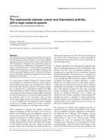
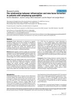
Figure 1 displays scatter plots of the expected GL (
ˆ
y
G
L
)
and the posterior mean of expected liabilities to CD and
SB (
ˆ
l
C
D
and
ˆ
l
S
B
) obtained with SMM against those
obtained with RMM. As expected, similar posterior
means of
ˆ
y

G
L
wereobtainedfromSMMandRMM
(Pearson’s correlation near 1), because the model for GL
is not affected by the s tructure imposed in recursive
models. The correlation between the posterior means of
liability to CD from the SMM and each of the RMM
were also close to 1, with very slight differences between
them. However, a weaker association was found between
the posterior means of liabilities to SB estimated with
SMM and each of the RMM (Pearson’ s correlations
around 0.69-0.70).
Figure 2 shows the plots of the posterior mean of the
expected GL and liabilities to CD and SB obtained with
one of the RMM against those of the remaining recursive
models. Again, the posterior means of the esti mated phe-
notype of GL and the liabilities to CD o btained from the
different RMM were similar, with correlations of ≥ 0.99.
Estimated liabilities from RMM2 and RMM3 were also
similar, with a correlation of 0.99. Correlations between
estimates from RMM1 and RMM2 and estimates from
RMM1 and RMM3 were slightly lower (0.98).
Table 2 shows the average MSE and Pearson’s correla-
tion between fitted and observed phenotypes of GL, CD
and SB, by model. The goodness of fit measures did not
change across models, with differences at the third deci-
mal place.
The differences observed between the posterior mean
liabilities to SB from SMM and those from RMM (see
Figure 1) did not occur when the goodness of fit of

these models was evaluated in terms of MSE and Pear-
son’ s correlation between predicted and observed SB
score.
Predictive ability
Table 3 presents the average MSE and Pearson’s correla-
tion between predicted and obser ved phenotypes of GL,
CD and SB, by model. Both RMM and SMM had simi-
lar predictive abilities of GL and CD. Regarding SB, the
model with best predictive ability was RMM1, with a
2.2% higher Pearson’s correlation than other RMM. The
differences in predictive ability among RMM were very
small.
de Maturana et al. Genetics Selection Evolution 2010, 42:1
/>Page 6 of 9
The negligible differences in terms of goodness of fit
and predictive ability between models might be
explained by the small differences in estimated genetic
correlations between SMM (off diagonals of
G
s
0
,
G
mgs
0
and
G
smg
s
0

) and RMM (off diagonals of
G
k
*
).
The larger differences observed in correlations between
contemporary groups for GL and liability to SB and
between liabilities to CD and SB, as well as their coun-
terparts between residual effects from SMM and RMM,
were not reflected in goodness of fit and predictive
ability. Thus, a very restrictive model (RMM3, with 26
parameters) provided similar fit and predictive ability a s
less parsimonious models.
Conclusions
This paper illustrates how SEM can be used to achieve
parameterizations with different levels of complexity
that represent different genetic models. For example,
recursive relationships can be used to generate models
Figure 1 Plots and Pearson’ s correlations between the posterior means of expected gestation length (
ˆ
y
G
L
) and of ex pected
liabilities to calving difficulty (
ˆ
l
C
D
) and stillbirth (

ˆ
l
S
B
) obtained with standard mixed models SMM versus those obtained with
recursive mixed models (RMM)
de Maturana et al. Genetics Selection Evolution 2010, 42:1
/>Page 7 of 9
Table 3 Predictive ability of standard (SMM) and
recursive mixed models from the analyses of cross-
validation subsets
Comparison criteria Model
a,b
SMM RMM1 RMM2 RMM3
GL
Average mean squared error 19.559 19.559 19.558 19.558
Pearson’s correlation 0.424 0.424 0.424 0.424
CD
Average mean squared error 0.824 0.823 0.824 0.823
Pearson’s correlation 0.448 0.450 0.449 0.450
SB
Average mean squared error 0.111 0.111 0.111 0.111
Pearson’s correlation 0.150 0.172 0.170 0.170
a
Boldface numbers indicate the best performance by criterion of comparison;
b
RMM1: recursive mixed model (RMM) assuming that the relationship
between residuals is due to the recursive relationships between the gestation
length (GL) phenotype and the liabilities to calving difficulty (CD) and stillbirth
(SB); RMM2: RMM assuming that the relationships both between residuals and

between herd-years are due to the recursive relationships between the
phenotype of GL and the liabilities to CD and SB; RMM3: recursive mixed
model assuming that phenotypic correlations of the system are uniquely
caused by the recursiveness
Figure 2 Plots and Pearson’s correlations between the posterior means of expected gestation length (
ˆ
y
G
L
) and of expected liabilities
to calving difficulty (
ˆ
l
C
D
) and stillbirth (
ˆ
l
S
B
) obtained with the recursive mixed models (RMM)
Table 2 Goodness of fit criteria for standard (SMM) and
recursive (RMM) mixed models
Comparison criteria Model
a,b
SMM RMM1 RMM2 RMM3
GL
Mean squared error 18.717 18.717 18.716 18.715
Pearson’s correlation 0.465 0.465 0.465 0.465
CD

Mean squared error 0.788 0.791 0.791 0.791
Pearson’s correlation 0.487 0.485 0.486 0.486
SB
Mean squared error 0.108 0.109 0.109 0.109
Pearson’s correlation 0.246 0.243 0.244 0.243
a
Boldface numbers indicate the best performance in goodness of fit, by
criterion of comparison;
b
RMM1: recursive mixed model assuming that the
relationship between residuals is due to the recursive relationships between
the gestation length (GL) phenotype and the liabilities to calving difficulty
(CD) and stillbirth (SB); RMM2: RMM assuming that the relationships both
between residuals and between herd-years are due to the recursive
relationships between the phenotype of GL and the liabilities to CD and SB;
RMM3: recursive mixed model assuming that phenotypic correlations of the
system are uniquely caused by the recursiveness
de Maturana et al. Genetics Selection Evolution 2010, 42:1
/>Page 8 of 9
in which the genetic parameters are themselves subject
to genetic variation.
The applications examined in this study suggest the
plausibility of a recursive effect from GL onto CD and
SB. Also, as reported in previous studies, this relation-
ship is not linear. The fact that the most restrictive
model (RMM3), which assumes that the only cause of
correlation is phenotypic recursion, performs as well as
the others indicates that the recursion may be an impor-
tant cause of the observed genetic and environmental
correlations.

Additional file 1: Table S1 - Posterior means (standard deviations) of
direct (d) and maternal (m) heritabilities of calving traits. Table S2 -
Posterior means (standard deviations) of the genetic correlations, for
gestations within 261-267 d. Table S3 - Posterior means (standard
deviations) of the genetic correlations, for gestations within 268-273 d.
Table S4 - Posterior means (standard deviations) of the genetic
correlations, for gestations within 274-279 d. Table S5 - Posterior means
(standard deviations) of the genetic correlations, for gestations within
280-291 d. Table S6 - Posterior means (standard deviations) of
correlations between contemporary (h) groups and residual (e) effects.
Click here for file
[ />S1.DOC ]
Acknowledgements
The authors would like to acknowledge the National Association of Animal
Breeders (Columbia, MO) for providing data for the present study, as well as
for providing partial financial support for Dr. Kent Weigel. Research was also
supported by the Wisconsin Agriculture Experiment Station and by grant
NSF-DMS-044371. We thank an anonymous referee for helpful comments.
Author details
1
Department of Animal Sciences, University of Wisconsin, Madison, 53706,
USA.
2
Departamento de Mejora Genética Animal, INIA, Carretera de La
Coruña km 7.5, 28040 Madrid, Spain.
3
Department of Dairy Science,
University of Wisconsin, Madison, 53706, USA.
4
Department of Biostatistics

and Medical Informatics, University of Wisconsin, Madison, 53706, USA.
Authors’ contributions
ELM conceived, carried out the study and wrote the manuscript; GC
conceived, supervised the study and wrote the manuscript; XLW developed
the software and revised the manuscript; DG, KW and GR helped to
coordinate the study, provided critical insights and revised the manuscript.
Competing interests
The authors declare that they have no competing interests.
Received: 20 May 2009
Accepted: 25 January 2010 Published: 25 January 2010
References
1. Wright S: The method of path coefficients. The Annals of Mathematical
Statistics 1934, 5(3):161-215.
2. Gianola D, Sorensen D: Quantitative genetic models for describing
simultaneous and recursive relationships between phenotypes. Genetics
2004, 167:1407-1424.
3. de los Campos G, Gianola D, Boettcher P, Moroni P: A structural equation
model for describing relationships between somatic cell score and milk
yield in dairy goats. J Anim Sci 2006, 84:2934-2941.
4. de los Campos G, Gianola D, Heringstad B: A structural equation model
for describing relationships between somatic cell score and milk yield in
first-lactation dairy cows. J Dairy Sci 2006, 89:4445-4455.
5. Varona L, Sorensen D, Thompson R: Analysis of litter size and average
litter weight in pigs using a recursive model. Genetics 2007,
177:1791-1799.
6. López de Maturana E, Legarra A, Varona L, Ugarte E: Analysis of fertility
and dystocia in Holsteins using recursive models to handle censored
and categorical data. J Dairy Sci 2007, 90:2012-2024.
7. Wu X-L, Heringstad B, Chang YM, de los Campos G, Gianola D: Inferring
relationships between somatic cell score and milk yield using

simultaneous and recursive models. J Dairy Sci 2007, 90:3508-3521.
8. Hershberger SL, Marcoulides GA, Parramore MM: Structural equation
modeling. Applications in ecological and evolutionary biology Cambrigde, UK:
The press sindicate of the University of Cambridge 2003.
9. Bollen KA: Structural equations with latent variables. NewYork 1989.
10. López de Maturana E, Wu X-L, Gianola D, Weigel KA, Rosa GJM: Exploring
biological relationships between calving traits in primiparous cattle with
a Bayesian recursive model. Genetics 2009, 181:277-287.
11. Willham RL: The role of maternal effects in animal breeding: III.
Biometrical aspects of maternal effects in animal breeding. J Anim Sci
1972, 35:1288-1292.
12. Kriese LA, Bertrand JK, Benyshek LL: Age adjustment factors, heritabilities
and genetic correlations for scrotal circumference and related growth
traits in Hereford and Brangus bulls. J Anim Sci 1991, 69:478-489.
13. Korsgaard IR, Andersen AH, Sorensen D: A useful reparameterisation to
obtain samples from conditional inverse Wishart distributions. Genet Sel
Evol 1999, 31:177-181.
14. Sorensen DA, Gianola D: Likelihood, Bayesian, and MCMC Methods in
Quantitative Genetics Springer-Verlag New York, Inc., 175 Fifth Avenue, New
York 2002.
15. Heringstad B, Chang YM, Svendsen M, Gianola D: Genetic analysis of
calving difficulty and stillbirth in Norwegian Red cows. J Dairy Sci 2007,
90:3500-3507.
16. Hansen M, Lund MS, Pedersen J, Christensen LG: Gestation length in
Danish Holsteins has weak genetic associations with stillbirth, calving
difficulty, and calf size. Livest Prod Sci 2004, 91:23-33.
17. Steinbock L, Näsholm A, Berglund B, Johansson K, Philipsson J: Genetic
effects on stillbirth and calving difficulty in Swedish Holsteins at first
and second calving. J Dairy Sci 2003, 86:2228-2235.
18. Wiggans GR, Misztal I, Van Tassell CP: Calving ease (co)variance

conponents for a sire-maternal grandsire threshold model. J Dairy Sci
2003, 86:1845-1848.
19. Cole JB, Wiggans GR, VanRaden PM, Miller RH: Stillbirth (co)variance
components for a sire-maternal grandsire threshold model and
development of a calving ability index for sire selection. J Dairy Sci 2007,
90:2489-2496.
20. Berger JO, Pericchi LR: The Intrinsic Bayes Factor for Model Selection and
Prediction. J Am Stat Assoc 1996, 91:109-122.
doi:10.1186/1297-9686-42-1
Cite this article as: de Maturana et al.: Modeling relationships between
calving traits: a comparison between standard and recursive mixed
models. Genetics Selection Evolution 2010 42:1.
Submit your next manuscript to BioMed Central
and take full advantage of:
• Convenient online submission
• Thorough peer review
• No space constraints or color figure charges
• Immediate publication on acceptance
• Inclusion in PubMed, CAS, Scopus and Google Scholar
• Research which is freely available for redistribution
Submit your manuscript at
www.biomedcentral.com/submit
de Maturana et al. Genetics Selection Evolution 2010, 42:1
/>Page 9 of 9