Báo cáo y học: "Coverage and error models of protein-protein interaction data by directed graph analysis" pptx
Bạn đang xem bản rút gọn của tài liệu. Xem và tải ngay bản đầy đủ của tài liệu tại đây (770.06 KB, 14 trang )
Genome Biology 2007, 8:R186
comment reviews reports deposited research refereed research interactions information
Open Access
2007Chianget al.Volume 8, Issue 9, Article R186
Method
Coverage and error models of protein-protein interaction data by
directed graph analysis
Tony Chiang
*†
, Denise Scholtens
‡
, Deepayan Sarkar
†
, Robert Gentleman
†
and Wolfgang Huber
*
Addresses:
*
EMBL, European Bioinformatics Institute, Wellcome Trust Genome Campus, Hinxton, Cambridge, CB10 1SD, UK.
†
Fred
Hutchinson Cancer Research Center, Computational Biology Group, Fairview Avenue North, Seattle, WA 98109-1024, USA.
‡
Northwestern
University, Department of Preventive Medicine, N Lake Shore Drive, Chicago, IL 60611-4402, USA.
Correspondence: Tony Chiang. Email:
© 2007 Chiang et al.; licensee BioMed Central Ltd.
This is an open access article distributed under the terms of the Creative Commons Attribution License ( which
permits unrestricted use, distribution, and reproduction in any medium, provided the original work is properly cited.
Error rates in protein-protein interaction data<p>Directed graph and multinomial error models were used to assess and characterize the error statistics in all published large-scale data-sets for <it>Saccharomyces cerevisiae</it></p>
Abstract
Using a directed graph model for bait to prey systems and a multinomial error model, we assessed
the error statistics in all published large-scale datasets for Saccharomyces cerevisiae and
characterized them by three traits: the set of tested interactions, artifacts that lead to false-positive
or false-negative observations, and estimates of the stochastic error rates that affect the data.
These traits provide a prerequisite for the estimation of the protein interactome and its modules.
Background
Within the past decade a large amount of data on protein-pro-
tein interactions in cellular systems has been obtained by the
high-throughput scaling of technologies, such as the yeast
two-hybrid (Y2H) system and affinity purification-mass spec-
trometry (AP-MS) [1-15]. This opens the possibility for molec-
ular and computational biologists to obtain a comprehensive
understanding of cellular systems and their modules [16].
There are many references in the literature, however, to the
apparent noisiness and low quality of high-throughput pro-
tein interaction data. Evaluation studies have reported dis-
crepancies between the datasets, large error rates, lack of
overlap, and contradictions between experiments [17-30].
The interpretation and integration of these large sets of pro-
tein interaction data represents a grand challenge for compu-
tational biology.
In essence, inference on the existence of an interaction
between two proteins is made based on the measured data,
and such inference can either be right or wrong. Most publicly
available data are stored as positive measured results, and
therefore most analyses have employed the most obvious
method to infer interactions; a positive observation indicates
an interaction, whereas a negative observation or no observa-
tion does not. This method, although useful and sometimes
unavoidable, does not make use of other indicators for the
presence or absence of interactions.
The most useful and yet seldom used indicator is the informa-
tion about which set of interactions were tested. As men-
tioned, most studies report positively measured interactions
but few report the negative measurements. It is quite often
the case that untested protein pairs and negative measure-
ments are not distinguished. A second indicator of the pres-
ence of an interaction is reciprocity. Bait to prey systems
allow for the testing of an interaction between a pair of pro-
teins in two directions. If bi-directionally tested, we anticipate
the result as both positive or both negative. Failure to attain
reciprocity indicates some form of error. A third indicator is
the type of interaction being assayed; direct physical
Published: 10 September 2007
Genome Biology 2007, 8:R186 (doi:10.1186/gb-2007-8-9-r186)
Received: 12 March 2007
Revised: 26 May 2007
Accepted: 10 September 2007
The electronic version of this article is the complete one and can be
found online at />R186.2 Genome Biology 2007, Volume 8, Issue 9, Article R186 Chiang et al. />Genome Biology 2007, 8:R186
interactions must be differentiated from indirect interac-
tions, and this difference plays an important role in inference.
In the Y2H system, two proteins are modified so that a phys-
ical interaction between the two can reconstitute a function-
ing transcription factor. In AP-MS, a single protein is chosen
and modified, and each pull-down detects proteins that are in
some complex with the selected one but may not necessarily
directly interact with the chosen protein.
Restricting our attention to bi-directionally tested interac-
tions, we can use a binomial model to identify proteins that
either find a disproportionate number of prey relative to the
number of baits that find them or vice versa. For the AP-MS
experiments, there is an association between whether a pro-
tein exhibits this discrepancy and its relative abundance in
the cell. For the Y2H system, analyses conducted separately
by Walhout and coworkers [31], Mrowka and colleagues [19],
and Aloy and Russell [32] have reported on this type of arti-
fact and have discussed a relationship between it and some
bait proteins' propensity to act alone as activators of the
reporter gene. Our methods provide a simple test to identify
proteins that are probably affected by such systematic errors.
Such diagnostics can aid in the interpretation of the data and
in the design of future experiments. By restricting attention to
proteins that are not seen to be affected by this artifact, we
can refine the error modeling and the subsequent biologic
analysis.
Results and discussion
Tested interactions and their representations
In the Y2H system, the bait is the protein tagged with the
DNA binding domain, and the prey is the hybrid with the acti-
vation domain. Only those constructs that result in a func-
tional fusion protein will be tested as bait or as a prey. In AP-
MS, a piece of DNA encoding a tag is inserted into a protein-
coding gene, so that yeast cells express the tagged protein.
These are the baits. The prey are unmodified proteins
expressed under the conditions of the experiment. The set of
tested baits, even in experiments intended to be genome
wide, can be quite restricted. For example, Gavin and cowork-
ers [10] designed their experiment to employ the 6,466 open
reading frames that were at that time annotated with the Sac-
charomyces cerevisiae genome, but successfully obtained
tandem affinity purifications for 1,993 of those. The remain-
ing 4,473 (69%) failed at various stages, because, for example,
the tagged protein failed to express or the bands resulting
from the gel electrophoresis were not well separated.
It is difficult to give an accurate enumeration of the sets of
tested baits and tested prey in an experiment, and often the
published data do not contain sufficient detail to allow iden-
tification of these sets. As a proxy, we introduce the concepts
of viable baits and viable prey; the first is the set of baits that
were reported to have interacted with at least one prey, and
the latter is similarly defined. These quantities are unambig-
uously obtained from the reported data and provide reasona-
ble surrogate estimates for what are the tested baits and
tested prey. The set of ordered pairs, one being a viable bait
and the other a viable prey, are interactions for which we have
a level of confidence that were experimentally tested and
could, in principle, have been detected. The failure to detect
an interaction between a viable bait and a viable prey is
informative, whereas the absence of an observed interaction
between an untested bait and prey is not. This approach over-
emphasizes positive interactions; potentially, valid data on
tested proteins that have truly no interactions with any other
tested protein will be discarded.
Protein interactions have been generally modeled by ordinary
graphs [33]. The proteins correspond to the nodes of the
graph, and edges between protein pairs indicate an interac-
tion (either physical interaction or complex co-membership).
For measured data from bait to prey systems, protein pairs
are ordered (b,p) to distinguish a bait b from a prey p. There
are three types of relationships between protein pairs of an
experimental dataset: tested with an observed interaction,
tested with no observed interaction, and untested. An ade-
quate representation for this type of datum would be a
directed graph with edge attributes. A directed edge (b,p)
+
signals testing with an observed interaction, whereas a
directed edge (b,p)
-
signals testing without an observed inter-
action. Interactions between proteins that are not adjacent
were not tested. In those cases in which all protein pairs were
reciprocally tested, we can suppress the (b,p)
-
edges, and a
directed graph (digraph) is an adequate representation.
As mentioned above, information on which protein pairs
were tested for an interaction is rarely explicitly reported, and
so we represent the current data by a directed graph with
node attributes. Using viability as a proxy for testing, the
nodes with non-zero out-degree are presumed to be the set of
viable baits, and similarly the nodes with non-zero in-degree
are presumed to be the viable prey. Isolated nodes become
identified as the set of untested proteins (both as bait and
prey). We make use of such a di-graph data structure in this
report (Figure 1).
Interactome coverage
Given the experimental data, one can partition the proteins
into four different sets: viable bait only (VB), viable prey only
(VP), viable bait/prey (VBP), and the untested proteins. Fig-
ure 2 shows these proportions of the yeast genome as meas-
ured by each experiment. For most experiments, relatively
large portions of the proteome were untested by the assay
(gray area), thereby rendering an incomplete picture of the
overall interactome [18,21,25,34].
We considered whether the sets of viable bait and viable prey
exhibited a coverage bias in the experimental assays. Apply-
ing a conditional hypergeometric test [35] to the terms within
the cellular component branch of Gene Ontology (GO), we
Genome Biology 2007, Volume 8, Issue 9, Article R186 Chiang et al. R186.3
comment reviews reports refereed researchdeposited research interactions information
Genome Biology 2007, 8:R186
found that proteins annotated to categories such as nucleus
(primarily Y2H), cytoplasm, and protein complex were over-
represented among the viable protein population relative to
the yeast genome. This is not surprising because both Y2H
and AP-MS assay two kinds of interactions in protein com-
plexes. The Y2H technology is more successful in generating
viable proteins within the nucleus because this is the cellular
location where the test is performed, and so native proteins
tend to work more successfully.
The conditional hypergeometric tests can also identify por-
tions of the cellular component missed by either Y2H or AP-
MS. For the Y2H technology, terms associated with mito-
chondrion, ribosome, and integral to membrane were under-
represented by viable proteins. Like the Y2H systems, the via-
ble proteins from AP-MS assays were also under-represented
with respect to terms associated with mitochondrion and
integral to membrane, but instead of ribosome AP-MS
showed under-representation in vacuole. These under-repre-
sented categories are limited by the technologies because all
datasets were derived before progress had been made to
probe membrane-bound proteins.
Every dataset, whether Y2H or AP-MS, exhibited under-rep-
resentation for the term cellular component unknown. One
possible explanation for this phenomenon can be attributed
to the correlation between different technologies. It seems
that proteins that are problematic in the Y2H and AP-MS sys-
tems might also be problematic in systems to determine their
cellular localization. Ultimately, further experiments are
needed to determine why certain GO categories are under-
represented. The hypergeometric analysis on each dataset
can be found in the Additional data files.
These findings point to the fact that the subset of the interac-
tome is either non-randomly sampled or non-randomly cov-
ered by the experiment. Either effect limits the type of
inference that can be conducted on the resulting data. For
instance, inference on statistics such as the degree distribu-
tion or the clustering coefficient of the overall graph is less
meaningful as long as the direction and magnitude of the cov-
erage or sampling biases are not well understood [20,36,37].
Systematic bias: per protein and experiment wide
The interactions between VBP proteins were tested in both
directions, and a surprising yet useful observation is that
there is a large number of unreciprocated edges in the data
Measured protein interaction data are represented by a directed graphFigure 1
Measured protein interaction data are represented by a directed graph.
The graph shows the interaction data between four selected proteins from
the report by Krogan and coworkers [11]. The bi-directional edge
between the ATPase SSA1 and the translational elongation factor TEF2
indicates that either one as a bait pulled down the other one as a prey.
The directed edge from RPC82, a subunit of RNA polymerase III, to SSA1
indicates that RPC82 as a bait pulled down SSA1, but not vice versa.
Another unreciprocated edge goes from the phosphatase PHO3 to TEF2.
An investigation of the dataset shows that PHO3, which localizes in the
periplasmatic space, was not reported in any interaction as a prey,
whereas RPC82C was. In the interpretation of the data, we would have
most confidence that there is a real interaction between SSA1 and TEF2.
We can differentiate between the two unreciprocated interactions; the
one between RPC82C and SSA1 has been bi-directionally tested, but only
found once, whereas the other one has only been uni-directionally tested
and found.
SSA1PHO3
TEF2
RPC82C
Proportions of proteins sampled across datasetsFigure 2
Proportions of proteins sampled across datasets. This bar chart shows the
proportion of proteins sampled either as a viable bait (VB), a viable prey
(VP), or as both (VBP). With the exception of the data report by Krogan
and coworkers [11], the other 11 datasets show large portions of the
yeast genome that did not participate in any positive observations.
Without additional information, there is little we can do to elucidate
whether these proteins were tested but inactive for all tests, or whether
these proteins were not tested.
Number of proteins
Cagney 2001
Tong 2002
Zhao 2005
Krogan 2004
Uetz 2000−2
ItoCore 2001
Uetz 2000−1
Gavin 2002
Ho 2002
Hazbun 2003
Gavin 2006
ItoFull 2001
Krogan 2006
0 2,000 4,000 6,000
Viable bait only
Both viable prey and bait
Viable prey only
Absent
R186.4 Genome Biology 2007, Volume 8, Issue 9, Article R186 Chiang et al. />Genome Biology 2007, 8:R186
[32]. These unreciprocated interactions can be used to under-
stand better the experimental errors.
Each VBP protein p has n
p
unreciprocated edges, and under
the assumption of randomness we expect the number of unre-
ciprocated in-edges and out-edges to be similar. More pre-
cisely, under the assumption that the direction of the edge is
random, the number of unreciprocated in-edges is distrib-
uted as the number of heads obtained by tossing a fair coin n
p
times. Based on this coin tossing model, we used a per protein
binomial error model (see Materials and methods, below) to
test the statistical significance for the number of unrecipro-
cated in-edges (heads) against the number unreciprocated
out-edges (tails). Figure 3 shows a partition of the VBP pro-
teins from the data of Krogan and coworkers [11] based on the
two-sided statistical test derived from the binomial model
with a P value threshold of 0.01. Those proteins falling out-
side the diagonal band are considered to be affected by a sys-
tematic bias.
It is interesting to note that the proportion of VBP proteins
identified by the binomial error model as potentially affected
by bias is quite small for the Y2H experiments and the smaller
scale AP-MS experiments (<3%), whereas the two larger scale
AP-MS experiments showed relatively greater proportions
(>14%). It is equally important to note that although these
proportions still constitute a minority of VBP proteins, these
proteins (within the large-scale AP-MS experiments) partici-
pate in a relatively large number of observed interactions,
most of which are unreciprocated.
Having identified sets of proteins that are likely to have been
affected by this systematic bias, we considered whether these
proteins could be associated with biologic properties. To this
end, we fit logistic regression models (Additional data files) to
predict this effect, and in the AP-MS system we found evi-
dence that the codon adaptation index (CAI) and protein
abundance are associated with the highly unreciprocated in-
degree of VBP proteins (proteins that were found by an excep-
tionally high number of baits relative to the number of prey
they found themselves when tested as baits). The CAI is a per-
gene score that is computed from the frequency of the usage
of synonymous codons in a gene's sequence, and can serve as
a proxy for protein abundance [38].
To visualize the association between such proteins and CAI,
we plotted diagrams of the adjacency matrix. If the value of
CAI is associated with the tendency of a protein to have a large
number of unreciprocated edges, then we should see a pattern
in the adjacency matrix when the rows and columns are
ordered by ascending CAI values. We do this for the data
reported by Gavin and coworkers [10] in Figure 4. We see a
dark vertical band in Figure 4b representing a relatively high
volume of prey activity. There is no corresponding horizontal
band in Figure 4a, which suggests that the relationship of CAI
to the AP-MS system is primarily reflected in a protein's in-
degree.
Next, we standardized the in-degree for each protein by cal-
culating its z-score (see Materials and methods, below) and
then plotted the distributions of these z-scores by their den-
sity estimates. Four experiments appeared to exhibit particu-
larly distinct distributions (Ito-Full, Ito-Core, Gavin et al.
2006, and Krogan et al. 2006; Figure 5) [1,10,11]. The Ito-Full
[1] dataset shows the largest mean (approximately two to four
times the mean of the other Y2H distributions). This is con-
sistent with reports that there were many auto-activating
baits in the Ito-Full datasets [32]; if a relatively small number
of baits auto-activate, resulting in the cell's expression of the
reporter gene, then this artificially increases the number of
in-edges for a large number of prey proteins. Auto-activation
would cause a shift in the z-score distribution in the positive
direction. This effect is not seen in the Ito-Core data.
Although Ito and coworkers [1] tried to eliminate systematic
errors by generating the Ito-Core subset of interactions, it is
noteworthy to recall that they only used reproducibility as a
criterion for validation without considering reciprocity.
Consequently, almost half of the reciprocated interactions
Two-sided binomial test on the data from Krogan and coworkers [11]Figure 3
Two-sided binomial test on the data from Krogan and coworkers [11].
The scatter-plot shows (o
p
,i
p
) for each p ∈ VBP from the report by Krogan
and coworkers [11] (axes are scaled by the square root). The proteins
that fall outside of the diagonal band exhibit high asymmetry in
unreciprocated degree. This figure shows a graphical representation of a
two-sided binomial test. The points above and below the diagonal band
are proteins for which we reject the null hypothesis that the distribution
of unreciprocated edges is governed by B(n
p
, ). For the purpose of
visualization, small random offsets were added to the discrete coordinates
of the data points by the R function jitter. VBP, viable bait/prey.
●
●
●
●
●
●
●
●
●
●
●
●
●
●
●
●
●
●
●
●
●
●
●
●
●
●
●
●
●
●
●
●
●
●
●
●
●
●
●
●
●
●
●
●
●
●
●
●
●
●
●
●
●
●
●
●
●
●
●
●
●
●
●
●
●
●
●
●
●
●
●
●
●
●
●
●
●
●
●
●
●
●
●
●
●
●
●
●
●
●
●
●
●
●
●
●
●
●
●
●
●
●
●
●
●
●
●
●
●
●
●
●
●
●
●
●
●
●
●
●
●
●
●
●
●
●
●
●
●
●
●
●
●
●
●
●
●
●
●
●
●
●
●
●
●
●
●
●
●
●
●
●
●
●
●
●
●
●
●
●
●
●
●
●
●
●
●
●
●
●
●
●
●
●
●
●
●
●
●
●
●
●
●
●
●
●
●
●
●
●
●
●
●
●
●
●
●
●
●
●
●
●
●
●
●
●
●
●
●
●
●
●
●
●
●
●
●
●
●
●
●
●
●
●
●
●
●
●
●
●
●
●
●
●
●
●
●
●
●
●
●
●
●
●
●
●
●
●
●
●
●
●
●
●
●
●
●
●
●
●
●
●
●
●
●
●
●
●
●
●
●
●
●
●
●
●
●
●
●
●
●
●
●
●
●
●
●
●
●
●
●
●
●
●
●
●
●
●
●
●
●
●
●
●
●
●
●
●
●
●
●
●
●
●
●
●
●
●
●
●
●
●
●
●
●
●
●
●
●
●
●
●
●
●
●
●
●
●
●
●
●
●
●
●
●
●
●
●
●
●
●
●
●
●
●
●
●
●
●
●
●
●
●
●
●
●
●
●
●
●
●
●
●
●
●
●
●
●
●
●
●
●
●
●
●
●
●
●
●
●
●
●
●
●
●
●
●
●
●
●
●
●
●
●
●
●
●
●
●
●
●
●
●
●
●
●
●
●
●
●
●
●
●
●
●
●
●
●
●
●
●
●
●
●
●
●
●
●
●
●
●
●
●
●
●
●
●
●
●
●
●
●
●
●
●
●
●
●
●
●
●
●
●
●
●
●
●
●
●
●
●
●
●
●
●
●
●
●
●
●
●
●
●
●
●
●
●
●
●
●
●
●
●
●
●
●
●
●
●
●
●
●
●
●
●
●
●
●
●
●
●
●
●
●
●
●
●
●
●
●
●
●
●
●
●
●
●
●
●
●
●
●
●
●
●
●
●
●
●
●
●
●
●
●
●
●
●
●
●
●
●
●
●
●
●
●
●
●
●
●
●
●
●
●
●
●
●
●
●
●
●
●
●
●
●
●
●
●
●
●
●
●
●
●
●
●
●
●
●
●
●
●
●
●
●
●
●
●
●
●
●
●
●
●
●
●
●
●
●
●
●
●
●
●
●
●
●
●
●
●
●
●
●
●
●
●
●
●
●
●
●
●
●
●
●
●
●
●
●
●
●
●
●
●
●
●
●
●
●
●
●
●
●
●
●
●
●
●
●
●
●
●
●
●
●
●
●
●
●
●
●
●
●
●
●
●
●
●
●
●
●
●
●
●
●
●
●
●
●
●
●
●
●
●
●
●
●
●
●
●
●
●
●
●
●
●
●
●
●
●
●
●
●
●
●
●
●
●
●
●
●
●
●
●
●
●
●
●
●
●
●
●
●
●
●
●
●
●
●
●
●
●
●
●
●
●
●
●
●
●
●
●
●
●
●
●
●
●
●
●
●
●
●
●
●
●
●
●
●
●
●
●
●
●
●
●
●
●
●
●
●
●
●
●
●
●
●
●
●
●
●
●
●
●
●
●
●
●
●
●
●
●
●
●
●
●
●
●
●
●
●
●
●
●
●
●
●
●
●
●
●
●
●
●
●
●
●
●
●
●
●
●
●
●
●
●
●
●
●
●
●
●
●
●
●
●
●
●
●
●
●
●
●
●
●
●
●
●
●
●
●
●
●
●
●
●
●
●
●
●
●
●
●
●
●
●
●
●
●
●
●
●
●
●
●
●
●
●
●
●
●
●
●
●
●
●
●
●
●
●
●
●
●
●
●
●
●
●
●
●
●
●
●
●
●
●
●
●
●
●
●
●
●
●
●
●
●
●
●
●
●
●
●
●
●
●
●
●
●
●
●
●
●
●
●
●
●
●
●
●
●
●
●
●
●
●
●
●
●
●
●
●
●
●
●
●
●
●
●
●
●
●
●
●●
●
●
●
●
●
●
●
●
●
●
●
●
●
●
●
●
●
●
●
●
●
●
●
●
●
●
●
●
●
●
●
●
●
●
●
●
●
●
●
●
●
●
●
●
●
●
●
●
●
●
●
●
●
●
●
●
●
●
●
●
●
●
●
●
●
●
●
●
●
●
●
●
●
●
●
●
●
●
●
●
●
●
●
●
●
●
●
●
●
●
●
●
●
●
●
●
●
●
●
●
●
●
●
●
●
●
●
●
●
●
●
●
●
●
●
●
●
●
●
●
●
●
●
●
●
●
●
●
●
●
●
●
●
●
●
●
●
●
●
●
●
●
●
●
●
●
●
●
●
●
●
●
●
●
●
●
●
●
●
●
●
●
●
●
●
●
●
●
●
●
●
●
●
●
●
●
●
●
●
●
●
●
●
●
●
●
●
●
●
●
●
●
●
●
●
●
●
●
●
●
●
●
●
●
●
●
●
●
●
●
●
●
●
●
●
●
●
●
●
●
●
●
●
●
●
●
●
●
●
●
●
●
●
●
●
●
●
●
●
●
●
●
●
●
●
●
●
●
●
●
●
●
●
●
●
●
●
●
●
●
●
●
●
●
●
●
●
●
●
●
●
●
●
●
●
●
●
●
●
●
●
●
●
●
●
●
●
●
●
●
●
●
●
●
●
●
●
●
●
●
●
●
●
●
●
●
●
●
●
●
●
●
●
●
●
●
●
●
●
●
●
●
●
●
●
●
●
●
●
●
●
●
●
●
●
●
●
●
●
●
●
●
●
●
●
●
●
●
●
●
●
●
●
●
●
●
●
●
●
●
●
●
●
●
●
●
●
●
●
●
●
●
●
●
●
●
●
●
●
●
●
●
●
●
●
●
●
●
●
●
●
●
●
●
●
●
●
●
●
●
●
●
●
●
●
●
●
●
●
●
●
●
●
●
●
●
●
●
●
●
●
●
●
●
●
●
●
●
●
●
●
●
●
●
●
●
●
●
●
●
●
●
●
●
●
●
●
●
●
●
●
●
●
●
●
●
●
●
●
●
●
●
●
●
●
●
●
●
●
●
●
●
●
●
●
●
●
●
●
●
●
●
●
●
●
●
●
●
●
●
●
●
●
●
●
●
●
●
●
●
●
●
●
●
●
●
●
●
●
●
●
●
●
●
●
●
●
●
●
●
●
●
●
●
●
●
●
●
●
●
●
●
●
●
●
●
●
●
●
●
●
●
●
●
●
●
●
●
●
●
●
●
●
●
●
●
●
●
●
●
●
●
●
●
●
●
●
●
●
●
●
●
●
●
●
●
●
●
●
●
●
●
●
●
●
●
●
●
●
●
●
●
●
●
●
●
●
●
●
●
●
●
●
●
●
●
●
●
●
●
●
●
●
●
●
●
●
●
●
●
●
●
●
●
●
●
●
●
●
●
●
●
●
●
●
●
●
●
●
●
●
●
●
●
●
●
●
●
●
●
●
●
●
●
●
●
●
●
●
●
●
●
●
●
●
●
●
●
●
●
●
●
●
●
●
●
●
●
●
●
●
●
●
●
●
●
●
●
●
●
●
●
●
●
●
●
●
●
●
●
●
●
●
●
●
●
●
●
●
●
●
●
●
●
●
●
●
●
●
●
●
●
●
●
●
●
●
●
●
●
●
●
●
●
●
●
●
●
●
●
●
●
●
●
●
●
●
●
●
●
●
●
●
●
●
●
●
●
●
●
●
●
●
●
●
●
●
●
●
●
●
●
●
●
●
●
●
●
●
●
●
●
●
●
●
●
●
●
●
●
●
●
●
●
●
●
●
●
●
●
●
●
●
●
●
●
●
●
●
●
●
●
●
●
●
●
●
●
●
●
●
●
●
●
●
●
●
●
●
●
●
●
●
●
●
●
●
●
●
●
●
●
●
●
●
●
●
●
●
●
●
●
●
●
●
●
●
●
●
●
●
●
●
●
●
●
●
●
●
●
●
●
●
●
●
●
●
●
●
●
●
●
●
●
●
●
●
●
●
●
●
●
●
●
●
●
●
●
●
●
●
●
●
●
●
●
●
●
●
●
●
●
●
●
●
●
●
●
●
●
●
●
●
●
●
●
●
●
●
●
●
●
●
●
●
●
●
●
●
●
●
●
●
●
●
●
●
●
●
●
●
●
●
●
●
●
●
●
●
●
●
●
●
●
●
●
●
●
●
●
●
●
●
●
●
●
●
●
●
●
●
●
●
●
●
●
●
●
●
●
●
●
●
●
●
●
●
●
●
●
●
●
●
●
●
●
●
●
●
●
●
●
●
●
●
●
●
●
●
●
●
●
●
●
●
●
●
●
●
●
●
●
●
●
●
●
●
●
●
●
●
●
●
●
●
●
●
●
●
●
●
●
●
●
●
●
●
●
●
●
●
●
●
●
●
●
●
●
●
●
●
●
●
●
●
●
●
●
●
●
●
●
●
●
●
●
●
●
●
●
●
●
●
●
●
●
●
●
●
●
●
●
●
●
●
●
●
●
●
●
●
●
●
●
●
●
●
●
●
●
●
●
●
●
●
●
●
●
●
●
●●
●
●
●
●
●
●
●
●
●
●
●
●
●
●
●
●
●
●
●
●
●
●
●
●
●
●
●
●
●
●
●
●
●
●
●
●
●
●
●
●
●
●
●
●
●
●
●
●
●
●
●
●
●
0102030
0102030
n
out
n
in
1
2
Genome Biology 2007, Volume 8, Issue 9, Article R186 Chiang et al. R186.5
comment reviews reports refereed researchdeposited research interactions information
Genome Biology 2007, 8:R186
were not recorded in the Ito-Core set. Although reproducibil-
ity is a necessary condition for validation, it is insufficient
because systematic errors are often reproducible.
Among the AP-MS datasets, the data reported by both Gavin
and coworkers [10] and Krogan and colleagues [11] display
negative means. A possible interpretation of this effect can be
attributed to the abundance of the prey under the conditions
of the experimental assay. The AP-MS system is more sensi-
tive in detecting the complex co-members of a particular bait
than in the reverse. For instance, if a lowly expressed protein
p is tagged and expressed as a bait and pulls-down proteins
p
1
, ,p
k
as prey, then the reverse tagging of each protein of
p
1
, ,p
k
will have a smaller probability of finding p. Even if the
lowly abundant protein p is pulled down in the reverse tag-
ging, the mass spectrometry may fail to detect p within the
complex mixture [39,40]. Both of these observations could
explain why we observed proteins having an overall slightly
higher out-degree than in-degree, and therefore an overall
slightly negative mean for the z-score distribution.
Finally, we wished to cross-compare the systematic errors
between experiments. Only two experiments had sufficient
size to give reasonable statistical power. Thus, to compare
systematic errors of Gavin and coworkers [10] against those
of Krogan and colleagues [11], we generated two-way tables
(Tables 1 to 4; also, see Materials and methods, below).
Although the concordance is not complete, there is evidence
that overlapping sets of proteins are affected. This indicates
that both experiment specific and more general factors could
be at work, resulting in these unreciprocated edges.
Stochastic error rate analysis
There has been confusion in the literature when analyzing
error statistics, because different articles have used different
definitions for the same statistic. Proteins pairs can either
interact or not, and so the pairs themselves can be partitioned
into two distinct sets; the set of interacting pairs, I, and the set
of non-interacting pairs, I
C
. False negative (FN) interactions
and true positive (TP) interactions can only occur within the
set I, and therefore the false negative probability (P
FN
) and
the true positive probability (P
TP
) are properties on I. Simi-
larly, the false positive (P
FP
) and true negative (P
TN
) probabil-
ities are properties on I
C
[41]. These standard definitions,
along with the values n = |I| and m = |I
C
|, allow us to set up
equations for the expectation values of three random
Adjacency matrices: random versus ascending CAIFigure 4
Adjacency matrices: random versus ascending CAI. These plots present a view of the adjacency matrix for the viable bait/prey (VBP) derived from the
report from Gavin and coworkers [10]. An interaction between bait b and prey p is recorded by a dark pixel in (b,p)th position of the matrix. (a) Rows
and columns are randomly ordered; (b) rows and columns are ordered by ascending values of each protein's codon adaptation index (CAI). Contrasting
these two figures, we can ascertain that there is a relationship between bait/prey interactions and CAI. The relationship is based on proteins with large un-
reciprocated in-degree because panel b shows a dark vertical band. Had unreciprocated out-degree also been associated with CAI, then there would be a
similar horizontal band reflected across the main diagonal of the matrix.
(a) Random order
Gavin 2006
Prey
Bait
200
400
600
800
200 400 600 800
(b) Ordered by ascending CAI
Gavin 2006
Prey
Bait
200
400
600
800
200 400 600 800
R186.6 Genome Biology 2007, Volume 8, Issue 9, Article R186 Chiang et al. />Genome Biology 2007, 8:R186
variables: the number of reciprocated edges (X
1
), the number
of protein pairs between which no edge exists (X
2
), and the
number of unreciprocated edges (X
3
).
E[X
1
] = n (1 - P
FN
)
2
+ mP
FP
2
(1)
E[X
2
] = nP
FN
2
+ m(1 - P
FP
)
2
(2)
Density plots of the in-degree z-scoresFigure 5
Density plots of the in-degree z-scores. The plots show the density estimates of the in-degree z-scores for [1,10,11]. The zero line is present to distinguish
between positive and negative z-scores. The distribution reported by Ito and coworkers [1] shows a high concentration of data points that have positive
z-scores, whereas the data reported by Gavin and coworkers [10] and Krogan and colleagues [11] have maximal density for negative z. Systematic artifacts
such as auto-activators in the yeast two-hybrid (Y2H) system and protein abundance in affinity purification-mass spectrometry (AP-MS) might play a role in
off-zero mean of these density plots. Restricting to the Ito-Core set appears to eliminate the effect from the Ito-Full set.
−4 −2 0 2 4
0.00 0.15 0.30
(a) z−scores for Ito Full 2001
z
Density
−2 −1 0 1 2
0.00 0.10 0.20
(b) z−scores for Ito Core 2001
z
Density
−6 −4 −2 0 2 4 6
0.00 0.10 0.20
(c) z−scores for Gavin 2006
z
Density
−10 −5 0 5 10
0.00 0.05 0.10 0.15
(d) z−scores for Krogan 2006
z
Density
Genome Biology 2007, Volume 8, Issue 9, Article R186 Chiang et al. R186.7
comment reviews reports refereed researchdeposited research interactions information
Genome Biology 2007, 8:R186
E[X
3
] = 2nP
FN
(1 - P
FN
) + 2mP
FP
(1 - P
FP
)(3)
We recall that if N is the number of proteins, then n + m =
, which is the number of all pairs of proteins. Any two of
these three equations imply the third, and therefore there are
three unknowns and two independent equations. By the
method of moments[42], we replace the left hand side of
Equations1 to 3 with the observed values for the number of
reciprocated interactions (x
1
), for the number of reciprocally
non-interacting protein pairs (x
2
), and for the number of
unreciprocated interactions (x
3
); it follows that knowledge of
any one of (P
FP
,P
FN
,n) yields the other two through an
application of the quadratic formula (see Materials and meth-
ods, below). Otherwise, if none of these three parameters is
known from other sources, then Equations1 to 3 define a fam-
ily of solutions (a one-dimensional set of solutions in a space
of three variables; Figure 6).
The variability, or stochastic error, that affects a bait to prey
system can thus be characterized by a one-dimensional curve
in a three-dimensional space, {(P
FP
,P
FN
,n)}, which depends
on the experiment and can be estimated from the three exper-
iment-specific numbers x
1
, x
2
, and x
3
. If we can identify por-
tions of the data that appear to be affected by systematic bias,
such as that described in the preceding section, then we can
set these aside and focus the characterization of the
experimental errors on the remaining filtered set of data, typ-
ically with lower estimates for P
FP
and P
FN
.
To gain insight into the prevalence of FP and FN stochastic
errors, we calculated estimates of the expected number of FP
and FN observations using Equations 1 to 3, and present the
results in Tables 5 and 6. Table 5 considers the worst-case sce-
Table 1
Across experiment comparison of protein subsets associated
with systematic error
Not in Krogan
et al. [11]
In Krogan et al. [11]
Not in Gavin et al. [10] 624 63
In Gavin et al. [10] 31 12
P = 6.5 × 10
-4
Odds ratio = 3.82
This table compares the proteins affected by a reciprocity artifact from
the datasets of Gavin and coworkers [10] and Krogan and colleagues
[11]. Binomial tests were applied to identify the affected protein sets
within each experiment, and their overlap was assessed in the 2 × 2
contingency table. In this table, the binomial tests were applied to the
two experimental datasets independently, and only those proteins in
which the in-degree is much larger than the out-degree are considered.
Shown P value and odds ratio were calculated from the 2 × 2 table
using the hypergeometric distribution.
Table 2
Across experiment comparison of protein subsets associated
with systematic error
Not in Krogan
et al. [11]
In Krogan et al. [11]
Not in Gavin et al. [10] 480 181
In Gavin et al. [10] 40 29
P = 1.6 × 10
-2
Odds ratio = 1.92
Like Table 1, this table also compares the proteins affected by a
reciprocity artifact from the datasets of Gavin and coworkers [10] and
Krogan and colleagues [11]. The only exception is that the proteins
compared were those identified by the binomial tests as having out-
degree greater than in-degree. Compared with Table 1, the association
between the two datasets is relatively weaker in terms of both the P
value and odds-ratio.
N
2
⎛
⎝
⎜
⎞
⎠
⎟
Table 3
Across experiment comparison of protein subsets associated
with systematic error
Not in Krogan
et al. [11]
In Krogan et al. [11]
Not in Gavin et al. [10] 651 45
In Gavin et al. [10] 26 8
P = 1.8 × 10
-3
Odds ratio = 4.44
This table represents the comparison of proteins affected by a
reciprocity artifact from the datasets of Gavin and coworkers [10] and
Krogan and colleagues [11] as well. Before conducting the binomial
test, the data graphs were restricted to the nodes common to the
viable bait/prey (VBP) sets of both experiments. Again, only those
proteins identified by the binomial test in which in-degree is much
larger than the out-degree is compared. Both the P value and odds
ratio, obtained using the hypergeometric distribution, show a strong
association between the two sets of proteins.
Table 4
Across experiment comparison of protein subsets associated
with systematic error
Not in Krogan
et al. [11]
In Krogan et al. [11]
Not in Gavin et al. [10] 602 78
In Gavin et al. [10] 39 11
P = 4.1 × 10
-2
Odds ratio = 2.17
Like Table 3, this table also compares the proteins affected by a
reciprocity artifact from the datasets of Gavin and coworkers [10] and
Krogan and colleagues [11] restricted to the common viable bait/prey
(VBP) proteins. We consider those proteins identified by the binomial
test in which the out-degree is much larger than the in-degree. We
again see that the association between the proteins sets in terms of P
value and odds ratio is weaker when compared with the association
obtained from Table 3.
R186.8 Genome Biology 2007, Volume 8, Issue 9, Article R186 Chiang et al. />Genome Biology 2007, 8:R186
Figure 6 (see legend on next page)
0.000 0.005 0.010 0.015 0.020
0.0 0.2 0.4 0.6 0.8 1.0
(a) APMS − Unfiltered Data
p
FP
p
FN
Krogan 2006
Gavin 2006
Krogan 2004
Ho 2002
Gavin 2002
0.00 0.01 0.02 0.03 0.04 0.05
0.0 0.2 0.4 0.6 0.8
1.0
(b) Y2H − Unfiltered Data
p
FP
p
F
N
Ito Core 2001
Uetz 2000−2
Uetz 2000−1
Hazbun 2003
Tong 2002
Cagney 2001
Ito Full 2001
0.000 0.005 0.010 0.015 0.020
0.0
0.2
0.4 0.6
0.8
1.0
(c) APMS − filtered data
p
FP
p
FN
0.00 0.01 0.02 0.03 0.04 0.05
0.0
0.2
0.4 0.6
0.8
1.0
(d) Y2H − filtered data
p
FP
p
FN
Genome Biology 2007, Volume 8, Issue 9, Article R186 Chiang et al. R186.9
comment reviews reports refereed researchdeposited research interactions information
Genome Biology 2007, 8:R186
nario for FP errors, setting P
FN
= 0, and hence assuming that
all errors are false positives. We discuss the first row, corre-
sponding to the data of Ito-Full [1], as an example. A total of
720 proteins were not rejected in the two-sided binomial test,
and there are = 258,840 protein pairs, excluding
homomers. This gives us an upper limit for m. From the solu-
tion manifold shown in Figure 6d, we see that an estimate for
P
FP
is approximately 0.0008. From this it follows that the
expected number of unreciprocated FP interactions is 414
and of reciprocated FP interactions is 0.17. The actual data
contain 435 unreciprocated interactions and 68 reciprocated
ones. So, even in the estimated worst case, when all errors are
FP observations, reciprocated observations are still most
likely due to true interactions.
It is important to contrast the nature of the stochastic error
rates because there is confusion in the literature concerning
these statistics. From Figure 6, the solution curve gives an
estimate for the P
FP
rate at 0.0008 conditioned on the Ito-Full
VBP data and conditioned on P
FN
= 0; a similar estimate for
the Ito-Core dataset yields P
FP
at 0.0025. The reason for this
is because the number of non-interacting protein pairs in the
Geometric visualization of the solution curves from the algebraic equations 1 to 3Figure 6 (see previous page)
Geometric visualization of the solution curves from the algebraic equations 1 to 3. (a) Plot of (P
FP
,P
FN
) parameterized by n for the affinity purification-mass
spectrometry (AP-MS) datasets. (b) Curves for the yeast two-hybrid (Y2H) datasets. (c) AP-MS data filtered for the proteins that were rejected by the
binomial test for systematic bias. (d) curves for the Y2H data with the application of the analogous filters. These curves give upper bounds for the values
of (P
FP
,P
FN
) in the multinomial error model for each experiment. Each point on any of the curves represents three distinct values based on the methods of
moments restricted to the viable bait/prey (VBP) proteins: the true number of interactions between the VBP proteins, the P
FP
rate, and the P
FN
rate. If one
of these three parameters can be estimated, then the other two will also be determined.
Table 5
Estimates for the FP errors of each filtered dataset
Dataset (ref.) NmP
FP
E [Y
1
] E [Y
2
] U
obs
R
obs
ItoFull [1] 720 258,840 0.0008 414 0.17 435 68
ItoCore [1] 128 8,128 0.0025 41 0.05 43 36
Uetz et al. [6] 108 5,778 0.003 35 0.05 36 10
Gavin et al. [10] 852 362,526 0.0017 1230 1.10 1201 743
Krogan et al. [11] 1,458 1,062,153 0.0019 4,029 3.80 3945 538
Shown are the expected number of false positive (FP) errors on the filtered datasets for [1,6,10,11]. N is the number of proteins within each filtered
dataset. The values for P
FP
and m are estimated upper bounds obtained by setting P
FN
= 0 and using the solution curves of Figure 6c,d. Denote Y
1
as
the random variable for the number of unreciprocated FP observations, and Y
2
for the number of reciprocated FP observations. The variables U
obs
and R
obs
show the observed number of unreciprocated and reciprocated interactions from the data, respectively. The table implies that even in the
worst case scenario for maximal P
FP
, reciprocated edges mostly report true interactions.
Table 6
Estimates for the FN errors of each filtered dataset
Dataset (ref.) Nn P
FN
E [W
1
] E [W
2
] U
obs
R
obs
ItoFull [1] 720 1,200 0.76 438 693 435 259,132
ItoCore [1]1281000.384714438,156
Uetz et al. [6] 108 78 0.65 35 33 36 5,822
Gavin et al. [10] 852 2,429 0.44 1197 470 1,201 362,209
Krogan et al. [11] 1,458 11,744 0.80 3758 7,516 3,945 1,062,344
The expected number of false-negative (FN) errors on the filtered datasets for [1,6,10,11]. N is the number of proteins within each filtered dataset.
The values for P
FN
and n are estimated upper bounds obtained by setting P
FP
= 0 and using the solution curves of Figure 6c,d. Denote W
1
as the
random variable for the number of unreciprocated FN observations, and W
2
for the number of reciprocated FN observations. The variables U
obs
and
R
obs
show the observed number of unreciprocated and reciprocated interactions from the data, respectively. The table implies that in the worst case
scenario for P
FN
, the doubly tested, reciprocated noninteracting protein pairs do not give us a conclusive indication about the presence or absence of
an interaction. For this, more data are needed.
720
2
⎛
⎝
⎜
⎞
⎠
⎟
R186.10 Genome Biology 2007, Volume 8, Issue 9, Article R186 Chiang et al. />Genome Biology 2007, 8:R186
former is estimated to be approximately 250,000, whereas
this number is 8,000 for the latter. Table 5 shows that the
number of expected false positively identified unreciprocated
interactions for Ito-Full is 414 and for the Ito-Core is 41. Thus,
although the P
FP
rate of Ito-Full is three times smaller than
that of Ito-Core, the expected number of falsely discovered
interactions is an order of magnitude greater. Therefore, a
generic interaction contained within Ito-Core is much more
likely to be true than one from Ito-Full. Comparing the P
FP
rate from Ito-Full with the P
FP
rate from Ito-Core is unreason-
able when the underlying sets of non-interacting proteins
pairs are entirely different. The false discovery rate is more
intuitive, and this statistic has often been confused in the lit-
erature with the FP rate.
We also considered the worst-case scenario for FN errors. By
setting P
FP
= 0, we calculated the expected number of
unreciprocated and reciprocated false negatives in the
absence of FP errors. These numbers are presented in Table
6. Because of the size of P
FN
, we find that a large number of
protein pairs between which no edge was reported in either
direction may still, in truth, interact.
Ultimately, an observed unreciprocated interaction in the
data indicates that either a FP or a FN observation was made.
Computational models cannot definitively conclude which of
these two occurred, but these models indicate the magnitude
and nature of the problem and can be used to compare
experiments, because those with relatively higher error rates
should be discounted in any downstream analyses.
Conclusion
We have shown that protein interaction datasets can be char-
acterized by three traits: the coverage of the tested
interactions, the presence of biases in the assay that system-
atically affect certain subsets of proteins, and stochastic vari-
ability in the measured interactions. In turn, these three
characteristics can benefit the design of future protein inter-
action experiments.
The set of interactions tested is important because datasets
usually report positive results, but tend to be ambiguous on
the significance of the unreported interactions. Is it because
the interaction was tested and not detected, or because it was
not tested in the first place? Distinguishing the two cases is
important for inference and for integration across datasets.
For the currently available datasets from Y2H and AP-MS, a
practical estimate of what is the set of tested interactions is all
pairs of tested bait and tested prey. A comprehensive list of
tested proteins is usually not reported. We can, however,
obtain a useful approximation for the tested baits and prey
using the notion of viability. However, this assumption does
introduce some bias, especially for experiments with rela-
tively few bait proteins, because proteins that were tested but
did not interact with any bait protein will not be counted,
falsely raising the proportion of interactions. On the other
hand, when complete data are not reported the presumption
that interactions were tested, when they were not, introduces
bias in the other direction.
There has been substantial interest in cross-experiment anal-
ysis, or in integrating data from multiple sources
[19,23,24,29,30]. The possible pitfalls of naïve comparisons
between two experimental datasets are depicted in Figure 7.
The interactions in the intersection of the rectangles (red)
were tested by both; the interactions in the green and purple
areas were tested by one experiment but not the other; and
the interactions in the light gray areas were tested by neither
experiment. Any data analysis that does not keep track of
these different coverage characteristics risks being misled.
Therefore, coverage must be taken into consideration when
integrating and comparing multiple datasets. Additionally,
systematic bias due to the experimental assay affects the
detection of certain interactions between protein pairs, and
these systematic errors should be isolated from the dataset
Matrix representation on two separate bait to prey datasetsFigure 7
Matrix representation on two separate bait to prey datasets. A schematic
representation of the interactome coverage of two protein interaction
experiments. The adjacency matrix of the complete interactome is
represented by the large square. Experiment 1 covers a certain set of
proteins as baits (rows covered by the green vertical line) and as prey
(columns covered by the green horizontal line). The tested interactions
for experiment 1 are contained within the green rectangle. Similarly,
experiment 2 covers another set of proteins and tests for a set of
interactions contained in the purple rectangle. In the intersection of the
rectangles, the red area, are the bait to prey interactions tested by both
experiments, and in the union are the interactions tested by at least one of
the experiments. Note that the interactions in the light gray area were
tested by neither experiment, either because there are missing tested prey
(upper right corner) or missing tested baits (lower left corner). The
interactions in the white region are also tested by neither experiment
because both the baits and the prey were not tested.
Prey of experiment 1
Baits of experiment 1
Prey of experiment 2
Baits of experiment 2
Genome Biology 2007, Volume 8, Issue 9, Article R186 Chiang et al. R186.11
comment reviews reports refereed researchdeposited research interactions information
Genome Biology 2007, 8:R186
before the estimating the stochastic errors. Ultimately, many
more steps are still needed to integrate datasets, and we dis-
cuss a few necessary components.
If the assay system were perfect, then all bi-directionally
tested protein pairs would either be reciprocally adjacent or
not. In practice, unreciprocated edges are observed, and they
can be used to understand better the sources of error. Meas-
urement error can be divided into two categories: systematic
and stochastic. We have shown that there are proteins with an
inordinate imbalance between unreciprocated in-edges and
out-edges, and they behave in a systematically different way
when used as a bait than when found as a prey. This is an indi-
cation that the interaction data involving these proteins
contain either a large number of false positives or of false neg-
atives. Further data are needed to differentiate between these
two alternatives. The mode in which they fail is distinct from
the unspecific stochastic errors that we model via the FP and
FN rates, and hence they should be excluded from these
analyses.
It is useful to distinguish between the concepts of stochastic
and systematic measurement error. Systematic errors are due
to imperfections or biases in the experimental system, and
they occur in a correlated or reproducible manner. Stochastic
errors occur at random in an irreproducible manner; in
principle, they can be averaged out by repeating the experi-
ment often enough. There are many benefits to an analysis
that identifies and separates these two types of measurement
error. We have identified one type of systematic error in bait
to prey systems that appears to be associated with artifacts of
the technologies.
The occurrence of unreciprocated edges also points to some
of the aspects of the technologies that could be improved. In
AP-MS experiments, this artifact shows a strong association
to CAI and protein abundance. Because mass spectrometry
techniques are known to be, at times, less sensitive in
identifying proteins with low abundance in a complex mix-
ture, refinements of such methodology could potentially yield
more accurate measurements.
The methods we have described are useful for future applica-
tion of Y2H or AP-MS. Newer experiments can, and should,
take into consideration relative protein abundance when
assaying protein interactions. Besides this, the GO category
analysis for under-representation shows certain proteins and
protein complexes that do not work as intended under the
conditions of the assay system. Knowing which categories are
under-represented allows experimenters to adjust the
technologies or create new technologies (such as the Y2H test
for membrane bound proteins [43]).
These elementary questions of data pre-processing, quality
assessment, and error modeling may appear far removed
from the systems-level modeling of biologic systems. Such a
modeling, however, requires the use and integration of multi-
ple different datasets, to increase the breadth and depth of the
data compared with those from a single experiment. This can
only be done if the error statistics and possible patterns in the
errors are sufficiently understood. We believe that the meth-
ods and tools developed in this work provide a step in this
direction.
Materials and methods
Graph theory
We use a directed graph with node attributes to represent
each measured dataset. The proteins correspond to the node
set, and directed edges correspond with ordered protein pairs
of the form (b,p) showing that a bait b detects a prey p. The
node set with non-zero out-degree corresponds with the set of
viable baits, and the node set with non-zero in-degree corre-
sponds with the viable prey. We remove self-loops because we
set aside homomer relationships. The subgraph generated by
nodes that are both viable baits and viable prey will have
tested all protein pairs bi-directionally.
Protein interaction data
We investigated 12 publicly available datasets for S. cerevi-
siae, of which seven were assayed by Y2H and five were
assayed by AP-MS. We obtained [1-6,10] from the IntAct
repository [44] and [7-9,11] from their primary sources. All
datasets have two key properties: information on the bait to
prey directionality is retained; and the prey population is doc-
umented as genome wide. A table with an overview of the
datasets can be found in the Additional data files.
Statistical analysis
Binomial error model: detecting bias
The binomial error model assumes that in-degrees and out-
degrees are equally likely among unreciprocated edges of a bi-
directionally tested protein. Thus, we presume that the
number of unreciprocated out-edges for any bi-directionally
tested protein p is distributed as B(n
p
,), where n
p
is the
total number of unreciprocated edges of p. Under this hypo-
thesis, we can compute the P value for the observed measured
directed degree for each protein p. The null hypothesis is
rejected at the 0.01 threshold. Proteins for which we reject the
null hypothesis are deemed likely to be affected by a system-
atic bias in the assay.
Multinomial error model
Let N be the number of proteins in an interactome of interest,
then the total number of distinct protein pairs, excluding
homomers, is . Denote the set of all unique interacting
1
2
N
2
⎛
⎝
⎜
⎞
⎠
⎟
R186.12 Genome Biology 2007, Volume 8, Issue 9, Article R186 Chiang et al. />Genome Biology 2007, 8:R186
protein pairs among the N proteins by I and its complement
by I
C
. Recall that = n + m, where n = |I| and m = |I
C
|.
Only two of the three Equations 1 to 3 are independent, any
two of them imply the third. We parameterize the one-dimen-
sional solution manifold by n (0 ≤ n ≤ ). Relevant
solutions are those for which 0 ≤ P
FP
,P
FN
≤ 1. Consider n given,
then we can solve for P
FN
in terms of P
FP
:
Where we have defined Δ = (x
2
- m) - (x
1
- n). Here, x
1
is the
observed number of reciprocated interactions and x
2
is the
number of reciprocated non-interacting protein pairs. Mak-
ing a substitution for P
FN
in Equation 2, the problem reduces
to a quadratic equation in one parameter, P
FP
:
If we let
a = (n + m), b = (Δ - 2n), and ,
then an application of the quadratic formula gives two solu-
tions for p
FP
:
Then, substituting an estimate of P
FP
back into Equation 4
gives a solution for P
FN
. A similar argument carries through
given any one of the three parameters {n,P
FP
,P
FN
}. Thus, an
estimate of one of the parameters generates estimates of the
other two.
Conditional hypergeometric, logistic regression tests, and two-way
tables
We grouped the yeast genome into several defined subsets
(VB, VP, VBP, and those proteins appearing to be affected by
bias), and we wished to determine whether the subsets
showed over-representation/under-representation among
biologic categories such as GO, Kyoto Encyclopedia of Genes
and Genomes, and Pfam. We used the conditional hypergeo-
metric testing as described by Falcon and Gentleman [35] to
probe for such over-representation/under-representation at
a P value threshold of 0.01. A list of such GO categories and
Pfam domains can be generated by the R scripts hgGO.R and
hgPfam.R, contained with the Additional data files.
For those proteins that are affected by a systematic bias of
each experiment, we fitted a logistic regression on these sets
against 31 protein properties reported in the Saccharomyces
Genome Database [45] and set a P value threshold at 0.01.
Let S
i
be the set of proteins identified to be affected by a sys-
tematic bias in dataset i, and suppose we wish to compare S
i
against S
j
; we define two methods of generating S
i
and S
j
for
such a comparison. One method is the application of the bino-
mial test on the VBP subgraph of each dataset i exclusively to
determine each S
i
. The second method aims to streamline the
experimental conditions of i with that of j. First, we compute
X = VBP
i
∩ VBP
j
; then we apply the binomial test on the X
i
subgraph as well as the X
j
subgraph (because the edge-sets
will be different). Obtaining such subsets allows us to
generate a two-way table, T, to compare S
i
against S
j
. If the
first method is used to generate the subsets S
i
and S
j
, then we
must still restrict to X when computing T. T
(2,2)
counts |S
i
∩
S
j
|; T
(1,2)
and T
(2,1)
count |S
i
\S
j
| and |S
j
\S
i
|, respectively; and
T
(1,1)
counts | |. We can apply Fisher's exact test to
ascertain the independence of these two sets at a designated
P value threshold.
Per protein in-degree z-score and cross experimental comparisons
Let o
p
be the unreciprocated out-degree for a protein p and i
p
its unreciprocated in-degree. Then denote the number of
unreciprocated edges by n
p
= i
p
+ o
p
. Assuming the
distribution i
p
~ B(n
p
, ), we can compute the standardized
in-degree (z-score) for p:
Estimating the number of stochastic false positive/false negative
observations
We used the filtered data after setting aside proteins rejected
by the two-sided binomial tests to calculate the results pre-
sented in Tables 5 and 6. In the first case, we set P
FN
= 0, and
P
FN
is the maximal value in the solution curve shown in Figure
6. m is estimated as . The expected number of unrecip-
rocated FP observations is 2P
FP
(1 - P
FP
)m and of reciprocated
FP observations is . In the second case, we set P
FP
= 0
and obtain n from the solution curve. The expected number of
unreciprocated FN observations is 2P
FN
(1 - P
FN
)n and of
reciprocated FN observations is .
Software implementation and availability
The R/Bioconductor packages used in the statistical analysis
in this report are all available as freely distributed and open
N
2
⎛
⎝
⎜
⎞
⎠
⎟
N
2
⎛
⎝
⎜
⎞
⎠
⎟
P
n
mP
FN FP
=+
1
2
2()Δ
(4)
nmP nP n
m
n
m
x
FP FP
+
()
+−
()
++ − =
2
2
2
2
4
0Δ
Δ
(5)
c =+ −n
m
n
m
x
Δ
2
2
4
()
,
P
bb ac
a
FP 12
2
4
2
=
−± −
(6)
SS
i
c
j
c
∩
1
2
z
io
io
p
pp
pp
=
−
+
(7)
N
2
⎛
⎝
⎜
⎞
⎠
⎟
Pm
FP
2
Pn
FN
2
Genome Biology 2007, Volume 8, Issue 9, Article R186 Chiang et al. R186.13
comment reviews reports refereed researchdeposited research interactions information
Genome Biology 2007, 8:R186
source software packages with an Artistic license. They are
integrated into the R/Bioconductor environment for statisti-
cal computing and bioinformatics and run on operating sys-
tems Windows, Mac OS X, and Unix.
Abbreviations
AP-MS, affinity purification-mass spectrometry; CAI, codon
adaptation index; FN, false negative; FP, false positive; GO,
Gene Ontology; TN, true negative; TP, true positive; VB,
viable bait only; VBP, viable bait/prey; VP, viable prey only;
Y2H, yeast two-hybrid.
Authors' contributions
TC, RG and WH conceived and designed the investigations
described in this report. TC, DS and DS performed the com-
putational and statistical analyses. TC, RG and WH wrote
paper. All authors read and approved the final version of the
manuscript.
Additional data files
The following additional data are available with the online
version of this paper. Additional data file 1 demonstrates a full
end-to-end analysis of the protein interaction datasets. Addi-
tional data file 2 is the Bioconductor package ppiStats (ver-
sion 1.3.5 of 22 June 2007) in 'source' format. Additional data
file 3 is the ppiStats package in the 'Windows Binary' format.
Additional data file 1End-to-end analysis of the protein interaction datasetsProvided is a document demonstrating a full end-to-end analysis of the protein interaction datasets.Click here for fileAdditional data file 2Bioconductor package ppiStats in 'source' formatPresented is the Bioconductor package ppiStats (version 1.3.5 of 22 June 2007) in 'source' format. ppiStats contains the novel methods developed in this paper.Click here for fileAdditional data file 3Bioconductor package ppiStats in 'Windows binary' formatPresented is the Bioconductor package ppiStats in 'Windows binary' format.Click here for file
Acknowledgements
We thank Anne-Claude Gavin and Rob Russell for insightful discussions and
Jack Greenblatt for making their primary data available. We would also like
to thank Li Wang for careful reading of this manuscript. We acknowledge
funding through the Human Frontiers Science Program Research Grant
RGP0022/2005 to WH and RG.
References
1. Ito T, Chiba T, Ozawa R, Yoshida M, Hattori M, Sakaki Y: A compre-
hensive two-hybrid analysis to explore the yeast protein
interactome. Proc Natl Acad Sci USA 2001, 98:4569-4574.
2. Cagney G, Uetz P, Fields S: Two-hybrid analysis of the Saccharo-
myces cerevisiae 26S proteasome. Physiol Genomics 2001,
7:27-34.
3. Tong A, Drees B, Nardelli G, Bader G, Brannetti B, Castagnoli L,
Evangelista M, Ferracuti S, Nelson B, Paoluzi S, et al.: A combined
experimental and computational strategy to define protein
interaction networks for peptide recognition modules. Sci-
ence 2002, 295:321-324.
4. Hazbun T, Malmstrom L, Anderson S, Graczyk B, Fox B, Riffle M, Sun-
din B, Aranda J, McDonald W, CH C, et al.: Assigning function to
yeast proteins by integration of technologies. Mol Cell 2003,
12:1353-1365.
5. Zhao R, Davey M, Hsu Y, Kaplanek P, Tong A, Parsons A, Krogan N,
Cagney G, Mai D, Greenblatt J, et al.: Navigating the chaperone
network: an integrative map of physical and genetic interac-
tions mediated by the Hsp90 chaperone. Cell 2005,
120:715-727.
6. Uetz P, Giot L, Cagney G, Mansfield T, Judson R, Knight J, Lockshon
D, Narayan V, Srinivasan M, Pochart P, et al.: A comprehensive
analysis of protein-protein interactions in Saccharomyces
cerevisiae. Nature 2000, 403:623-627.
7. Gavin A, Bosche M, Krause R, Grandi P, Marzioch M, Bauer A, Schultz
J, Rick J, Michon A, Cruciat C, et al.: Functional organization of
the yeast proteome by systematic analysis of protein
complexes. Nature 2002, 415:141-147.
8. Ho Y, Gruhler A, Heilbut A, Bader G, Moore L, Adams S, Millar A,
Taylor P, Bennett K, Boutilier K, et al.: Systematic identification
of protein complexes in Saccharomyces cerevisiae by mass
spectrometry.
Nature 2002, 415:180-183.
9. Krogan N, Peng WT, Cagney G, Robinson MD, Haw R, Zhong G, Guo
X, Zhang X, Canadien V, Richards DP, Beattie BK, et al.: High-defi-
nition macromolecular composition of yeast RNA-process-
ing complexes. Mol Cell 2004, 13:225-239.
10. Gavin A, Aloy P, Grandi P, Krause R, Boesche M, Marzioch M, Rau C,
Jensen L, Bastuck S, Dumpelfeld B, et al.: Proteome survey reveals
modularity of the yeast cell machinery. Nature 2006,
440:631-636.
11. Krogan N, Cagney G, Yu H, Zhong G, Guo X, Ignatchenko A, Li J, Pu
S, Datta N, Tikuisis A, et al.: Global landscape of protein com-
plexes in the yeast Saccharomyces cerevisiae. Nature 2006,
440:637-643.
12. Giot L, Bader J, Brouwer C, Chaudhuri A, Kuang B, Li Y, Hao Y, Ooi
C, Godwin B, Vitols E, et al.: A protein interaction map of Dro-
sophila melanogaster. Science 2003, 302:1727-1736.
13. Li S, Armstrong C, Bertin N, Ge H, Milstein S, Boxem M, Vidalain P,
Han J, Chesneau A, Hao T, et al.: A map of the interactome net-
work of the metazoan C. elegans. Science 2004, 303:540-543.
14. Rual J, Venkatesan K, Hao T, Hirozane-Kishikawa T, Dricot A, Li N,
Berriz G, Gibbons F, Dreze M, Ayivi-Guedehoussou N, et al.:
Towards a proteome-scale map of the human protein-pro-
tein interaction network. Nature 2005, 437:1173-1178.
15. Stelzl U, Worm U, Lalowski M, Haenig C, Brembeck F, Goehler H,
Stroedicke M, Zenkner M, Schoenherr A, Koeppen S, et al.: A human
protein-protein interaction network: a resource for annotat-
ing the proteome. Cell 2005, 122:957-968.
16. Hartwell LH, Hopfield J, Leibler S, Murray A: From molecular to
modular cell biology. Nature 1999:47-52.
17. Walhout A, Boulton S, Vidal M: Yeast two-hybrid systems and
protein interaction mapping projects for yeast and worm.
Yeast 2000, 17:88-94.
18. Schwikowski B, Uetz P, Fields S: A network of protein-protein
interactions in yeast. Nat Biotechnol 2000, 18:1257-1261.
19. Mrowka R, Patzak A, Herzel H: Is there a bias in proteome
research? Genome Res 2001, 11:1971-1973.
20. Tucker C, Gera J, Uetz P: Towards an understanding of complex
protein networks. Trends Cell Biol 2001, 11:102-106.
21. Hazbun TR, Fields S: Networking proteins in yeast. Proc Natl Acad
Sci USA 2001, 98:4277-4278.
22. Deane C, Salwinski L, Xenarios I, Eisenberg D: Two methods for
assessment of the reliability of high throughput
observations. Mol Cell Proteomics 2002, 1:349-356.
23. Edwards A, Kus B, Jansen R, Greenbaum D, Greenblat J, Gerstein M:
Bridging structural biology and genomics: assessing protein
interaction data with known complexes. Trends Genet 2002,
18:529-536.
24. von Mering C, Krause R, Snel B, Cornell M, Oliver S, Fields S, Bork P:
Comparative assessment of large-scale data sets of protein-
protein interactions. Nature 2002, 417:399-403.
25. Thomas A, Cannings R, Monk N, Cannings C: On the structure of
protein-protein interactions networks. Biochem Soc Trans 2003,
31:1491-1496.
26. Lappe M, Holm L: Unraveling protein interaction networks
with near-optimal efficiency. Nat Biotechnol 2004, 22:98-103.
27. Poyatos J, Hurst L: How biologically relevant are interaction
based modules in protein networks. Genome Biol 2004, 5:R93.
28. Vidalain P, Boxem M, Ge H, Li S, Vidal M: Increasing specificity in
high-throughput yeast two-hybrid experiments. Methods
2004, 32:
363-370.
29. Goll J, Uetz P: The elusive yeast interactome. Genome Biol 2006,
7:223.
30. Gagneur J, David L, Steinmetz L: Capturing cellular machines by
systematic screens of protein complexes. Trends Microbiol
2006, 14:336-339.
31. Walhout A, Vidal M: A genetic strategy to eliminate self-activa-
tor baits prior to high-throughput yeast two-hybrid screens.
Genome Res 1999, 9:1128-1134.
32. Aloy P, Russell RB: Potential artefacts in protein-interaction
networks. FEBS Lett 2002, 530:253-254.
33. Stanley RP: Enumerative Combinatorics I New York, NY: Cambridge
R186.14 Genome Biology 2007, Volume 8, Issue 9, Article R186 Chiang et al. />Genome Biology 2007, 8:R186
University Press; 1997.
34. de Silva E, Thorne T, Ingram P, Agrafioti I, Swire J, Wiuf C, Stumpf MP:
The effects of incomplete protein interaction data on struc-
tural and evolutionary inferences. BMC Biol 2006, 4:39.
35. Falcon S, Gentleman R: Using GOstats to test gene lists for GO
term association. Bioinformatics 2006, 2:257-258.
36. Han J, Dupuy D, Bertin N, Cusick M, Vidal M: Effect of sampling on
topology predictions of protein-protein interaction
networks. Nat Biotechnol 2005, 23:839-844.
37. Stumpf MPH, Wiuf C: Sampling properties of random graphs:
the degree distribution. Phys Rev E Stat Nonlin Soft Matter Phys
2005, 72:036118.
38. Sharp PM, Li WH: The codon adaptation index: a measure of
directional synonymous codon usage bias, and its potential
applications. Nucleic Acid Res 1987, 15:1281-1295.
39. Domon B, Aebersold R: Mass spectrometry and protein
analysis. Science 2006, 312:212-217.
40. Aebersold R, Mann M: Mass spectrometry-based proteomics.
Nature 2003, 422:198-207.
41. Kelsey J, Whittemore A, Evans A, Thompson W: Methods in obser-
vational epidemiology. In Monographs in Epidemiology and
Biostatistics New York, NY: Oxford University Press; 1996.
42. Bickel P, Doksum K: Mathematical Statistics: Basic Ideas and Selected
Topics New Jersey: Prentice Hall; 2001.
43. Miller J, Lo R, Ben-Hur A, Desmarais C, Stagljar I, Noble W, Fields S:
Large-scale identification of yeast integral membrane pro-
tein interactions. Proc Natl Acad Sci USA 2005, 102:12123-12128.
44. Kerrien S, Alam-Faruque Y, Aranda B, Bancarz I, Bridge A, Derow C,
Dimmer E, Feuermann M, Friedrichsen A, Huntley R, et al.: IntAct:
open source resource for molecular interaction data.
Nucleic
Acids Res 2006, 35:D561-D565.
45. Saccharomyces Genome Database [stge
nome.org]