Basic Analysis Guide ANSYS phần 5 pdf
Bạn đang xem bản rút gọn của tài liệu. Xem và tải ngay bản đầy đủ của tài liệu tại đây (4.62 MB, 35 trang )
The sample below demonstrates a restart after changing boundary conditions.
/prep7
et,1,21
r,1,1,1,1,1,1,1
n,1
e,1
fini
/solu
antyp,trans
timint,off
time,.1
nsub,2
kbc,0
d,1,ux,100 ! to apply initial velocity (IC command is preferred)
solve
timint,on
ddele,1,ux ! this requires special handling by multi-frame restart
! if a reaction force exists at this dof, replace it with an equal
! force using the endstop option
time,.2
nsub,5
rescontrol,define,all,1 ! request possible restart from any substep
outres,nsol,1
solve
fini
/solu
antyp,,restart,2,3 ! this command resumes the .rdb database created at the start of solution
! (restart from substep 3)
ddele,1,ux ! re-specify boundary condition deleted during solution
solve
fini
/post26
nsol,2,1,ux
prvar,2 ! results show constant velocity through restart
fini
/exit
Note
If you are using the Solution Controls dialog box to do a static or full transient analysis, you can
specify basic multiframe restart options on the dialog's Sol'n Options tab. These options include
the maximum number of restart files that you want ANSYS to write for a load step, as well as
how frequently you want the files to be written. For an overview of the Solution Controls dialog
box, see
Using Special Solution Controls for Certain Types of Structural Analyses (p. 108). For details
about how to set options on the Solution Controls dialog box, access the dialog box (Main Menu>
Solution> Sol'n Control), select the tab that you are interested in, and click the Help button.
5.9.2.1. Multiframe Restart Requirements
The following files are necessary to do a multiframe restart:
• Jobname.RDB - This is an ANSYS database file saved automatically at the first iteration of the first load
step, first substep of a job. This file provides a complete description of the solution with all initial con-
ditions, and will remain unchanged regardless of how many restarts are done for a particular job. When
running a job, you should input all information needed for the solution - including parameters (APDL),
components, and mandatory solution setup information - before you issue the first
SOLVE. If you do
not specify parameters before issuing the first SOLVE command, the parameters will not be saved in
Release 12.0 - © 2009 SAS IP, Inc. All rights reserved. - Contains proprietary and confidential information
of ANSYS, Inc. and its subsidiaries and affiliates.
126
Chapter 5: Solution
the .RDB file. In this case, you must use PARSAV before you begin the solution and PARRES during
the restart to save and restore the parameters. If the information stored in the .RDB file is not sufficient
to perform the restart, you must input the additional information in the restart session before issuing
the
SOLVE command.
• Jobname.LDHI - This is the load history file for the specified job. This file is an ASCII file similar to
files created by
LSWRITE and stores all loading and boundary conditions for each load step. The loading
and boundary conditions are stored for the FE mesh. Loading and boundary conditions applied to the
solid model are transferred to the FE mesh before storing in the Jobname.LDHI. When doing a multi-
frame restart, ANSYS reads the loading and boundary conditions for the restart load step from this file
(similar to an
LSREAD command). In general, you need the loading and boundary conditions for two
contiguous load steps because of the ramped load conditions for a restart. You cannot modify this file
because any modifications may cause an unexpected restart condition. This file is modified at the end
of each load step or when an ANTYPE,,REST,LDSTEP,SUBSTEP,ENDSTEP command is encountered. For
tabular loads or boundary conditions, you should ensure that the APDL parameter tables are available
at restart.
• Jobname.Rnnn - For nonlinear static and full transient analyses. This file contains element saved records
similar to the .ESAV or .OSAV files. This file also contains all solution commands and status for a par-
ticular substep of a load step. All of the .Rnnn files are saved at the converged state of a substep so
that all element saved records are valid. If a substep does not converge, no .Rnnn file will be written
for that substep. Instead, an .Rnnn file from a previously converged substep is written.
• Jobname.Mnnn - For mode-superposition transient analysis. This file contains the modal displacements,
velocities, and accelerations records and solution commands for a single substep of a load step
5.9.2.1.1. Multiframe Restart Limitations
Multiframe restart in nonlinear static and full transient analyses has the following limitations:
• It does not support the
KUSE command. A new stiffness matrix and the related .LN22 file will be re-
generated.
• The .Rnnn file does not save the
EKILL and EALIVE commands. If EKILL or EALIVE commands are re-
quired in the restarted session, you must reissue these commands.
• The .RDB file saves only the database information available at the first substep of the first load step.
If you input other information after the first load step and need that information for the restart, you
must input this information in the restart session. This situation often occurs when parameters are used
(APDL). You must use
PARSAV to save the parameters during the initial run and use PARRES to restore
them in the restart. The situation also occurs when you want to change element REAL constants values.
Reissue the R command during the restart session in this case.
• You cannot restart a job at the equation solver level (for example, the PCG iteration level). The job can
only be restarted at a substep level (either transient or Newton-Raphson loop).
• You cannot restart an analysis with a load step number larger than 9999.
• Multiframe restart does not support the ENDSTEP option of ANTYPE when the arc-length method is
employed.
• All loading and boundary conditions are stored in the Jobname.LDHI file; therefore, upon restart, re-
moving or deleting solid modeling loading and boundary conditions will not result in the removal of
these conditions from the finite element model. You must remove these conditions directly from nodes
and elements.
• You cannot restart an analysis if the job was terminated by a Jobname.ABT file in the GUI.
• You cannot save the database information (
SAVE) before solving (SOLVE).
127
Release 12.0 - © 2009 SAS IP, Inc. All rights reserved. - Contains proprietary and confidential information
of ANSYS, Inc. and its subsidiaries and affiliates.
5.9.2. Multiframe Restart
5.9.2.2. Multiframe Restart Procedure
Use the following procedure to restart an analysis:
1. Enter the ANSYS program and specify the same jobname that was used in the initial run. To do so, issue
the /FILNAME command (Utility Menu> File> Change Jobname). Enter the SOLUTION processor using
/SOLU (Main Menu> Solution).
2. Determine the load step and substep at which to restart by issuing RESCONTROL, FILE_SUMMARY.
This command will print the substep and load step information for all .Rnnn files in the current dir-
ectory.
3. Resume the database file and indicate that this is a restart analysis by issuing
ANTYPE,,REST,LDSTEP,SUB-
STEP,Action (Main Menu> Solution> Restart).
4. Specify revised or additional loads as needed. Be sure to take whatever corrective action is necessary
if you are restarting from a convergence failure.
5. Initiate the restart solution by issuing the
SOLVE command. (See Obtaining the Solution (p. 115) for
details.) You must issue the
SOLVE command when taking any restart action, including ENDSTEP or
RSTCREATE.
6. Postprocess as desired, then exit the ANSYS program.
If the files Jobname.LDHI and Jobname.RDB exist, the
ANTYPE,,REST command will cause ANSYS to do
the following:
• Resume the database Jobname.RDB
• Rebuild the loading and boundary conditions from the Jobname.LDHI file
• Rebuild the ANSYS solution commands and status from the .Rnnn file, or from the .Mnnn file in the
case of a mode-superposition transient analysis.
At this point, you can enter other commands to overwrite input restored by the
ANTYPE command.
Note
The loading and boundary conditions restored from the Jobname.LDHI are for the FE mesh.
The solid model loading and boundary conditions are not stored on the Jobname.LDHI.
After the job is restarted, the files are affected in the following ways:
• The .RDB file is unchanged.
• All information for load steps and substeps past the restart point is deleted from the .LDHI file. Inform-
ation for each new load step is then appended to the file.
• All of the .Rnnn or .Mnnn files that have load steps and substeps earlier than the restart point will be
kept unchanged. Those files containing load steps and substeps beyond the restart point will be deleted
before the restart solution begins in order to prevent file conflicts.
• For nonlinear static and full transient analyses, the results file .RST is updated according to the restart.
All results from load steps and substeps later than the restart point are deleted from the file to prevent
conflicts, and new information from the solution is appended to the end of the results file.
• For a mode-superposition transient analysis, the reduced displacements file .RDSP is updated according
to the restart. All results from load steps and substeps later than the restart point are deleted from the
Release 12.0 - © 2009 SAS IP, Inc. All rights reserved. - Contains proprietary and confidential information
of ANSYS, Inc. and its subsidiaries and affiliates.
128
Chapter 5: Solution
file to prevent conflicts, and new information from the solution is appended to the end of the reduced
displacements file.
When a job is started from the beginning again (first substep, first load step), all of the restart files (.RDB,
.LDHI, and .Rnnnor .Mnnn) in the current directory for the current jobname will be deleted before the
new solution begins.
You can issue a
ANTYPE,,REST,LDSTEP,SUBSTEP,RSTCREATE command to create a results file for a particular
load step and substep of an analysis. Use the
ANTYPE command with the OUTRES command to write the
results. A RSTCREATE session will not update or delete any of the restart files, allowing you to use RSTCREATE
for any number of saved points in a session. The RSTCREATE option is not supported in mode-superposition
analysis.
The sample input listing below shows how to create a results file for a particular substep in an analysis.
! Restart run:
/solu
antype,,rest,1,3,rstcreate !Create a results file from load
!step 1, substep 3
outres,all,all !Store everything into the results file
outpr,all,all !Optional for printed output
solve !Execute the results file creation
finish
/post1
set,,1,3 !Get results from load step 1,
!substep 3
prnsol
finish
5.9.3.VT Accelerator Re-run
Once you have performed an analysis using the VT Accelerator option [STAOPT,VT or TRNOPT,VT], you may
rerun the analysis; the number of iterations required to obtain the solution for all load steps and substeps
will be greatly reduced. You can make the following types of changes to the model before rerunning:
• Modified or added/removed loads (constraints may not be changed, although their value may be
modified)
• Materials and material properties
• Section and real constants
• Geometry, although the mesh connectivity must remain the same (i.e. the mesh may be morphed)
VT Accelerator allows you to effectively perform parametric studies of nonlinear and transient analyses in a
cost-effective manner (as well as to quickly re-run the model, which is typically necessary to get a nonlinear
model operational).
5.9.3.1. VT Accelerator Re-run Requirements
When rerunning a VT Accelerator analysis, the following files must be available from the initial run:
• Jobname.DB – the database file. It may be modified as listed in the previous section.
• Jobname.ESAV – Element saved data
• Jobname.RSX – Variational Technology results file
5.9.3.2. VT Accelerator Re-run Procedure
The procedure for rerunning a VT Accelerator analysis is as follows:
129
Release 12.0 - © 2009 SAS IP, Inc. All rights reserved. - Contains proprietary and confidential information
of ANSYS, Inc. and its subsidiaries and affiliates.
5.9.3.VT Accelerator Re-run
1. Enter the ANSYS program and specify the same jobname that was used in the initial run with /FILNAME
(Utility Menu> File> Change Jobname).
2. Resume the database file using RESUME (Utility Menu> File> Resume Jobname.db) and make any
modifications to the data.
3. Enter the SOLUTION processor using /SOLU (Main Menu> Solution), and indicate that this is a restart
analysis by issuing ANTYPE,,VTREST (Main Menu> Solution> Restart).
4. Because you are re–running the analysis, you must reset the load steps and loads. If resuming a database
saved after the first load step of the initial run, you will need to delete the loads and redefine the loads
from the first load step.
5. Initiate the restart solution by issuing the SOLVE command. See Obtaining the Solution (p. 115) for details.
6. Repeat steps 4, 5, and 6 for the additional load steps, if any.
5.10. Exercising Partial Solution Steps
When you initiate a solution, the ANSYS program goes through a predefined series of steps to calculate the
solution; it formulates element matrices, triangularizes matrices, and so on. Another SOLUTION command,
PSOLVE, (Main Menu> Solution> Partial Solu) allows you to exercise each such step individually, completing
just a portion of the solution sequence each time. For example, you can stop at the element matrix formu-
lation step and go down a different path to perform inertia relief calculations. Or, you can stop at the Guyan
reduction step (matrix reduction) and go on to calculate reduced eigenvalues.
Some possible uses of the PSOLVE approach are listed below.
• You can use it as a restart tool for singleframe restarts. For instance, you can start from the .EMAT file
and perform a different analysis.
• You can use it to perform a prestressed modal analysis of a large deflection static solution.
• You can use the results of an intermediate solution step as input to another software package or user-
written program.
• If you are interested just in inertia relief calculations or some such intermediate result, the
PSOLVE ap-
proach is useful. See the Structural Analysis Guide for more information.
5.11. Singularities
A singularity exists in an analysis whenever an indeterminate or non-unique solution is possible. A negative
or zero equation solver pivot value will yield such a solution. In some instances, it may be desirable to con-
tinue the analysis, even though a negative or zero pivot value is encountered. You can use the PIVCHECK
command to specify whether or not to stop the analysis when this occurs.
The default value for the PIVCHECK command is ON. With PIVCHECK set to ON, a linear static analysis (in
batch mode only) stops when a negative or zero pivot value is encountered. The message "NEGATIVE PIVOT
VALUE" or "PIVOTS SET TO ZERO" is displayed. If PIVCHECK is set to OFF, the pivots are not checked. Set
PIVCHECK to OFF if you want your batch mode linear static analysis to continue in spite of a zero or negative
pivot value. The PIVCHECK setting has no effect for nonlinear analyses, since a negative or zero pivot value
can occur for a valid analysis. When PIVCHECK is set to OFF, ANSYS automatically increases any pivot value
smaller than machine "zero" to a value between 10 and 100 times that machine's "zero" value. Machine
"zero" is a tiny number the machine uses to define "zero" within some tolerance. This value varies for different
computers (approx1E-15).
The following conditions may cause singularities in the solution process:
Release 12.0 - © 2009 SAS IP, Inc. All rights reserved. - Contains proprietary and confidential information
of ANSYS, Inc. and its subsidiaries and affiliates.
130
Chapter 5: Solution
• Insufficient constraints.
• Nonlinear elements in a model (such as gaps, sliders, hinges, cables, etc.). A portion of the structure
may have collapsed or may have "broken loose."
• Negative values of material properties, such as DENS or C, specified in a transient thermal analysis.
• Unconstrained joints. The element arrangements may cause singularities. For example, two horizontal
spar elements will have an unconstrained degree of freedom in the vertical direction at the joint. A
linear analysis would ignore a vertical load applied at that point. Also, consider a shell element with no
in-plane rotational stiffness connected perpendicularly to a beam or pipe element. There is no in-plane
rotational stiffness at the joint. A linear analysis would ignore an in-plane moment applied at that joint.
• Buckling. When stress stiffening effects are negative (compressive) the structure weakens under load.
If the structure weakens enough to effectively reduce the stiffness to zero or less, a singularity exists
and the structure has buckled. The "NEGATIVE PIVOT VALUE - " message will be printed.
• Zero Stiffness Matrix (on row or column). Both linear and nonlinear analyses will ignore an applied load
if the stiffness is exactly zero.
5.12. Stopping Solution After Matrix Assembly
You can terminate the solution process after the assembled global matrix file (.FULL file) has been written
by using
WRFULL. By doing so, the equation solution process and the process of writing data to the results
file are skipped. This feature can then be used in conjunction with the HBMAT command in /AUX2 to dump
any of the assembled global matrices into a new file that is written in Harwell-Boeing format. You can also
use the PSMAT command in /AUX2 to copy the matrices to a postscript format that can be viewed graphically.
Note
The
WRFULL command is only valid for linear static, full harmonic, and full transient analyses
when the sparse direct solver is selected. WRFULL is also valid for buckling and modal analyses
when any mode extraction method is selected. This command is not valid for nonlinear analyses
or analyses containing p-elements.
131
Release 12.0 - © 2009 SAS IP, Inc. All rights reserved. - Contains proprietary and confidential information
of ANSYS, Inc. and its subsidiaries and affiliates.
5.12. Stopping Solution After Matrix Assembly
Release 12.0 - © 2009 SAS IP, Inc. All rights reserved. - Contains proprietary and confidential information
of ANSYS, Inc. and its subsidiaries and affiliates.
132
Chapter 6: An Overview of Postprocessing
After building the model and obtaining the solution, you will want answers to some critical questions: Will
the design really work when put to use? How high are the stresses in this region? How does the temperature
of this part vary with time? What is the heat loss across this face of my model? How does the magnetic flux
flow through this device? How does the placement of this object affect fluid flow? The postprocessors in
the ANSYS program can help you answer these questions and others.
Postprocessing means reviewing the results of an analysis. It is probably the most important step in the
analysis, because you are trying to understand how the applied loads affect your design, how good your finite
element mesh is, and so on.
The following postprocessing topics are available:
6.1. Postprocessors Available
6.2.The Results Files
6.3.Types of Data Available for Postprocessing
6.1. Postprocessors Available
Two postprocessors are available for reviewing your results: POST1, the general postprocessor, and POST26,
the time-history postprocessor. POST1 allows you to review the results over the entire model at specific load
steps and substeps (or at specific time-points or frequencies). In a static structural analysis, for example, you
can display the stress distribution for load step 3. Or, in a transient thermal analysis, you can display the
temperature distribution at time = 100 seconds. Following is a typical example of a POST1 plot:
Figure 6.1: A Typical POST1 Contour Display
POST26 allows you to review the variation of a particular result item at specific points in the model with
respect to time, frequency, or some other result item. In a transient magnetic analysis, for instance, you can
graph the eddy current in a particular element versus time. Or, in a nonlinear structural analysis, you can
133
Release 12.0 - © 2009 SAS IP, Inc. All rights reserved. - Contains proprietary and confidential information
of ANSYS, Inc. and its subsidiaries and affiliates.
graph the force at a particular node versus its deflection. Figure 6.2: A Typical POST26 Graph (p. 134) is shown
below.
Figure 6.2: A Typical POST26 Graph
It is important to remember that the postprocessors in ANSYS are just tools for reviewing analysis results.
You still need to use your engineering judgment to interpret the results. For example, a contour display may
show that the highest stress in the model is 37,800 psi. It is now up to you to determine whether this level
of stress is acceptable for your design.
6.2.The Results Files
You can use OUTRES to direct the ANSYS solver to append selected results of an analysis to the results file
at specified intervals during solution. The name of the results file depends on the analysis discipline:
• Jobname.RST for a structural analysis
• Jobname.RTH for a thermal analysis
• Jobname.RMG for a magnetic field analysis
• Jobname.RFL for a FLOTRAN analysis
For a FLOTRAN analysis, the file extension is .RFL. For other fluid analyses, the file extension is .RST or
.RTH, depending on whether structural degrees of freedom are present. (Using different file identifiers for
different disciplines helps you in coupled-field analyses where the results from one analysis are used as loads
for another. The
Coupled-Field Analysis Guide presents a complete description of coupled-field analyses.)
6.3.Types of Data Available for Postprocessing
The solution phase calculates two types of results data:
• Primary data consist of the degree-of-freedom solution calculated at each node: displacements in a
structural analysis, temperatures in a thermal analysis, magnetic potentials in a magnetic analysis, and
so on (see
Table 6.1: Primary and Derived Data for Different Disciplines (p. 135)). These are also known as
nodal solution data.
Release 12.0 - © 2009 SAS IP, Inc. All rights reserved. - Contains proprietary and confidential information
of ANSYS, Inc. and its subsidiaries and affiliates.
134
Chapter 6: An Overview of Postprocessing
• Derived data are those results calculated from the primary data, such as stresses and strains in a struc-
tural analysis, thermal gradients and fluxes in a thermal analysis, magnetic fluxes in a magnetic analysis,
and the like. They are typically calculated for each element and may be reported at any of the following
locations: at all nodes of each element, at all integration points of each element, or at the centroid of
each element. Derived data are also known as element solution data, except when they are averaged
at the nodes. In such cases, they become nodal solution data.
Table 6.1 Primary and Derived Data for Different Disciplines
Derived DataPrimary DataDiscipline
Stress, strain, reaction, etc.DisplacementStructural
Thermal flux, thermal gradient, etc.TemperatureThermal
Magnetic flux, current density, etc.Magnetic PotentialMagnetic
Electric field, flux density, etc.Electric Scalar PotentialElectric
Pressure gradient, heat flux, etc.Velocity, PressureFluid
135
Release 12.0 - © 2009 SAS IP, Inc. All rights reserved. - Contains proprietary and confidential information
of ANSYS, Inc. and its subsidiaries and affiliates.
6.3.Types of Data Available for Postprocessing
Release 12.0 - © 2009 SAS IP, Inc. All rights reserved. - Contains proprietary and confidential information
of ANSYS, Inc. and its subsidiaries and affiliates.
136
Chapter 7:The General Postprocessor (POST1)
Use POST1, the general postprocessor, to review analysis results over the entire model, or selected portions
of the model, for a specifically defined combination of loads at a single time (or frequency). POST1 has many
capabilities, ranging from simple graphics displays and tabular listings to more complex data manipulations
such as load case combinations.
To enter the ANSYS general postprocessor, issue the
/POST1 command (Main Menu> General Postproc).
The following POST1 topics are available:
7.1. Reading Results Data into the Database
7.2. Reviewing Results in POST1
7.3. Using the PGR File in POST1
7.4. Additional POST1 Postprocessing
7.1. Reading Results Data into the Database
The first step in POST1 is to read data from the results file into the database. To do so, model data (nodes,
elements, etc.) must exist in the database. If the database does not already contain model data, issue the
RESUME command (Utility Menu> File> Resume Jobname.db) to read the database file, Jobname.DB.
The database should contain the same model for which the solution was calculated, including the element
types, nodes, elements, element real constants, material properties, and nodal coordinate systems.
Caution
The database should contain the same set of selected nodes and elements that were selected
for the solution. Otherwise, a data mismatch may occur. For more information about data mis-
matches, see Appending Data to the Database (p. 139).
After model data are in the database, load the results data from the results file by issuing one of the following
commands: SET, SUBSET, or APPEND.
7.1.1. Reading in Results Data
The SET command (Main Menu> General Postproc> Read Results> datatype) reads results data over
the entire model from the results file into the database for a particular loading condition, replacing any data
previously stored in the database. The boundary condition information (constraints and force loads) is also
read in, but only if either element nodal loads or reaction loads are available; see the
OUTRES command for
more information. If they are not available, no boundary conditions will be available for listing or plotting.
Only constraints and forces are read in; surface and body loads are not updated and remain at their last
specified value. However, if the surface and body loads have been specified using tabular boundary conditions,
they will reflect the values corresponding to this results set. Loading conditions are identified either by load
step and substep or by time (or frequency). The arguments specified with the command or path identify
the data to be read into the database. For example,
SET,2,5 reads in results for load step 2, substep 5. Sim-
ilarly, SET,,,,,3.89 reads in results at time = 3.89 (or frequency = 3.89 depending on the type of analysis that
137
Release 12.0 - © 2009 SAS IP, Inc. All rights reserved. - Contains proprietary and confidential information
of ANSYS, Inc. and its subsidiaries and affiliates.
was run). If you specify a time for which no results are available, the program performs linear interpolation
to calculate results at that time.
The default maximum number of substeps in the results file (Jobname.RST) is 1000. When the number of
substeps exceeds this limit, you need to issue
SET,Lstep,LAST to bring in the 1000th load step. Use
/CONFIG to increase the limit.
Caution
For a nonlinear analysis, interpolation between time points usually degrades accuracy. Therefore,
take care to postprocess at a time value for which a solution is available.
Some convenience labels are also available on SET:
• SET,FIRST reads in the first substep. The GUI equivalent is Main Menu> General Postproc> Read Res-
ults> First Set.
• SET,NEXT reads in the next substep. The GUI equivalent is Main Menu> General Postproc> Read
Results> Next Set.
• SET,LAST reads in the last substep. The GUI equivalent is Main Menu> General Postproc> Read Results>
Last Set.
• The NSET field on the SET command (GUI equivalent is Main Menu> General Postproc> Read Results>
By Set Number) retrieves data that corresponds to its unique data set number, rather than its load step
and substep number. This is extremely useful with FLOTRAN results, because you can have multiple
sets of results data with identical load step and substep numbers. Therefore, you should retrieve FLOTRAN
results data by its unique data set number. The LIST option on the
SET command (or Main Menu>
General Postproc> List Results in the GUI) lists the data set number along with its corresponding load
step and substep numbers. You can enter this data set number on the NSET field of the next SET
command to request the proper set of results.
• The ANGLE field on SET specifies the circumferential location for harmonic elements (structural -
PLANE25, PLANE83, and SHELL61; thermal - PLANE75 and PLANE78).
Note
In ANSYS, you can postprocess results without reading in the results data if the solution results
were saved to the database file (Jobname.DB). Distributed ANSYS, however, can only postprocess
using the results file (Jobname.RST) and cannot use the Jobname.DB file since no solution
results are written to the database. Therefore, you must issue a
SET command before postpro-
cessing in Distributed ANSYS.
7.1.2. Other Options for Retrieving Results Data
Other GUI paths or commands also enable you to retrieve results data.
7.1.2.1. Defining Data to be Retrieved
The INRES command (Main Menu> General Postproc> Data & File Opts) in POST1 is a companion to the
OUTRES command in the PREP7 and SOLUTION processors. Where the OUTRES command controls data
written to the database and the results file, the INRES command defines the type of data to be retrieved
from the results file for placement into the database through commands such as SET, SUBSET, and APPEND.
Release 12.0 - © 2009 SAS IP, Inc. All rights reserved. - Contains proprietary and confidential information
of ANSYS, Inc. and its subsidiaries and affiliates.
138
Chapter 7:The General Postprocessor (POST1)
Although not required for postprocessing of data, the INRES command limits the amount of data retrieved
and written to the database. As a result, postprocessing your data may take less time.
7.1.2.2. Reading Selected Results Information
To read a data set from the results file into the database for the selected portions of the model only, use the
SUBSET command (Main Menu> General Postproc> Read Results> By characteristic). Data that
has not been specified for retrieval from the results file by the
INRES command will be listed as having a
zero value.
The SUBSET command behaves like the SET command except that it retrieves data for the selected portions
of the model only. It is very convenient to use the SUBSET command to look at the results data for a portion
of the model. For example, if you are interested only in surface results, you can easily select the exterior
nodes and elements, and then use SUBSET to retrieve results data for just those selected items.
7.1.2.3. Appending Data to the Database
Each time you use SET, SUBSET, or their GUI equivalents, ANSYS writes a new set of data over the data
currently in the database. The APPEND command (Main Menu> General Postproc> Read Results> By
characteristic) reads a data set from the results file and merges it with the existing data in the database,
for the selected model only. The existing database is not zeroed (or overwritten in total), allowing the requested
results data to be merged into the database.
You can use any of the commands
SET, SUBSET, or APPEND to read data from the results file into the
database. The only difference between the commands or paths is how much or what type of data you wish
to retrieve. When appending data, be very careful not to generate a data mismatch inadvertently. For example,
consider the following set of commands:
/POST1
INRES,NSOL ! Flag data from nodal DOF solution
NSEL,S,NODE,,1,5 ! Select nodes 1 to 5
SUBSET,1 ! Write data from load step 1 to database
At this point results data for nodes 1 to 5 from load step 1 are in the database.
NSEL,S,NODE,,6,10 ! Select nodes 6 to 10
APPEND,2 ! Merge data from load step 2 into database
NSEL,S,NODE,,1,10 ! Select nodes 1 to 10
PRNSOL,DOF ! Print nodal DOF solution results
The database now contains data for both load steps 1 and 2. This is a data mismatch. When you issue the
PRNSOL command (Main Menu> General Postproc> List Results> Nodal Solution), the program informs
you that you will have data from the second load step, when actually data from two different load steps
now exist in the database. The load step listed by the program is merely the one corresponding to the most
recent load step stored. Of course, appending data to the database is very helpful if you wish to compare
results from different load steps, but if you purposely intend to mix data, it is extremely important to keep
track of the source of the data appended.
To avoid data mismatches when you are solving a subset of a model that was solved previously using a
different set of elements, do either of the following:
• Do not reselect any of the elements that were unselected for the solution currently being postprocessed.
• Remove the earlier solution from the ANSYS database. You can do so by exiting from ANSYS between
solutions or by saving the database between solutions.
139
Release 12.0 - © 2009 SAS IP, Inc. All rights reserved. - Contains proprietary and confidential information
of ANSYS, Inc. and its subsidiaries and affiliates.
7.1.2. Other Options for Retrieving Results Data
For more information, see the Command Reference for descriptions of the INRES, NSEL, APPEND, PRNSOL,
and SUBSET commands.
If you wish to clear the database of any previous data, use one of the following methods:
Command(s): LCZERO
GUI: Main Menu> General Postproc> Load Case> Zero Load Case
Either method sets all current values in the database to zero, therefore giving you a fresh start for further
data storage. If you set the database to zero before appending data to it, the result is the same as using the
SUBSET command or the equivalent GUI path, assuming that the arguments on SUBSET and APPEND are
equivalent.
Note
All of the options available for the
SET command are also available for the SUBSET and APPEND
commands.
By default, the SET, SUBSET, and APPEND commands look for one of these results files: Jobname.RST,
Jobname.RTH, Jobname.RMG, or Jobname.RFL. You can specify a different file name by issuing the
FILE command (Main Menu> General Postproc> Data & File Opts) before issuing SET, SUBSET, or APPEND.
7.1.3. Creating an Element Table
In the ANSYS program, the element table serves two functions. First, it is a tool for performing arithmetic
operations among results data. Second, it allows access to certain element results data that are not otherwise
directly accessible, such as derived data for structural line elements. (Although the SET, SUBSET, and APPEND
commands read all requested results items into the database, not all data are directly accessible with com-
mands such as PLNSOL, PLESOL, etc.).
Think of the element table as a spreadsheet, where each row represents an element, and each column rep-
resents a particular data item for the elements. For example, one column might contain the average SX
stress for the elements, while another might contain the element volumes, while yet a third might contain
the Y coordinate of the centroid for each element.
To create or erase the element table, use one of the following:
Command(s): ETABLE
GUI: Main Menu> General Postproc> Element Table> Define Table
Main Menu> General Postproc> Element Table> Erase Table
7.1.3.1. Filling the Element Table for Variables Identified By Name
To identify an element table column, you assign a label to it using the Lab field (GUI) or the Lab argument
on the
ETABLE command. This label will be used as the identifier for all subsequent POST1 commands in-
volving this variable. The data to go into the columns is identified by an Item name and a Comp (component)
name, the other two arguments on the
ETABLE command. For example, for the SX stresses mentioned
above, SX could be the Lab, S would be the Item, and X would be the Comp argument.
Some items, such as the element volumes, do not require Comp; in such cases, Item is VOLU and Comp is
left blank. Identifying data items by an Item, and Comp if necessary, is called the "Component Name"
method of filling the element table. The data which are accessible with the component name method are
data generally calculated for most element types or groups of element types.
Release 12.0 - © 2009 SAS IP, Inc. All rights reserved. - Contains proprietary and confidential information
of ANSYS, Inc. and its subsidiaries and affiliates.
140
Chapter 7:The General Postprocessor (POST1)
The ETABLE command documentation lists, in general, all the Item and Comp combinations. However see
the "Element Output Definitions" table in each element description in the
Element Reference to see which
combinations are valid. Table 7.1: 3-D BEAM4 Element Output Definitions (p. 141) is an example of such a table
for BEAM4. You can use any name in the Name column of the table that contains a colon (:) to fill the element
table via the Component Name method. The portion of the name before the colon should be input for the
Item argument of the ETABLE command. The portion (if any) after the colon should be input for the Comp
argument. The O and R columns indicate the availability of the items in the file Jobname.OUT (O) or in
the results file (R): a Y indicates that the item is always available, a number refers to a table footnote which
describes when the item is conditionally available, and a - indicates that the item is not available.
Table 7.1 3-D BEAM4 Element Output Definitions
RODefinitionName
YYElement numberEL
YYElement node number (I and J)NODES
YYMaterial number for the elementMAT
Y-Element volumeVOLU:
3YLocation where results are reportedXC, YC, ZC
YYTemperatures at integration points T1, T2, T3, T4, T5, T6, T7,
T18
TEMP
YYPressure P1 at nodes I,J; OFFST1 at I,J; P2 at I,J; OFFST2 at I,J;
P3 at I,J; OFFST3 at I,J; P4 at I; P5 at J
PRES
11Axial direct stressSDI R
11Bending stress on the element +Y side of the beamSBYT
11Bending stress on the element -Y side of the beamSBYB
11Bending stress on the element +Z side of the beamSBZT
11Bending stress on the element -Z side of the beamSBZB
11Maximum stress (direct stress + bending stress)SMAX
11Minimum stress (direct stress - bending stress)SMIN
11Axial elastic strain at the endEPELDIR
11Bending elastic strain on the element +Y side of the beamEPELBYT
11Bending elastic strain on the element -Y side of the beamEPELBYB
11Bending elastic strain on the element +Z side of the beamEPELBZT
11Bending elastic strain on the element -Z side of the beamEPELBZB
11Axial thermal strain at the endEPTHDIR
11Bending thermal strain on the element +Y side of the beamEPTHBYT
11Bending thermal strain on the element -Y side of the beamEPTHBYB
11Bending thermal strain on the element +Z side of the beamEPTHBZT
11Bending thermal strain on the element -Z side of the beamEPTHBZB
11Initial axial strain in the elementEPINAXL
Y2Member forces in the element coordinate system X, Y, Z direc-
tions
MFOR:(X,Y,Z)
Y
2Member moments in the element coordinate system X, Y, Z
directions
MMOM:(X,Y,Z)
141
Release 12.0 - © 2009 SAS IP, Inc. All rights reserved. - Contains proprietary and confidential information
of ANSYS, Inc. and its subsidiaries and affiliates.
7.1.3. Creating an Element Table
1. The item repeats for end I, intermediate locations (see KEYOPT(9)), and end J.
2. If KEYOPT(6) = 1.
3. Available only at centroid as a *GET item.
7.1.3.2. Filling the Element Table for Variables Identified By Sequence Number
You can load data that is not averaged, or that is not naturally single-valued for each element, into the element
table. This type of data includes integration point data, all derived data for structural line elements (such as
spars, beams, and pipes) and contact elements, all derived data for thermal line elements, layer data for
layered elements, etc. These data are listed in the "Item and Sequence Numbers for the ETABLE and ESOL
Commands" table with each element type description in the Command Reference. Table 7.2: BEAM4 (KEYOPT(9)
= 0) Item and Sequence Numbers for the ETABLE and ESOL Commands (p. 142) is an example of such a table
for BEAM4.
The data in the tables is broken down into item groups (such as LS, LEPEL, SMISC, etc.). Each item within
the item group has an identifying "sequence" number listed. You load these data into the element table by
giving the item group (such as LS, LEPEL, SMISC, etc.) as the Item argument on the ETABLE command, and
the sequence number as the Comp argument. This is referred to as the "Sequence Number" method of filling
the element table. For example, the maximum stress at node J for
BEAM4 is Item = NMISC and Comp = 3,
while the initial axial strain (EPINAXL) for the element (E) is Item = LEPTH and Comp = 11.
Table 7.2 BEAM4 (KEYOPT(9) = 0) Item and Sequence Numbers for the
ETABLE and ESOL
Commands
KEYOPT(9) = 0
JIEItemLabel
61-LSSDIR
72-LSSBYT
83-LSSBYB
94-LSSBZT
105-LSSBZB
61-LEPELEPELDIR
72-LEPELEPELBYT
83-LEPELEPELBYB
94-LEPELEPELBZT
105-LEPELEPELBZB
31-NMISCSMAX
42-NMISCSMIN
61-LEPTHEPTHDIR
72-LEPTHEPTHBYT
83-LEPTHEPTHBYB
94-LEPTHEPTHBZT
105-LEPTHEPTHBZB
11LEPTHEPINAXL
71-SMISCMFORX
Release 12.0 - © 2009 SAS IP, Inc. All rights reserved. - Contains proprietary and confidential information
of ANSYS, Inc. and its subsidiaries and affiliates.
142
Chapter 7:The General Postprocessor (POST1)
KEYOPT(9) = 0
JIEItemLabel
82-SMISCMFORY
93-SMISCMFORZ
104-SMISCMMOMX
115-SMISCMMOMY
126-SMISCMMOMZ
1413-SMISCP1
1615-SMISCOFFST1
1817-SMISCP2
2019-SMISCOFFST2
2221-SMISCP3
2423-SMISCOFFST3
-25-SMISCP4
26 SMISCP5
Pseudo Node
87654321
87654321LBFETEMP
For some line elements, such as BEAM4, KEYOPT settings govern the amount of data calculated. This can
change the sequence number of a particular data item. Therefore, in these cases a table for each KEYOPT
setting is provided. Table 7.3: BEAM4 (KEYOPT(9) = 3) Item and Sequence Numbers for the ETABLE and ESOL
Commands (p. 143) shows the same information for BEAM4 as Table 7.2: BEAM4 (KEYOPT(9) = 0) Item and Se-
quence Numbers for the ETABLE and ESOL Commands (p. 142), but with sequence numbers as they look when
KEYOPT(9) = 3 (3 intermediate calculation points). For example, with KEYOPT(9) = 0, the member moment
(MMOM) in the y direction at end J of the element is sequence number 11 (item SMISC) in Table 7.2: BEAM4
(KEYOPT(9) = 0) Item and Sequence Numbers for the ETABLE and ESOL Commands (p. 142), while with KEYOPT(9)
= 3 (Table 7.3: BEAM4 (KEYOPT(9) = 3) Item and Sequence Numbers for the ETABLE and ESOL Commands (p. 143))
the sequence number is 29.
Table 7.3 BEAM4 (KEYOPT(9) = 3) Item and Sequence Numbers for the
ETABLE and ESOL
Commands
KEYOPT(9) = 3
JIL3IL2IL1IEItemLabel
21161161-LSSDIR
22171272-LSSBYT
23181383-LSSBYB
24191494-LSSBZT
252015105-LSSBZB
21161161-LEPELEPELDIR
22171272-LEPELEPELBYT
23181383-LEPELEPELBYB
143
Release 12.0 - © 2009 SAS IP, Inc. All rights reserved. - Contains proprietary and confidential information
of ANSYS, Inc. and its subsidiaries and affiliates.
7.1.3. Creating an Element Table
KEYOPT(9) = 3
JIL3IL2IL1IEItemLabel
24191494-LEPELEPELBZT
252015105-LEPELEPELBZB
97531-NMISCSMAX
108642-NMISCSMIN
21161161-LEPTHEPTHDIR
22171272-LEPTHEPTHBYT
23181383-LEPTHEPTHBYB
24191494-LEPTHEPTHBZT
252015105-LEPTHEPTHBZB
26LEPTHEPINAXL
25191371-SMISCMFORX
26201482-SMISCMFORY
27211593-SMISCMFORZ
282216104-SMISCMMOMX
292317115-SMISCMMOMY
302418126-SMISCMMOMZ
32 31-SMISCP1
34 33-SMISCOFFST1
36 35-SMISCP2
38 37-SMISCOFFST2
40 39-SMISCP3
42 41-SMISCOFFST3
43-SMISCP4
44 SMISCP5
Pseudo Node
87654321
87654321LBFETEMP
7.1.3.3. Notes About Defining Element Tables
• The ETABLE command works only on the selected elements. That is, only data for the elements you
have selected are moved to the element table. By changing the selected elements between ETABLE
commands, you can selectively fill rows of the element table.
• The same Sequence Number combination may mean different data for different element types. For
example, the combination SMISC,1 means MFOR(X) for BEAM4 (member force in the element X direction),
P1 for SOLID45 (pressure on face 1), and MECHPOWER for TRANS126 (mechanical power). Therefore, if
your model has a combination of element types, be sure to select elements of one type (using ESEL or Utility
Menu> Select> Entities) before using the ETABLE command.
• The ANSYS program does not automatically refill (update) the element table when you read in a different
set of results (such as for a different load step) or when you alter the results in the database (such as
Release 12.0 - © 2009 SAS IP, Inc. All rights reserved. - Contains proprietary and confidential information
of ANSYS, Inc. and its subsidiaries and affiliates.
144
Chapter 7:The General Postprocessor (POST1)
by a load case combination). For example, suppose your model consists of our sample elements, and
you issue the following commands in POST1:
SET,1 ! Read in results for load step 1
ETABLE,ABC,lS,6 ! Move SDIR at end J (KEYOPT(9)=0) to the element table
! under heading "ABC"
SET,2 ! Read in results for load step 2
At this point, the "ABC" column in the element table still contains data for load step 1. To refill (update) the
column with load step 2 values, you should issue the command ETABLE,REFL, or specify the refill option
via the GUI.
• You can use the element table as a "worksheet" to do calculations among results data. This feature is
described in
Additional POST1 Postprocessing (p. 181).
• To save the element table, issue SAVE,Fname,Ext in POST1 or issue /EXIT,ALL when exiting the ANSYS
program. (If you are using the GUI, follow the prompts in the dialog boxes that appear when you choose
Utility Menu> File> Save as or Utility Menu> File> Exit.) This saves the table along with the rest of
the database onto the database file.
• To erase the entire element table from memory, issue
ETABLE,ERASE (Main Menu> General Postproc>
Element Table> Erase Table). (Or issue ETABLE,Lab,ERASE to erase just the Lab column of the element
table). The element table will automatically be erased from memory if you issue a
RESET command
(Main Menu> General Postproc> Reset).
7.1.4. Special Considerations for Principal Stresses
Principal stresses for SHELL61 elements are not readily available for review in POST1. By default, the principal
stresses are available for all line elements except in either of the following cases:
• You have requested an interpolated time point or angle specification on the SET command.
• You have performed load case operations.
In the above cases (including all cases for SHELL61), you must choose Main Menu> General Postproc>
Load Case> Line Elem Stress or issue the command LCOPER,LPRIN in order to calculate the principal
stresses. Then you may access this data through ETABLE, or any appropriate printing or plotting command.
7.1.5. Reading in FLOTRAN Results
To read results data from the FLOTRAN "residual" file into the database, issue the FLREAD command (Main
Menu> General Postproc> Read Results> FLOTRAN 2.1A). FLOTRAN results (Jobname.RFL) are read
with the normal postprocessing functions or commands, such as
SET (Utility Menu> List> Results> Load
Step Summary).
7.1.6. Resetting the Database
The RESET command (Main Menu> General Postproc> Reset), allows you to re-initialize the POST1 command
defaults portion of the database without leaving POST1. The command has the same effect as leaving and
re-entering the ANSYS program.
7.2. Reviewing Results in POST1
Once the desired results data are stored in the database, you can review them through graphics displays
and tabular listings. In addition, you can map the results data onto a path (for details, see Mapping Results
onto a Path (p. 165)).
145
Release 12.0 - © 2009 SAS IP, Inc. All rights reserved. - Contains proprietary and confidential information
of ANSYS, Inc. and its subsidiaries and affiliates.
7.2. Reviewing Results in POST1
7.2.1. Displaying Results Graphically
Graphics displays are perhaps the most effective way to review results. You can display the following types
of graphics in POST1:
• Contour displays
• Deformed shape displays
• Vector displays
• Path plots
• Reaction force displays
• Particle flow traces.
7.2.1.1. Contour Displays
Contour displays show how a result item (such as stress, temperature, magnetic flux density, etc.) varies over
the model. Four commands are available for contour displays:
Command(s): PLNSOL
GUI: Main Menu> General Postproc> Plot Results> Contour Plot> Nodal Solu
Command(s): PLESOL
GUI: Main Menu> General Postproc> Plot Results> Contour Plot> Element Solu
Command(s): PLETAB
GUI: Main Menu> General Postproc> Plot Results> Contour Plot> Elem Table
Command(s): PLLS
GUI: Main Menu> General Postproc> Plot Results> Line Elem Res
The PLNSOL command produces contour lines that are continuous across the entire model. Use either for
primary as well as derived solution data. Derived solution data, which are typically discontinuous from element
to element, are averaged at the nodes so that continuous contour lines can be displayed.
Sample contour displays of primary data (TEMP) and derived data (TGX) are shown below.
PLNSOL,TEMP ! Primary data: degree of freedom TEMP
Release 12.0 - © 2009 SAS IP, Inc. All rights reserved. - Contains proprietary and confidential information
of ANSYS, Inc. and its subsidiaries and affiliates.
146
Chapter 7:The General Postprocessor (POST1)
Figure 7.1: Contouring Primary Data with PLNSOL
If PowerGraphics is enabled, you can control averaging of derived data with the following:
Command(s): AVRES
GUI: Main Menu> General Postproc> Options for Outp
Utility Menu> List> Results> Options
Any of the above allows you to specify whether or not results will be averaged at element boundaries where
material and/or real constant discontinuities exist. For more information, see Chapter 12, PowerGraphics (p. 243).
Caution
If PowerGraphics is disabled, you cannot use the AVRES command to control averaging, and the
averaging operation is performed at all nodes of the selected elements without regard to the
attributes of the elements connected to them. This can be inappropriate in areas of material or
geometric discontinuities. When contouring derived data (which are averaged at the nodes), be
sure to select elements of the same material, same thickness (for shells), same element coordinate
system orientation, etc.
PLNSOL,TG,X ! Derived data: thermal gradient TGX
See the PLNSOL command description for further information.
147
Release 12.0 - © 2009 SAS IP, Inc. All rights reserved. - Contains proprietary and confidential information
of ANSYS, Inc. and its subsidiaries and affiliates.
7.2.1. Displaying Results Graphically
Figure 7.2: Contouring Derived Data with PLNSOL
The PLESOL command produce contour lines that are discontinuous across element boundaries. Use this
type of display mainly for derived solution data. For example:
PLESOL,TG,X
Figure 7.3: A Sample
PLESOL Plot Showing Discontinuous Contours
The PLETAB command contours data stored in the element table. The Avglab field on the PLETAB command
gives you the option of averaging the data at nodes (for continuous contours) or not averaging (the default,
for having discontinuous contours). The example below assumes a layered shell (SHELL281) model and shows
the difference between averaged and nonaveraged results.
ETABLE,SHEARXZ,SMISC,9 ! Interlaminar shear (ILSXZ) at bottom of layer 2
PLETAB,SHEARXZ,AVG ! Averaged contour plot of SHEARXZ
Release 12.0 - © 2009 SAS IP, Inc. All rights reserved. - Contains proprietary and confidential information
of ANSYS, Inc. and its subsidiaries and affiliates.
148
Chapter 7:The General Postprocessor (POST1)
Figure 7.4: Averaged PLETAB Contours
PLETAB,SHEARXZ,NOAVG ! Unaveraged (default) contour plot of SHEARXZ
Figure 7.5: Unaveraged PLETAB Contours
The PLLS command displays line element results in the form of contours. This command also requires data
to be stored in the element table. This type of display is commonly used for shear and moment diagrams
in beam analyses. The example below assumes a BEAM3 (2-D beam) model with KEYOPT(9) = 1:
ETABLE,IMOMENT,SMISC,6 ! Bending moment (MMOMZ) at end I, named IMOMENT
ETABLE,JMOMENT,SMISC,18 ! MMOMZ at end J, named JMOMENT
PLLS,IMOMENT,JMOMENT ! Display results for IMOMENT, JMOMENT
149
Release 12.0 - © 2009 SAS IP, Inc. All rights reserved. - Contains proprietary and confidential information
of ANSYS, Inc. and its subsidiaries and affiliates.
7.2.1. Displaying Results Graphically
Figure 7.6: Moment Diagram Using PLLS
PLLS simply draws a straight line between values at the I and J nodes of an element without any regard to
how the result item varies along the element length. You can use a negative scaling factor to invert the plot.
Notes
• You can produce isosurface contour displays by first setting Key on the /CTYPE command (Utility
Menu> PlotCtrls> Style> Contours> Contour Style) to 1. See
Chapter 8, The Time-History Postprocessor
(POST26) (p. 197) for more information about isosurfaces.
• Averaged principal stresses: By default, principal stresses at each node are calculated from averaged
component stresses. You can reverse this, so that principal stresses are first calculated per element,
then averaged at the nodes. To do so, use the following:
Command(s): AVPRIN
GUI: Main Menu> General Postproc> Options for Outp
Utility Menu> List> Results> Options
This method is not normally used, but can be useful in special circumstances. Averaging operations should
not be done at nodal interfaces of differing materials.
• Vector sum data: These follow the same practice as the principal stresses. By default, the vector sum
magnitude (square root of the sum of the squares) at each node is calculated from averaged components.
By using the AVPRIN command, you can reverse this, so that the vector sum magnitudes are first cal-
culated per element, then averaged at the nodes.
• Shell elements or layered shell elements: By default, results for shell or layered elements are assumed to
be at the top surface of the shell or layer. To display results at the top, middle or bottom surface, use
the SHELL command (Main Menu> General Postproc> Options for Outp). For layered elements, use
the LAYER command (Main Menu> General Postproc> Options for Outp) to indicate layer number.
• von Mises equivalent strains (EQV): The effective Poisson's ratio used in computing these quantities may
be changed using the AVPRIN command.
Command(s):
AVPRIN
GUI: Main Menu> General Postproc> Plot Results> Contour Plot> Nodal Solu
Main Menu> General Postproc> Plot Results> Contour Plot> Element Solu
Utility Menu> Plot> Results> Contour Plot> Elem Solution
Release 12.0 - © 2009 SAS IP, Inc. All rights reserved. - Contains proprietary and confidential information
of ANSYS, Inc. and its subsidiaries and affiliates.
150
Chapter 7:The General Postprocessor (POST1)