Basic Analysis Guide ANSYS phần 2 pdf
Bạn đang xem bản rút gọn của tài liệu. Xem và tải ngay bản đầy đủ của tài liệu tại đây (4.62 MB, 35 trang )
Chapter 2: Loading
The primary objective of a finite element analysis is to examine how a structure or component responds to
certain loading conditions. Specifying the proper loading conditions is, therefore, a key step in the analysis.
You can apply loads on the model in a variety of ways in the ANSYS program. With the help of load step
options, you can control how the loads are actually used during solution.
The following loading topics are available:
2.1.What Are Loads?
2.2. Load Steps, Substeps, and Equilibrium Iterations
2.3.The Role of Time in Tracking
2.4. Stepped Versus Ramped Loads
2.5. Applying Loads
2.6. Specifying Load Step Options
2.7. Creating Multiple Load Step Files
2.8. Defining Pretension in a Joint Fastener
2.1.What Are Loads?
The word loads in ANSYS terminology includes boundary conditions and externally or internally applied
forcing functions, as illustrated in Figure 2.1: Loads (p. 21). Examples of loads in different disciplines are:
Structural: displacements, velocities, accelerations, forces, pressures, temperatures (for thermal strain), gravity
Thermal: temperatures, heat flow rates, convections, internal heat generation, infinite surface
Magnetic: magnetic potentials, magnetic flux, magnetic current segments, source current density, infinite
surface
Electric: electric potentials (voltage), electric current, electric charges, charge densities, infinite surface
Fluid: velocities, pressures
Figure 2.1: Loads
Boundary conditions, as well as other types of loading, are shown.
21
Release 12.0 - © 2009 SAS IP, Inc. All rights reserved. - Contains proprietary and confidential information
of ANSYS, Inc. and its subsidiaries and affiliates.
Loads are divided into six categories: DOF constraints, forces (concentrated loads), surface loads, body loads,
inertia loads, and coupled-field loads.
• A DOF constraint fixes a degree of freedom (DOF) to a known value. Examples of constraints are specified
displacements and symmetry boundary conditions in a structural analysis, prescribed temperatures in
a thermal analysis, and flux-parallel boundary conditions.
In a structural analysis, a DOF constraint can be replaced by its differentiation form, which is a velocity
constraint. In a structural transient analysis, an acceleration can also be applied, which is the second
order differentiation form of the corresponding DOF constraint.
• A force is a concentrated load applied at a node in the model. Examples are forces and moments in a
structural analysis, heat flow rates in a thermal analysis, and current segments in a magnetic field ana-
lysis.
• A surface load is a distributed load applied over a surface. Examples are pressures in a structural analysis
and convections and heat fluxes in a thermal analysis.
• A body load is a volumetric or field load. Examples are temperatures and fluences in a structural analysis,
heat generation rates in a thermal analysis, and current densities in a magnetic field analysis.
• Inertia loads are those attributable to the inertia (mass matrix) of a body, such as gravitational acceleration,
angular velocity, and angular acceleration. You use them mainly in a structural analysis.
• Coupled-field loads are simply a special case of one of the above loads, where results from one analysis
are used as loads in another analysis. For example, you can apply magnetic forces calculated in a mag-
netic field analysis as force loads in a structural analysis.
2.2. Load Steps, Substeps, and Equilibrium Iterations
A load step is simply a configuration of loads for which a solution is obtained. In a linear static or steady-
state analysis, you can use different load steps to apply different sets of loads - wind load in the first load
step, gravity load in the second load step, both loads and a different support condition in the third load
step, and so on. In a transient analysis, multiple load steps apply different segments of the load history curve.
The ANSYS program uses the set of elements which you select for the first load step for all subsequent load
steps, no matter which element sets you specify for the later steps. To select an element set, you use either
of the following:
Command(s): ESEL
GUI: Utility Menu> Select> Entities
Figure 2.2: Transient Load History Curve (p. 23) shows a load history curve that requires three load steps - the
first load step for the ramped load, the second load step for the constant portion of the load, and the third
load step for load removal.
Release 12.0 - © 2009 SAS IP, Inc. All rights reserved. - Contains proprietary and confidential information
of ANSYS, Inc. and its subsidiaries and affiliates.
22
Chapter 2: Loading
Figure 2.2: Transient Load History Curve
Substeps are points within a load step at which solutions are calculated. You use them for different reasons:
• In a nonlinear static or steady-state analysis, use substeps to apply the loads gradually so that an accurate
solution can be obtained.
• In a linear or nonlinear transient analysis, use substeps to satisfy transient time integration rules (which
usually dictate a minimum integration time step for an accurate solution).
• In a harmonic response analysis, use substeps to obtain solutions at several frequencies within the
harmonic frequency range.
Equilibrium iterations are additional solutions calculated at a given substep for convergence purposes. They
are iterative corrections used only in nonlinear analyses (static or transient), where convergence plays an
important role.
Consider, for example, a 2-D, nonlinear static magnetic analysis. To obtain an accurate solution, two load
steps are commonly used. (Figure 2.3: Load Steps, Substeps, and Equilibrium Iterations (p. 24) illustrates this.)
• The first load step applies the loads gradually over five to 10 substeps, each with just one equilibrium
iteration.
• The second load step obtains a final, converged solution with just one substep that uses 15 to 25
equilibrium iterations.
23
Release 12.0 - © 2009 SAS IP, Inc. All rights reserved. - Contains proprietary and confidential information
of ANSYS, Inc. and its subsidiaries and affiliates.
2.2. Load Steps, Substeps, and Equilibrium Iterations
Figure 2.3: Load Steps, Substeps, and Equilibrium Iterations
2.3.The Role of Time in Tracking
The ANSYS program uses time as a tracking parameter in all static and transient analyses, whether they are
or are not truly time-dependent. The advantage of this is that you can use one consistent "counter" or
"tracker" in all cases, eliminating the need for analysis-dependent terminology. Moreover, time always increases
monotonically, and most things in nature happen over a period of time, however brief the period may be.
Obviously, in a transient analysis or in a rate-dependent static analysis (creep or viscoplasticity), time represents
actual, chronological time in seconds, minutes, or hours. You assign the time at the end of each load step
(using the TIME command) while specifying the load history curve. To assign time, use one of the following:
Command(s): TIME
GUI: Main Menu> Preprocessor> Loads> Load Step Opts> Time/Frequenc> Time and Substps
Main Menu> Preprocessor> Loads> Load Step Opts> Time/Frequenc> Time - Time Step
Main Menu> Solution> Analysis Type> Sol'n Control ( : Basic Tab)
Main Menu> Solution> Load Step Opts> Time/Frequenc> Time and Substps
Main Menu> Solution> Load Step Opts> Time/Frequenc> Time - Time Step
Main Menu> Solution> Load Step Opts> Time/Frequenc> Time and Substps
Main Menu> Solution> Load Step Opts> Time /Frequenc> Time - Time Step
In a rate-independent analysis, however, time simply becomes a counter that identifies load steps and substeps.
By default, the program automatically assigns time = 1.0 at the end of load step 1, time = 2.0 at the end of
load step 2, and so on. Any substeps within a load step will be assigned the appropriate, linearly interpolated
time value. By assigning your own time values in such analyses, you can establish your own tracking para-
meter. For example, if a load of 100 units is to be applied incrementally over one load step, you can specify
time at the end of that load step to be 100, so that the load and time values are synchronous.
In the postprocessor, then, if you obtain a graph of deflection versus time, it means the same as deflection
versus load. This technique is useful, for instance, in a large-deflection buckling analysis where the objective
may be to track the deflection of the structure as it is incrementally loaded.
Time takes on yet another meaning when you use the arc-length method in your solution. In this case, time
equals the value of time at the beginning of a load step, plus the value of the arc-length load factor (the
multiplier on the currently applied loads). ALLF does not have to be monotonically increasing (that is, it can
increase, decrease, or even become negative), and it is reset to zero at the beginning of each load step. As
a result, time is not considered a "counter" in arc-length solutions.
Release 12.0 - © 2009 SAS IP, Inc. All rights reserved. - Contains proprietary and confidential information
of ANSYS, Inc. and its subsidiaries and affiliates.
24
Chapter 2: Loading
The arc-length method is an advanced solution technique. For more information about using it, see "Nonlinear
Structural Analysis" in the Structural Analysis Guide.
A load step is a set of loads applied over a given time span. Substeps are time points within a load step at
which intermediate solutions are calculated. The difference in time between two successive substeps can
be called a time step or time increment. Equilibrium iterations are iterative solutions calculated at a given
time point purely for convergence purposes.
2.4. Stepped Versus Ramped Loads
When you specify more than one substep in a load step, the question of whether the loads should be stepped
or ramped arises.
• If a load is stepped, then its full value is applied at the first substep and stays constant for the rest of
the load step.
• If a load is ramped, then its value increases gradually at each substep, with the full value occurring at
the end of the load step.
Figure 2.4: Stepped Versus Ramped Loads
The KBC command (, Main Menu> Solution> Load Step Opts> Time/Frequenc> Freq & Substeps: Tran-
sient Tab / Main Menu> Solution> Load Step Opts> Time/Frequenc> Time and Substps / Main Menu>
Solution> Load Step Opts > Time/Frequenc> Time & Time Step, or Main Menu> Solution> Load Step
Opts> Time/Frequenc> Freq & Substeps / Main Menu> Solution> Load Step Opts> Time/Frequenc>
Time and Substps / Main Menu> Solution> Load Step Opts> Time/Frequenc> Time & Time Step) is
used to indicate whether loads are ramped or stepped. KBC,0 indicates ramped loads, and KBC,1 indicates
stepped loads. The default depends on the discipline and type of analysis.
Load step options is a collective name given to options that control load application, such as time, number
of substeps, the time step, and stepping or ramping of loads. Other types of load step options include con-
vergence tolerances (used in nonlinear analyses), damping specifications in a structural analysis, and output
controls.
25
Release 12.0 - © 2009 SAS IP, Inc. All rights reserved. - Contains proprietary and confidential information
of ANSYS, Inc. and its subsidiaries and affiliates.
2.4. Stepped Versus Ramped Loads
2.5. Applying Loads
You can apply most loads either on the solid model (on keypoints, lines, and areas) or on the finite element
model (on nodes and elements). For example, you can specify forces at a keypoint or a node. Similarly, you
can specify convections (and other surface loads) on lines and areas or on nodes and element faces. No
matter how you specify the loads, the solver expects all loads to be in terms of the finite element model.
Therefore, if you specify loads on the solid model, the program automatically transfers them to the nodes
and elements at the beginning of solution.
The following topics related to applying loads are available:
2.5.1. Solid-Model Loads: Advantages and Disadvantages
2.5.2. Finite-Element Loads: Advantages and Disadvantages
2.5.3. DOF Constraints
2.5.4. Applying Symmetry or Antisymmetry Boundary Conditions
2.5.5.Transferring Constraints
2.5.6. Forces (Concentrated Loads)
2.5.7. Surface Loads
2.5.8. Applying Body Loads
2.5.9. Applying Inertia Loads
2.5.10. Applying Coupled-Field Loads
2.5.11. Axisymmetric Loads and Reactions
2.5.12. Loads to Which the Degree of Freedom Offers No Resistance
2.5.13. Initial State Loading
2.5.14. Applying Loads Using TABLE Type Array Parameters
2.5.1. Solid-Model Loads: Advantages and Disadvantages
Advantages:
• Solid-model loads are independent of the finite element mesh. That is, you can change the element
mesh without affecting the applied loads. This allows you to make mesh modifications and conduct
mesh sensitivity studies without having to reapply loads each time.
• The solid model usually involves fewer entities than the finite element model. Therefore, selecting solid
model entities and applying loads on them is much easier, especially with graphical picking.
Disadvantages:
• Elements generated by ANSYS meshing commands are in the currently active element coordinate system.
Nodes generated by meshing commands use the global Cartesian coordinate system. Therefore, the
solid model and the finite element model may have different coordinate systems and loading directions.
• Solid-model loads are not very convenient in reduced analyses, where loads are applied at master degrees
of freedom. (You can define master DOF only at nodes, not at keypoints.)
• Applying keypoint constraints can be tricky, especially when the constraint expansion option is used.
(The expansion option allows you to expand a constraint specification to all nodes between two keypoints
that are connected by a line.)
• You cannot display all solid-model loads.
Notes About Solid-Model Loads
As mentioned earlier, solid-model loads are automatically transferred to the finite element model at the
beginning of solution. If you mix solid model loads with finite-element model loads, couplings, or constraint
equations, you should be aware of the following possible conflicts:
Release 12.0 - © 2009 SAS IP, Inc. All rights reserved. - Contains proprietary and confidential information
of ANSYS, Inc. and its subsidiaries and affiliates.
26
Chapter 2: Loading
• Transferred solid loads will replace nodal or element loads already present, regardless of the order in
which the loads were input. For example, DL,,,UX on a line will overwrite any D,,,UX loads on the nodes
of that line at transfer time. (DL,,,UX will also overwrite D,,,VELX velocity loads and D,,,ACCX acceleration
loads.)
• Deleting solid model loads also deletes any corresponding finite element loads. For example,
SFADELE,,,PRES on an area will immediately delete any SFE,,,PRES loads on the elements in that area.
• Line or area symmetry or antisymmetry conditions (DL,,,SYMM, DL,,,ASYM, DA,,,SYMM, or DA,,,ASYM)
often introduce nodal rotations that could effect nodal constraints, nodal forces, couplings, or constraint
equations on nodes belonging to constrained lines or areas.
2.5.2. Finite-Element Loads: Advantages and Disadvantages
Advantages:
• Reduced analyses present no problems, because you can apply loads directly at master nodes.
• There is no need to worry about constraint expansion. You can simply select all desired nodes and
specify the appropriate constraints.
Disadvantages:
• Any modification of the finite element mesh invalidates the loads, requiring you to delete the previous
loads and re-apply them on the new mesh.
• Applying loads by graphical picking is inconvenient, unless only a few nodes or elements are involved.
The next few subsections discuss how to apply each category of loads - constraints, forces, surface loads,
body loads, inertia loads, and coupled-field loads - and then explain how to specify load step options.
2.5.3. DOF Constraints
Table 2.1: DOF Constraints Available in Each Discipline (p. 27) shows the degrees of freedom that can be
constrained in each discipline and the corresponding ANSYS labels. Any directions implied by the labels
(such as UX, ROTZ, AY, etc.) are in the nodal coordinate system. For a description of different coordinate
systems, see the Modeling and Meshing Guide.
Table 2.2: Commands for DOF Constraints (p. 28) shows the commands to apply, list, and delete DOF constraints.
Notice that you can apply constraints on nodes, keypoints, lines, and areas.
Table 2.1 DOF Constraints Available in Each Discipline
ANSYS LabelDegree of FreedomDiscipline
Structural[1] UX, UY, UZTranslations
ROTX, ROTY, ROTZRotations
Thermal TEMP, TBOT, TE2, . . . TTOPTemperature
Magnetic AX, AY, AZVector Potentials
MAGScalar Potential
Electric VOLTVoltage
Fluid VX, VY, VZVelocities
PRESPressure
ENKETurbulent Kinetic Energy
ENDSTurbulent Dissipation Rate
27
Release 12.0 - © 2009 SAS IP, Inc. All rights reserved. - Contains proprietary and confidential information
of ANSYS, Inc. and its subsidiaries and affiliates.
2.5.3. DOF Constraints
1. For structural static and transient analyses, velocities and accelerations can be applied as finite element
loads on nodes using the D command. Velocities can be applied in static or transient analyses; accel-
erations can only be applied in transient analyses. The labels for these loads are as follows:
VELX, VELY, VELZ - translational velocities
OMGX, OMGY, OMGZ - rotational velocities
ACCX, ACCY, ACCZ - translational accelerations
DMGX, DMGY, DMGZ -rotational accelerations
Although these are not strictly degree-of-freedom constraints, they are boundary conditions that act
upon the translation and rotation degrees of freedom. See the D command for more information.
Table 2.2 Commands for DOF Constraints
Additional CommandsBasic CommandsLocation
DSYM, DSCALE, DCUMD, DLIST, DDELENodes
-DK, DKLIST, DKDELEKeypoints
-DL, DLLIST, DLDELELines
-DA, DALIST, DADELEAreas
DTRANSBCTRANTransfer
Following are some of the GUI paths you can use to apply DOF constraints:
GUI:
Main Menu> Preprocessor> Loads> Define Loads> Apply> load type> On Nodes
Utility Menu> List> Loads> DOF Constraints> On All Keypoints (or On Picked KPs)
Main Menu> Solution> Define Loads> Apply> load type> On Lines
See the
Command Reference for additional GUI path information and for descriptions of the commands listed
in Table 2.2: Commands for DOF Constraints (p. 28).
2.5.4. Applying Symmetry or Antisymmetry Boundary Conditions
Use the DSYM command to apply symmetry or antisymmetry boundary conditions on a plane of nodes.
The command generates the appropriate DOF constraints. See the Command Reference for the list of constraints
generated.
In a structural analysis, for example, a symmetry boundary condition means that out-of-plane translations
and in-plane rotations are set to zero, and an antisymmetry condition means that in-plane translations and
out-of-plane rotations are set to zero. (See Figure 2.5: Symmetry and Antisymmetry Boundary Conditions (p. 29).)
All nodes on the symmetry plane are rotated into the coordinate system specified by the KCN field on the
DSYM command. The use of symmetry and antisymmetry boundary conditions is illustrated in Figure 2.6: Ex-
amples of Boundary Conditions (p. 29). The DL and DA commands work in a similar fashion when you apply
symmetry or antisymmetry conditions on lines and areas.
You can use the DL and DA commands to apply velocities, pressures, temperatures, and turbulence quant-
ities on lines and areas for FLOTRAN analyses. At your discretion, you can apply boundary conditions at the
endpoints of the lines and the edges of areas.
Release 12.0 - © 2009 SAS IP, Inc. All rights reserved. - Contains proprietary and confidential information
of ANSYS, Inc. and its subsidiaries and affiliates.
28
Chapter 2: Loading
Note
If the node rotation angles that are in the database while you are using the general postprocessor
(POST1) are different from those used in the solution being postprocessed, POST1 may display
incorrect results. This condition usually results if you introduce node rotations in a second or later
load step by applying symmetry or antisymmetry boundary conditions. Erroneous cases display
the following message in POST1 when you execute the
SET command (Utility Menu> List>
Results> Load Step Summary):
*** WARNING ***
Cumulative iteration 1 may have been solved using
different model or boundary condition data than is
currently stored. POST1 results may be erroneous
unless you resume from a .db file matching this solution.
Figure 2.5: Symmetry and Antisymmetry Boundary Conditions
Figure 2.6: Examples of Boundary Conditions
2.5.5.Transferring Constraints
To transfer constraints that have been applied to the solid model to the corresponding finite element
model, use one of the following:
Command(s): DTRAN
GUI: Main Menu> Preprocessor> Loads> Define Loads> Operate> Transfer to FE> Constraints
Main Menu> Solution> Define Loads> Operate> Transfer to FE> Constraints
To transfer all solid model boundary conditions, use one of the following:
29
Release 12.0 - © 2009 SAS IP, Inc. All rights reserved. - Contains proprietary and confidential information
of ANSYS, Inc. and its subsidiaries and affiliates.
2.5.5.Transferring Constraints
Command(s): SBCTRAN
GUI: Main Menu> Preprocessor> Loads> Define Loads> Operate> Transfer to FE> All Solid Lds
Main Menu> Solution> Define Loads> Operate> Transfer to FE> All Solid Lds
2.5.5.1. Resetting Constraints
By default, if you repeat a DOF constraint on the same degree of freedom, the new specification replaces
the previous one. You can change this default to add (for accumulation) or ignore with the DCUM command
(Main Menu> Preprocessor> Loads> Define Loads> Settings> Replace vs. Add> Constraints). For example:
NSEL, ! Selects a set of nodes
D,ALL,VX,40 ! Sets VX = 40 at all selected nodes
D,ALL,VX,50 ! Changes VX value to 50 (replacement)
DCUM,ADD ! Subsequent D's to be added
D,ALL,VX,25 ! VX = 50+25 = 75 at all selected nodes
DCUM,IGNORE ! Subsequent D's to be ignored
D,ALL,VX,1325 ! These VX values are ignored!
DCUM ! Resets DCUM to default (replacement)
See the Command Reference for discussions of the NSEL,D, and DCUM commands.
Any DOF constraints you set with DCUM stay set until another DCUM is issued. To reset the default setting
(replacement), simply issue DCUM without any arguments.
2.5.5.2. Scaling Constraint Values
You can scale existing DOF constraint values as follows:
Command(s): DSCALE
GUI: Main Menu> Preprocessor> Loads> Define Loads> Operate> Scale FE Loads> Constraints
Main Menu> Solution> Define Loads> Operate> Scale FE Loads> Constraints
Both the DSCALE and DCUM commands work on all selected nodes and also on all selected DOF labels. By
default, DOF labels that are active are those associated with the element types in the model:
Command(s): DOFSEL
GUI: Main Menu> Preprocessor> Loads> Define Loads> Operate> Scale FE Loads> Constraints (or
Forces)
Main Menu> Preprocessor> Loads> Define Loads> Settings> Replace vs. Add> Constraints (or
Forces)
Main Menu> Solution> Define Loads> Operate> Scale FE Loads> Constraints (or Forces)
Main Menu> Solution> Define Loads> Settings> Replace vs. Add> Constraints (or Forces)
For example, if you want to scale only VX values and not any other DOF label, you can use the following
commands:
DOFSEL,S,VX ! Selects VX label
DSCALE,0.5 ! Scales VX at all selected nodes by 0.5
DOFSEL,ALL ! Reactivates all DOF labels
DSCALE and DCUM also affect velocity and acceleration loads applied in a structural analysis.
When scaling temperature constraints (TEMP) in a thermal analysis, you can use the TBASE field on the
DSCALE command to scale the temperature offset from a base temperature (that is, to scale |TEMP-TBASE|)
rather than the actual temperature values. The following figure illustrates this.
Release 12.0 - © 2009 SAS IP, Inc. All rights reserved. - Contains proprietary and confidential information
of ANSYS, Inc. and its subsidiaries and affiliates.
30
Chapter 2: Loading
Figure 2.7: Scaling Temperature Constraints with DSCALE
2.5.5.3. Resolution of Conflicting Constraint Specifications
You need to be aware of the possibility of conflicting DK, DL, and DA constraint specifications and how the
ANSYS program handles them. The following conflicts can arise:
• A DL specification can conflict with a DL specification on an adjacent line (shared keypoint).
• A DL specification can conflict with a DK specification at either keypoint.
• A DA specification can conflict with a DA specification on an adjacent area (shared lines/keypoints).
• A DA specification can conflict with a DL specification on any of its lines.
• A DA specification can conflict with a DK specification on any of its keypoints.
The ANSYS program transfers constraints that have been applied to the solid model to the corresponding
finite element model in the following sequence:
1. In ascending area number order, DOF DA constraints transfer to nodes on areas (and bounding lines
and keypoints).
2. In ascending area number order, SYMM and ASYM DA constraints transfer to nodes on areas (and
bounding lines and keypoints).
3. In ascending line number order, DOF DL constraints transfer to nodes on lines (and bounding keypoints).
4. In ascending line number order, SYMM and ASYM DL constraints transfer to nodes on lines (and
bounding keypoints).
5. DK constraints transfer to nodes on keypoints (and on attached lines, areas, and volumes if expansion
conditions are met).
Accordingly, for conflicting constraints, DK commands overwrite DL commands and DL commands overwrite
DA commands. For conflicting constraints, constraints specified for a higher line number or area number
overwrite the constraints specified for a lower line number or area number, respectively. The constraint
specification issue order does not matter.
31
Release 12.0 - © 2009 SAS IP, Inc. All rights reserved. - Contains proprietary and confidential information
of ANSYS, Inc. and its subsidiaries and affiliates.
2.5.5.Transferring Constraints
Note
Any conflict detected during solid model constraint transfer produces a warning similar to the
following:
*** WARNING ***
DOF constraint ROTZ from line 8 (1st value=22) is overwriting a D on
node 18 (1st value=0) that was previously transferred from another
DA, DL, or set of DK's.
Changing the value of
DK, DL, or DA constraints between solutions may produce many of these warnings
at the 2nd or later solid BC transfer. These can be prevented if you delete the nodal D constraints between
solutions using DADELE, DLDELE, and/or DDELE.
Note
For conflicting constraints on flow degrees of freedom VX, VY, or VZ, zero values (wall conditions)
are always given priority over nonzero values (inlet/outlet conditions). "Conflict" in this situation
will not produce a warning.
2.5.6. Forces (Concentrated Loads)
Table 2.3: "Forces" Available in Each Discipline (p. 32) shows a list of forces available in each discipline and the
corresponding ANSYS labels. Any directions implied by the labels (such as FX, MZ, CSGY, etc.) are in the
nodal coordinate system. (See "Coordinate Systems" in the Modeling and Meshing Guide for a description of
different coordinate systems.) Table 2.4: Commands for Applying Force Loads (p. 32) lists the commands to
apply, list, and delete forces. Notice that you can apply them at nodes as well as keypoints.
Table 2.3 "Forces" Available in Each Discipline
ANSYS LabelForceDiscipline
Structural FX, FY, FZForces
MX, MY, MZMoments
Thermal HEAT, HBOT, HE2, . . . HTOPHeat Flow Rate
Magnetic CSGX, CSGY, CSGZCurrent Segments
FLUXMagnetic Flux
CHRGElectrical Charge
Electric AMPSCurrent
CHRGCharge
Fluid FLOWFluid Flow Rate
Table 2.4 Commands for Applying Force Loads
Additional CommandsBasic CommandsLocation
FSCALE, FCUMF, FLIST, FDELENodes
-FK, FKLIST, FKDELEKeypoints
FTRANSBCTRANTransfer
Below are examples of some of the GUI paths to use for applying force loads:
Release 12.0 - © 2009 SAS IP, Inc. All rights reserved. - Contains proprietary and confidential information
of ANSYS, Inc. and its subsidiaries and affiliates.
32
Chapter 2: Loading
GUI:
Main Menu> Preprocessor> Loads> Define Loads> Apply> load type> On Nodes
Utility Menu> List> Loads> Forces> On All Keypoints (or On Picked KPs)
Main Menu> Solution> Define Loads> Apply> load type> On Lines
See the
Command Reference for descriptions of the commands listed in Table 2.4: Commands for Applying
Force Loads (p. 32).
2.5.6.1. Repeating a Force
By default, if you repeat a force at the same degree of freedom, the new specification replaces the previous
one. You can change this default to add (for accumulation) or ignore by using one of the following:
Command(s): FCUM
GUI: Main Menu> Preprocessor> Loads> Define Loads> Settings> Replace vs Add> Forces
Main Menu> Solution> Define Loads> Settings> Replace vs. Add> Forces
For example:
F,447,FY,3000 ! Applies FY = 3000 at node 447
F,447,FY,2500 ! Changes FY value to 2500 (replacement)
FCUM,ADD ! Subsequent F's to be added
F,447,FY,-1000 ! FY = 2500-1000 = 1500 at node 447
FCUM,IGNORE ! Subsequent F's to be ignored
F,25,FZ,350 ! This force is ignored!
FCUM ! Resets FCUM to default (replacement)
See the Command Reference for a discussion of the F and FCUM commands.
Any force set via FCUM stays set until another FCUM is issued. To reset the default setting (replacement),
simply issue FCUM without any arguments.
2.5.6.2. Scaling Force Values
The FSCALE command allows you to scale existing force values:
Command(s): FSCALE
GUI: Main Menu> Preprocessor> Loads> Define Loads> Operate> Scale FE Loads> Forces
Main Menu> Solution> Define Loads> Operate> Scale FE Loads> Forces
FSCALE and FCUM work on all selected nodes and also on all selected force labels. By default, force labels
that are active are those associated with the element types in the model. You can select a subset of these
with the DOFSEL command. For example, to scale only FX values and not any other label, you can use the
following commands:
DOFSEL,S,FX ! Selects FX label
FSCALE,0.5 ! Scales FX at all selected nodes by 0.5
DOFSEL,ALL ! Reactivates all DOF labels
2.5.6.3. Transferring Forces
To transfer forces that have been applied to the solid model to the corresponding finite element model, use
one of the following:
Command(s):
FTRAN
GUI: Main Menu> Preprocessor> Loads> Define Loads> Operate> Transfer to FE> Forces
Main Menu> Solution> Define Loads> Operate> Transfer to FE> Forces
33
Release 12.0 - © 2009 SAS IP, Inc. All rights reserved. - Contains proprietary and confidential information
of ANSYS, Inc. and its subsidiaries and affiliates.
2.5.6. Forces (Concentrated Loads)
To transfer all solid model boundary conditions, use:
Command(s): SBCTRAN
GUI: Main Menu> Preprocessor> Loads> Define Loads> Operate> Transfer to FE> All Solid Lds
Main Menu> Solution> Define Loads> Operate> Transfer to FE> All Solid Lds
2.5.7. Surface Loads
Table 2.5: Surface Loads Available in Each Discipline (p. 34) shows surface loads available in each discipline
and their corresponding ANSYS labels. The commands to apply, list, and delete surface loads are shown in
Table 2.6: Commands for Applying Surface Loads (p. 34). You can apply them at nodes and elements, as well
as at lines and areas.
Table 2.5 Surface Loads Available in Each Discipline
ANSYS LabelSurface LoadDiscipline
Structural PRES[1 (p. 34)]Pressure
Thermal CONVConvection
HFLUXHeat Flux
INFInfinite Surface
Magnetic MXWFMaxwell Surface
INFInfinite Surface
Electric MXWFMaxwell Surface
CHRGSSurface Charge Density
INFInfinite Surface
Fluid FSIWall Roughness
IMPDFluid-Structure Interface
Impedance
All SELVSuperelement Load Vector
1. Do not confuse this with the PRES degree of freedom
Table 2.6 Commands for Applying Surface Loads
Additional CommandsBasic CommandsLocation
SFSCALE, SFCUM, SFFUN, SF-
GRAD
SF, SFLIST, SFDELENodes
SFBEAM, SFFUN, SFGRADSFE, SFELIST, SFEDELEElements
SFGRADSFL, SFLLIST, SFLDELELines
SFGRADSFA, SFALIST, SFADELEAreas
-SFTRANTransfer
Below are examples of some of the GUI paths to use for applying surface loads.
GUI:
Main Menu> Preprocessor> Loads> Define Loads> Apply> load type> On Nodes
Utility Menu> List> Loads> Surface> On All Elements (or On Picked Elements)
Main Menu> Solution> Define Loads> Apply> load type> On Lines
Release 12.0 - © 2009 SAS IP, Inc. All rights reserved. - Contains proprietary and confidential information
of ANSYS, Inc. and its subsidiaries and affiliates.
34
Chapter 2: Loading
See the descriptions of the commands listed in Table 2.6: Commands for Applying Surface Loads (p. 34) in the
Command Reference for more information.
Note
The ANSYS program stores surface loads specified on nodes internally in terms of elements and
element faces. Therefore, if you use both nodal and element surface load commands for the same
surface, only the last specification will be used.
ANSYS applies pressures on axisymmetric shell elements or beam elements on their inner or outer surfaces,
as appropriate. In-plane pressure load vectors for layered shells (such as
SHELL281) are applied on the nodal
plane. KEYOPT(11) determines the location of the nodal plane within the shell. When you use flat elements
to represent doubly curved surfaces, values which should be a function of the active radius of the meridian
will be inaccurate.
2.5.7.1. Applying Pressure Loads on Beams
To apply pressure loads on the lateral faces and the two ends of beam elements, use one of the following:
Command(s): SFBEAM
GUI: Main Menu> Preprocessor> Loads> Define Loads> Apply> Structural> Pressure> On Beams
Main Menu> Solution> Define Loads> Apply> Structural> Pressure> On Beams
You can apply lateral pressures, which have units of force per unit length, both in the normal and tangential
directions. The pressures may vary linearly along the element length, and can be specified on a portion of
the element, as shown in the following figure. You can also reduce the pressure down to a force (point load)
at any location on a beam element by setting the JOFFST field to -1. End pressures have units of force.
Figure 2.8: Example of Beam Surface Loads
2.5.7.2. Specifying Node Number Versus Surface Load
The SFFUN command specifies a "function" of node number versus surface load to be used when you apply
surface loads on nodes or elements.
Command(s): SFFUN
GUI: Main Menu> Preprocessor> Loads> Define Loads> Settings> For Surface Ld> Node Function
Main Menu> Solution> Define Loads> Settings> For Surface Ld> Node Function
It is useful when you want to apply nodal surface loads calculated elsewhere (by another software package,
for instance). You should first define the function in the form of an array parameter containing the load
values. The location of the value in the array parameter implies the node number. For example, the array
parameter shown below specifies four surface load values at nodes 1, 2, 3, and 4, respectively.
35
Release 12.0 - © 2009 SAS IP, Inc. All rights reserved. - Contains proprietary and confidential information
of ANSYS, Inc. and its subsidiaries and affiliates.
2.5.7. Surface Loads
ABC =
400 0
587 2
965 6
740 0
.
.
.
.
Assuming that these are heat flux values, you would apply them as follows:
*DIM,ABC,ARRAY,4 ! Declares dimensions of array parameter ABC
ABC(1)=400,587.2,965.6,740 ! Defines values for ABC
SFFUN,HFLUX,ABC(1) ! ABC to be used as heat flux function
SF,ALL,HFLUX,100 ! Heat flux of 100 on all selected nodes,
! 100 + ABC(i) at node i.
See the
Command Reference for a discussion of the *DIM, SFFUN, and SF commands.
The SF command in the example above specifies a heat flux of 100 on all selected nodes. If nodes 1 through
4 are part of the selected set, those nodes are assigned heat fluxes of 100 + ABC(i): 100 + 400 = 500 at node
1, 100 + 587.2 = 687.2 at node 2, and so on.
Note
What you specify with the
SFFUN command stays active for all subsequent SF and SFE commands.
To remove the specification, simply use SFFUN without any arguments.
2.5.7.3. Specifying a Gradient Slope
You can use either of the following to specify that a gradient (slope) is to be used for subsequently applied
surface loads:
Command(s): SFGRAD
GUI: Main Menu> Preprocessor> Loads> Define Loads> Settings> For Surface Ld> Gradient
Main Menu> Solution> Define Loads> Settings> For Surface Ld> Gradient
You can also use this command to apply a linearly varying surface load, such as hydrostatic pressure on a
structure immersed in water.
To create the gradient specification, you specify the type of load to be controlled (the Lab argument), the
coordinate system and coordinate direction the slope is defined in (SLKCN and Sldir, respectively), the
coordinate location where the value of the load (as specified on a subsequent surface load command) will
be in effect (SLZER), and the slope (SLOPE).
For example, the hydrostatic pressure (Lab = PRES) shown in
Figure 2.9: Example of Surface Load Gradi-
ent (p. 37)
is to be applied. Its slope can be specified in the global Cartesian system (SLKCN = 0) in the Y
direction (Sldir = Y). The pressure (to be specified as 500 on a subsequent
SF command) is to have its as-
specified value (500) at Y = 0 (SLZER = 0), and will decrease by 25 units per length in the positive Y direction
(SLOPE = -25).
Release 12.0 - © 2009 SAS IP, Inc. All rights reserved. - Contains proprietary and confidential information
of ANSYS, Inc. and its subsidiaries and affiliates.
36
Chapter 2: Loading
Figure 2.9: Example of Surface Load Gradient
The commands would be as follows:
SFGRAD,PRES,0,Y,0,-25 ! Y slope of -25 in global Cartesian
NSEL, ! Select nodes for pressure application
SF,ALL,PRES,500 ! Pressure at all selected nodes:
! 500 at Y=0, 250 at Y=10, 0 at Y=20
When specifying the gradient in a cylindrical coordinate system (SLKCN = 1, for example), keep some addi-
tional points in mind. First, SLZER is in degrees, and SLOPE is in units of load/degree. Second, you need
to follow two guidelines:
Guideline 1: Set
CSCIR (for controlling the coordinate system singularity location) such that the surface to
be loaded does not cross the coordinate system singularity.
Guideline 2: Choose SLZER to be consistent with the CSCIR setting. That is, SLZER should be between
+180° if the singularity is at 180° [
CSCIR,KCN,0], and SLZER should be between 0° and 360° if the singularity
is at 0° [
CSCIR,KCN,1].
The following example illustrates why these guidelines are suggested. Consider a semicircle shell as shown
in
Figure 2.10: Tapered Load on a Cylindrical Shell (p. 38), located in a local cylindrical system 11. The shell is
to be loaded with an external tapered pressure, tapering from 400 at -90° to 580 at +90°. By default, the
singularity in the cylindrical system is located at 180°, therefore the θ coordinates of the shell range from -
90° to +90°. The following commands will apply the desired pressure load:
SFGRAD,PRES,11,Y,-90,1 ! Slope the pressure in the theta direction
! of C.S. 11. Specified pressure in effect
! at -90°, tapering at 1 unit per degree
SF,ALL,PRES,400 ! Pressure at all selected nodes:
! 400 at -90°, 490 at 0°, 580 at +90°.
At -90°, the pressure value is 400 (as specified), increasing as θ increases by a slope of 1 unit per degree, to
490 at 0° and 580 at +90°.
37
Release 12.0 - © 2009 SAS IP, Inc. All rights reserved. - Contains proprietary and confidential information
of ANSYS, Inc. and its subsidiaries and affiliates.
2.5.7. Surface Loads
Figure 2.10: Tapered Load on a Cylindrical Shell
You might be tempted to use 270°, instead of -90°, for SLZER:
SFGRAD,PRES,11,Y,270,1 ! Slope the pressure in the theta direction
! of C.S. 11. Specified pressure in effect
! at 270°, tapering at 1 unit per degree
SF,ALL,PRES,400 ! Pressure at all selected nodes:
! 400 at -90°, 490 at 0°, 580 at +90°
However, as shown on the left in Figure 2.11: Violation of Guideline 2 (left) and Guideline 1 (right) (p. 38), this
will result in a tapered load much different than intended. This is because the singularity is still located at
180° (the θ coordinates still range from -90° to +90°), but SLZER is not between -180° and +180°. As a result,
the program will use a load value of 400 at 270°, and a slope of 1 unit per degree to calculate the applied
load values of 220 at +90°, 130 at 0°, and 40 at -90°. You can avoid this behavior by following the second
guideline, that is, choosing SLZER to be between ±180° when the singularity is at 180°, and between 0°
and 360° when the singularity is at 0°.
Figure 2.11: Violation of Guideline 2 (left) and Guideline 1 (right)
400
40
310 130
220
+90
°
0
°
+180
°
-90
°
+270
°
220
0
°
+90
°
+180
°
+270
°
+360
°
130
310
400
490
y
x11
y
x
11
singularity
Release 12.0 - © 2009 SAS IP, Inc. All rights reserved. - Contains proprietary and confidential information
of ANSYS, Inc. and its subsidiaries and affiliates.
38
Chapter 2: Loading
Suppose that you change the singularity location to 0°, thereby satisfying the second guideline (270° is then
between 0° and 360°). But then the θ coordinates of the nodes range from 0° to +90° for the upper half of
the shell, and 270° to 360° for the lower half. The surface to be loaded crosses the singularity, a violation of
Guideline 1:
CSCIR,11,1 ! Change singularity to 0°
SFGRAD,PRES,11,Y,270,1 ! Slope the pressure in the theta direction
! of C.S. 11. Specified pressure in effect
! at 270°, tapering at 1 unit per degree
SF,ALL,PRES,400 ! Pressure at all selected nodes:
! 400 at 270°, 490 at 360°, 220 at +90°
! and 130 at 0°
Again the program will use a load value of 400 at 270° and a slope of 1 unit per degree to calculate the
applied load values of 400 at 270°, 490 at 360°, 220 at 90°, and 130 at 0°. Violating Guideline 1 will cause a
singularity in the tapered load itself, as shown on the right in Figure 2.11: Violation of Guideline 2 (left) and
Guideline 1 (right) (p. 38). Due to node discretization, the actual load applied will not change as abruptly at
the singularity as it is shown in the figure. Instead, the node at 0° will have the load value of, in the case
shown, 130, while the next node clockwise (say, at 358°) will have a value of 488.
Note
The
SFGRAD specification stays active for all subsequent load application commands. To remove
the specification, simply issue SFGRAD without any arguments. Also, if an SFGRAD specification
is active when a load step file is read, the program erases the specification before reading the
file.
Large deflection effects can change the node locations significantly. The SFGRAD slope and load value cal-
culations, which are based on node locations, are not updated to account for these changes. If you need
this capability, use SURF153 with face 3 loading or SURF154 with face 4 loading.
2.5.7.4. Repeating a Surface Load
By default, if you repeat a surface load at the same surface, the new specification replaces the previous one.
You can change this default to add (for accumulation) or ignore using one of the following:
Command(s): SFCUM
GUI: Main Menu> Preprocessor> Loads> Define Loads> Settings> Replace vs. Add> Surface Loads
Main Menu> Solution> Define Loads> Settings> Replace vs. Add> Surface Loads
Any surface load you set stays set until you issue another SFCUM command. To reset the default setting
(replacement), simply issue SFCUM without any arguments. The SFSCALE command allows you to scale
existing surface load values. Both SFCUM and SFSCALE act only on the selected set of elements. The Lab
field allows you to choose the surface load label.
2.5.7.5. Transferring Surface Loads
To transfer surface loads that have been applied to the solid model to the corresponding finite element
model, use one of the following:
Command(s): SFTRAN
GUI: Main Menu> Preprocessor> Loads> Define Loads> Operate> Transfer to FE> Surface Loads
Main Menu> Solution> Define Loads> Operate> Transfer to FE> Surface Loads
39
Release 12.0 - © 2009 SAS IP, Inc. All rights reserved. - Contains proprietary and confidential information
of ANSYS, Inc. and its subsidiaries and affiliates.
2.5.7. Surface Loads
To transfer all solid model boundary conditions, use the SBCTRAN command. (See DOF Constraints (p. 27)
for a description of DOF constraints.)
2.5.7.6. Using Surface Effect Elements to Apply Loads
Sometimes, you may need to apply a surface load that the element type you are using does not accept. For
example, you may need to apply uniform tangential (or any non-normal or directed) pressures on structural
solid elements, radiation specifications on thermal solid elements, etc. In such cases, you can overlay the
surface where you want to apply the load with surface effect elements and use them as a "conduit" to apply
the desired loads. Currently, the following surface effect elements are available: SURF151 and SURF153 for
2-D models and SURF152 and SURF154 for 3-D models.
2.5.8. Applying Body Loads
Table 2.7: Body Loads Available in Each Discipline (p. 40) shows all body loads available in each discipline and
their corresponding ANSYS labels. The commands to apply, list, and delete body loads are shown in
Table 2.8: Commands for Applying Body Loads (p. 40). You can apply them at nodes, elements, keypoints,
lines, areas, and volumes.
Table 2.7 Body Loads Available in Each Discipline
ANSYS LabelBody LoadDiscipline
Structural TEMP[1 (p. 40)]Temperature
FREQ2 (p. 40)Frequency
FLUEFluence
Thermal HGENHeat Generation Rate
Magnetic TEMP[1 (p. 40)]Temperature
JSCurrent Density
MVDIVirtual Displacement
VLTGVoltage Drop
Electric TEMP[1 (p. 40)]Temperature
CHRGDVolume Charge Density
Fluid HGENHeat Generation Rate
FORCForce Density
1. Do not confuse this with the TEMP degree of freedom.
2. Frequency (FREQ) is available for harmonic analyses only.
Table 2.8 Commands for Applying Body Loads
Additional CommandsBasic CommandsLocation
BFSCALE, BFCUM, BFUNIFBF, BFLIST, BFDELENodes
BFESCAL, BFECUMBFE, BFELIST, BFEDELEElements
-BFK, BFKLIST, BFKDELEKeypoints
-BFL, BFLLIST, BFLDELELines
-BFA, BFALIST, BFADELEAreas
-BFV, BFVLIST, BFVDELEVolumes
-BFTRANTransfer
Release 12.0 - © 2009 SAS IP, Inc. All rights reserved. - Contains proprietary and confidential information
of ANSYS, Inc. and its subsidiaries and affiliates.
40
Chapter 2: Loading
For the particular body loads that you can apply, list or delete with any of the commands listed in
Table 2.8: Commands for Applying Body Loads (p. 40), see the Command Reference
Below are examples of some of the GUI paths to use for applying body loads:
GUI:
Main Menu> Preprocessor> Loads> Define Loads> Apply> load type> On Nodes
Utility Menu> List> Loads> Body> On Picked Elems
Main Menu> Solution> Define Loads> Apply> load type> On Keypoints
Utility Menu> List> Loads> Body> On Picked Lines
Main Menu> Solution> Define Loads> Apply> load type> On Volumes
See the
Command Reference for descriptions of the commands listed in Table 2.8: Commands for Applying
Body Loads (p. 40).
Note
Body loads you specify on nodes are independent of those specified on elements. For a given
element, ANSYS determines which loads to use as follows:
• It checks to see if you specified elements for body loads.
• If not, it uses body loads specified for nodes.
• If no body loads exist for elements or nodes, the body loads specified via the
BFUNIF command take
effect.
2.5.8.1. Specifying Body Loads for Elements
The BFE command specifies body loads on an element-by-element basis. However, you can specify body
loads at several locations on an element, requiring multiple load values for one element. The locations used
vary from element type to element type, as shown in the examples that follow. The defaults (for locations
where no body loads are specified) also vary from element type to element type. Therefore, be sure to refer
to the element documentation online or in the Element Reference before you specify body loads on elements.
• For 2-D and 3-D solid elements (PLANEn and SOLIDn), the locations for body loads are usually the corner
nodes.
Figure 2.12:
BFE Load Locations
For 2-D and 3-D Solids
41
Release 12.0 - © 2009 SAS IP, Inc. All rights reserved. - Contains proprietary and confidential information
of ANSYS, Inc. and its subsidiaries and affiliates.
2.5.8. Applying Body Loads
• For shell elements (SHELLn), the locations for body loads are usually the "pseudo-nodes" at the top and
bottom planes, as shown below.
Figure 2.13:
BFE Load Locations for Shell Elements
I
J
L
K
VAL1
VAL2
VAL3
VAL4
VAL5
VAL6
VAL7
VAL8
SHELL63
• Line elements (BEAMn, LINKn, PIPEn, etc.) are similar to shell elements; the locations for body loads are
usually the pseudo-nodes at each end of the element.
Figure 2.14:
BFE Load Locations for Beam and Pipe Elements
• In all cases, if degenerate (collapsed) elements are involved, you must specify element loads at all of
its locations, including duplicate values at the duplicate (collapsed) nodes. A simple alternative is to
specify body loads directly at the nodes, using the BF command.
2.5.8.2. Specifying Body Loads for Keypoints
You can use the BFK command to apply body loads at keypoints. If you specify loads at the corner keypoints
of an area or a volume, all load values must be equal for the loads to be transferred to the interior nodes of
the area or volume. If you specify unequal load values, they will be transferred (with linear interpolation) to
only the nodes along the lines that connect the keypoints. Figure 2.15: Transfers to BFK Loads to Nodes (p. 43)
illustrates this:
You can use the
BFK command to specify table names at keypoints. If you specify table names at the corner
keypoints of an area or a volume, all table names must be equal for the loads to be transferred to the interior
nodes of the area or volume.
Release 12.0 - © 2009 SAS IP, Inc. All rights reserved. - Contains proprietary and confidential information
of ANSYS, Inc. and its subsidiaries and affiliates.
42
Chapter 2: Loading
Figure 2.15: Transfers to BFK Loads to Nodes
2.5.8.3. Specifying Body Loads on Lines, Areas and Volumes
You can use the BFL, BFA, and BFV commands to specify body loads on lines, areas, and volumes of a solid
model, respectively. Body loads on lines of a solid model are transferred to the corresponding nodes of the
finite element model. Body loads on areas or volumes of a solid model are transferred to the corresponding
elements of the finite element model.
2.5.8.4. Specifying a Uniform Body Load
The BFUNIF command specifies a uniform body load at all nodes in the model. Most often, you use this
command or path to specify a uniform temperature field; that is, a uniform temperature body load in a
structural analysis or a uniform starting temperature in a transient or nonlinear thermal analysis. This is also
the default temperature at which the ANSYS program evaluates temperature-dependent material properties.
Another way to specify a uniform temperature is as follows:
Command(s): BFUNIF
GUI: Main Menu> Preprocessor> Loads> Define Loads> Apply> Structural or Thermal>
Temperature> Uniform Temp
Main Menu> Preprocessor> Loads> Define Loads> Settings> Uniform Temp
Main Menu> Solution> Define Loads> Apply> Structural or Thermal> Temperature> Uniform
Temp
Main Menu> Solution> Define Loads> Settings> Uniform Temp
2.5.8.5. Repeating a Body Load Specification
By default, if you repeat a body load at the same node or same element, the new specification replaces the
previous one. You can change this default to ignore using one of the following:
Command(s): BFCUM, BFECUM
GUI: Main Menu> Preprocessor> Loads> Define Loads> Settings> Replace vs Add> Nodal Body
Ld
Main Menu> Preprocessor> Loads> Define Loads> Settings> Replace vs Add> Elem Body Lds
Main Menu> Solution> Define Loads> Settings> Replace vs Add> Nodal Body Ld
Main Menu> Solution> Define Loads> Settings> Replace vs Add> Elem Body Lds
43
Release 12.0 - © 2009 SAS IP, Inc. All rights reserved. - Contains proprietary and confidential information
of ANSYS, Inc. and its subsidiaries and affiliates.
2.5.8. Applying Body Loads
The settings you specify with either command or its equivalent GUI paths stay set until they are reuse the
command or path. To reset the default setting (replacement), simply issue the commands or choose the
paths without any arguments.
2.5.8.6. Transferring Body Loads
To transfer body loads that have been applied to the solid model to the corresponding finite element
model, use one of the following:
Command(s): BFTRAN
GUI: Main Menu> Preprocessor> Loads> Define Loads> Operate> Transfer to FE> Body Loads
Main Menu> Solution> Define Loads> Operate> Transfer to FE> Body Loads
To transfer all solid model boundary conditions, use the SBCTRAN command. (See DOF Constraints (p. 27)
for a description of DOF constraints.)
2.5.8.7. Scaling Body Load Values
You can scale existing body load values using these commands:
Command(s): BFSCALE
GUI: Main Menu> Preprocessor> Loads> Define Loads> Operate> Scale FE Loads> Nodal Body Ld
Main Menu> Solution> Define Loads> Operate> Scale FE Loads> Nodal Body Ld
Command(s): BFESCAL
GUI: Main Menu> Preprocessor> Loads> Define Loads> Operate> Scale FE Loads> Elem Body Lds
Main Menu> Solution> Define Loads> Operate> Scale FE Loads> Elem Body Lds
BFCUM and BFSCALE act on the selected set of nodes, whereas BFECUM and BFESCAL act on the selected
set of elements.
2.5.8.8. Resolving Conflicting Body Load Specifications
You need to be aware of the possibility of conflicting BFK, BFL, BFA, and BFV body load specifications and
how the ANSYS program handles them.
BFV, BFA, and BFL specifications transfer to associated volume, area, and line elements, respectively, where
they exist. Where elements do not exist, they transfer to the nodes on the volumes, areas, and lines, including
nodes on the region boundaries. The possibility of conflicting specifications depends upon how BFV, BFA,
BFL and BFK are used as described by the following cases.
CASE A: There are elements for every BFV, BFA, or BFL, and every element belongs to a volume, area or
line having a BFV, BFA, or BFL, respectively.
Every element will have its body loads determined by the corresponding solid body load. Any BFK's present
will have no effect. No conflict is possible.
CASE B: There are elements for every BFV, BFA, or BFL, but some elements do not belong to a volume area
or line having a BFV, BFA, or BFL.
Elements not getting a direct BFE transfer from a BFV, BFA, or BFL are unaffected by them, but will have
their body loads determined by the following: (1 - highest priority) directly defined BFE loads, (2) BFK loads,
(3) directly defined BF loads, or (4) BFUNIF loads. No conflict among solid model body loads is possible.
Release 12.0 - © 2009 SAS IP, Inc. All rights reserved. - Contains proprietary and confidential information
of ANSYS, Inc. and its subsidiaries and affiliates.
44
Chapter 2: Loading
CASE C: At least one BFV, BFA, or BFL cannot transfer to elements.
Elements not getting a direct BFE transfer from a BFV, BFA, or BFL will have their body loads determined
by the following: (1 - highest priority) directly defined BFE loads, (2) BFK loads, (3) BFL loads on an attached
line that did NOT transfer to line elements, (4) BFA loads on an attached area that did NOT transfer to area
elements, (5) BFV loads on an attached volume that did NOT transfer to volume elements, (6) directly defined
BF loads, or (7) BFUNIF loads.
In "Case C" situations, the following conflicts can arise:
• A BFL specification can conflict with a BFL specification on an adjacent line (shared keypoint).
• A BFL specification can conflict with a BFK specification at either keypoint.
• A BFA specification can conflict with a BFA specification on an adjacent area (shared lines/keypoints).
• A BFA specification can conflict with a BFL specification on any of its lines.
• A BFA specification can conflict with a BFK specification on any of its keypoints.
• A BFV specification can conflict with a BFV specification on an adjacent volume (shared
areas/lines/keypoints).
• A BFV specification can conflict with a BFA specification on any of its areas.
• A BFV specification can conflict with a BFL specification on any of its lines.
• A BFV specification can conflict with a BFK specification on any of its keypoints.
The ANSYS program transfers body loads that have been applied to the solid model to the corresponding
finite element model in the following sequence:
1. In ascending volume number order, BFV loads transfer to BFE loads on volume elements, or, if there
are none, to BF loads on nodes on volumes (and bounding areas, lines, and keypoints).
2. In ascending area number order, BFA loads transfer to BFE loads on area elements, or, if there are
none, to BF loads on nodes on areas (and bounding lines and keypoints).
3. In ascending line number order, BFL loads transfer to BFE loads on line elements, or, if there are none,
to BF loads on nodes on lines (and bounding keypoints).
4. BFK loads transfer to BF loads on nodes on keypoints (and on attached lines, areas, and volumes if
expansion conditions are met).
Accordingly, for conflicting solid model body loads in "Case C" situations, BFK commands overwrite BFL
commands, BFL commands overwrite BFA commands, and BFA commands overwrite BFV commands. For
conflicting body loads, a body load specified for a higher line number, area number, or volume number
overwrites the body load specified for a lower line number, area number, or volume number, respectively.
The body load specification issue order does not matter.
Note
Any conflict detected during solid model body load transfer produces a warning similar to the
following:
***WARNING***
Body load TEMP from line 12 (1st value=77) is overwriting a BF on
node 43 (1st value=99) that was previously transferred from another
BFV, BFA, BFL or set of BFK's.
45
Release 12.0 - © 2009 SAS IP, Inc. All rights reserved. - Contains proprietary and confidential information
of ANSYS, Inc. and its subsidiaries and affiliates.
2.5.8. Applying Body Loads