venience can create a unique volatility-capturing strategy. By going long both
Treasury bill futures and a spot two-year Treasury, we can attempt to repli-
cate the payoff profile shown in Figure 5.10. If the Macaulay duration of
the spot coupon-bearing two-year Treasury is 1.75 years, for every $1 mil-
lion face amount of the two-year Treasury that is purchased, we go long
seven Treasury bill futures with staggered expiration dates. Why seven?
Because 0.25 times seven is 1.75. Why staggered? So that the futures con-
tracts expire in line with the steady march to maturity of the spot two-year
Treasury. Thus, all else being equal, if the correlation is a strong one
between the spot yield on the two-year Treasury and the 21-month forward
yield on the underlying three-month Treasury bill, our strategy should be
close to delta-neutral. And as a result of being delta-neutral, we would expect
our strategy to be profitable if there are volatile changes in the market,
changes that would be captured by net exposure to volatility via our expo-
sure to convexity.
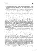
Figure 5.11 presents another perspective of the above strategy in a total
return context. As shown, return is zero for the volatility portion of this strat-
egy if yields do not move (higher or lower) from their starting point. Yet even
if the volatility portion of the strategy has a return of zero, it is possible that
the coupon income (and the income from reinvesting the coupon cash flows)
from the two-year Treasury will generate a positive overall return. Return
Risk Management 193
Price level
Changes in yield
Yields higherYields lower
This gap represents the
difference between
duration alone and
duration plus convexity;
the strategy is
increasingly profitable

as the market moves
appreciably higher or
lower beyond its
starting point.
Starting point, and point of intersection
between spot and forward positions; also
corresponds to zero change in respective
yields
Price profile for a spot 2-year Treasury
Price profile for a 3-month Treasury bill
21 months forward and leveraged seven times
FIGURE 5.10 A convexity strategy.
05_200306_CH05/Beaumont 8/15/03 12:52 PM Page 193
TLFeBOOK
can be positive when yields move appreciably from their starting point. If
all else is not equal, returns easily can turn negative if the correlation is not
a strong one between the spot yield on the two-year Treasury and the for-
ward yield on the Treasury bill position. The yields might move in opposite
directions, thus creating a situation where there is a loss from each leg of
the overall strategy. As time passes, the convexity value of the two-year
Treasury will shrink and the curvilinear profile will give way to the more
linear profile of the nonconvex futures contracts. Further, as time passes,
both lines will rotate counterclockwise into a flatter profile as consistent with
having less and less of price sensitivity to changes in yield levels.
Finally, while R and T (and sometimes Y
c
) are the two variables that dis-
tinguish spot from forward, there is not a great deal we can do about time;
time is simply going to decay one day at a time. However, R is more com-
plicated and deserves further comment.

It is a small miracle that R has not developed some kind of personality
disorder. Within finance theory, R is varyingly referred to as a risk-free rate
and a financing rate, and this text certainly alternates between both char-
acterizations. The idea behind referring to it as a risk-free rate is to highlight
that there is always an alternative investment vehicle. For example, the price
for a forward purchase of gold requires consideration of both gold’s spot
value and cost-of-carry. Although not mentioned explicitly in Chapter 2,
cost-of-carry can be thought of as an opportunity cost. It is a cost that the
purchaser of a forward agreement must pay to the seller. The rationale for
the cost is this: The forward seller of gold is agreeing not to be paid for the
194 FINANCIAL ENGINEERING, RISK MANAGEMENT, AND MARKET ENVIRONMENT
Total return
Changes in yield
O
Yields higher Yields lower
+
–
0
This dip below zero (consistent with a slight
negative return) represents transactions costs
in the event that the market does not move
dramatically one way or the other.
FIGURE 5.11 Return profile of the “gap.”
05_200306_CH05/Beaumont 8/15/03 12:52 PM Page 194
TLFeBOOK
gold until sometime in the future. The seller’s agreement to forgo an imme-
diate receipt of cash ought to be compensated. It is. The compensation is in
the form of the cost-of-carry embedded within the forward’s formula. Again,
the formula is F ϭ S (1 ϩ RT) ϭ S ϩ SRT, where SRT is cost-of-carry.
Accordingly, SRT represents the dollar (or other currency) amount that the

gold seller could have earned in a risk-free investment if he had received cash
immediately, that is, if there were an immediate settlement rather than a for-
ward settlement. R represents the risk-free rate he could have earned by
investing the cash in something like a Treasury bill. Why a Treasury bill?
Well, it is pretty much risk free. As a single cash flow security, it does not
have reinvestment risk, it does not have credit risk, and if it is held to matu-
rity, it does not pose any great price risks.
Why does R have to be risk free? Why can R not have some risk in it?
Why could SRT not be an amount earned on a short-term instrument that
has a single-A credit rating instead of the triple-A rating associated with
Treasury instruments? The simplest answer is that we do not want to con-
fuse the risks embedded within the underlying spot (e.g., an ounce of gold)
with the risks associated with the underlying spot’s cost-of-carry. In other
words, within a forward transaction, cost-of-carry should be a sideshow to
the main event. The best way to accomplish this is to reserve the cost-of-
carry component for as risk free an investment vehicle as possible.
Why is R also referred to as a financing rate? Recall the discussion of the
mechanics behind securities lending in Chapter 4. With such strategies (inclu-
sive of repurchase agreements and reverse repos), securities are lent and bor-
rowed at rates determined by the forces of supply and demand in their
respective markets. Accordingly, these rates are financing rates. Moreover, they
often are preferable to Treasury securities since the terms of securities lending
strategies can be tailor-made to whatever the parties involved desire. If the
desired trading horizon is precisely 26 days, then the agreement is structured
to last 26 days and there is no need to find a Treasury bill with exactly 26
days to maturity. Are these types of financing rates also risk free? The mar-
ketplace generally regards them as such since these transactions are collater-
alized (supported) by actual securities. Refer again to Chapter 4 for a refresher.
Let us now peel away a few more layers to the R onion. When a financ-
ing strategy is used as with securities lending or repurchase agreements, the

term of financing is obviously of interest. Sometimes an investor knows
exactly how long the financing is for, and sometimes it is ambiguous. Open
financing means that the financing will continue to be rolled over on a daily
basis until the investor closes the trade. Accordingly, it is possible that each
day’s value for R will be different from the previous day’s value. Term financ-
ing means that financing is for a set period of time (and may or may not be
rolled over). In this case, R’s value is set at the time of trade and remains
constant over the agreed-on period of time. In some instances, an investor
Risk Management 195
05_200306_CH05/Beaumont 8/15/03 12:52 PM Page 195
TLFeBOOK
who knows that a strategy is for a fixed period of time may elect to leave
the financing open rather than commit to a single term rate. Why? The
investor may believe that the benefit of a daily compounding of interest from
an open financing will be superior to a single term rate.
In the repurchase market, there is a benchmark financing rate referred
to as general collateral (GC). General collateral is the financing rate that
applies to most Treasuries at any one point in time when a forward compo-
nent of a trade comes into play. It is relevant for most off-the-run Treasuries,
but it may not be most relevant for on-the-run Treasuries. On-the-run
Treasuries tend to be traded more aggressively than off-the-run issues, and
they are the most recent securities to come to market. One implication of
this can be that they can be financed at rates appreciably lower than GC.
When this happens, whether the issue is on-the-run or off-the-run, it is said
to be on special, (or simply special). The issue is in such strong demand that
investors are willing to lend cash at an extremely low rate of interest in
exchange for a loan of the special security. As we saw, this low rate of inter-
est on the cash portion of this exchange means that the investor being lent
the cash can invest it in a higher-yielding risk-free security, such as a
Treasury bill (and pocket the difference between the two rates).

Parenthetically, it is entirely possible to price a forward on a forward
basis and price an option on a forward basis. For example, investors might
be interested in purchasing a one-year forward contract on a five-year
Treasury; however, they might not be interested in making that purchase
today; they may not want the one-year forward contract until three months
from now. Thus a forward-forward arrangement can be made. Similarly,
investors might be interested in purchasing a six-month option on a five-year
Treasury, but may not want the option to start until three months from now.
Thus, a forward-option arrangement may be made. In sum, once one under-
stands the principles underlying the triangles, any number of combinations
and permutations can be considered.
196 FINANCIAL ENGINEERING, RISK MANAGEMENT, AND MARKET ENVIRONMENT
Quantifying
risk
Options
As explained in Chapter 2, there are five variables typically required to solve
for an option’s value: price of the underlying security, the risk-free rate, time
05_200306_CH05/Beaumont 8/15/03 12:52 PM Page 196
TLFeBOOK
to expiration, volatility, and the strike price. Except for strike price (since it
typically does not vary), each of these variables has a risk measure associ-
ated with it. These risk measures are referred to as delta, rho, theta, and vega
(sometimes collectively referred to as the Greeks), corresponding to changes
in the price of the underlying, the risk-free rate, time to expiration, and
volatility, respectively. Here we discuss these measures.
Chapter 4 introduced delta and rho as option-related variables that can
be used for creating a strategy to capture and isolate changes in volatility.
Delta and rho are also very helpful tools for understanding an option’s price
volatility. By slicing up the respective risks of an option into various cate-
gories, it is possible to better appreciate why an option behaves the way it

does.
Again an option’s five fundamental components are spot, time, risk-free
rate, strike price, and volatility. Let us now examine each of these in the con-
text of risk parameters.
From a risk management perspective, how the value of a financial vari-
able changes in response to market dynamics is of great interest. For exam-
ple, we know that the measure of an option’s exposure to changes in spot
is captured by delta and that changes in the risk-free rate are captured by
rho. To complete the list, changes in time are captured by theta, and vega
captures changes in volatility. Again, the value of a call option prior to expi-
ration may be written as O
c
ϭ S(1 ϩ RT) Ϫ K ϩ V. There is no risk para-
meter associated with K since it remains constant over the life of the option.
Since every term shown has a positive value associated with it, any increase
in S, R, or V (noting that T can only shrink in value once the option is pur-
chased) is thus associated with an increase in O
c
.
For a put option, O
p
ϭ K Ϫ S(1 ϩ RT) ϩV, so now it is only a posi-
tive change in V that can increase the value of O
p
.
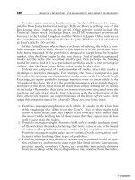
To see more precisely how delta, theta, and vega evolve in relation to
their underlying risk variable, consider Figure 5.12.
As shown in Figure 5.12, appreciating the dynamics of option risk-
characteristics can greatly facilitate understanding of strategy development.
We complete this section on option risk dynamics with a pictorial of gamma

risk (also known as convexity risk), which many option professionals view
as being equally important to delta and vega and more important that theta
or rho (see Figure 5.13).
The previous chapter discussed how these risks can be hedged for main-
stream options. Before leaving this section let’s discuss options embedded
within products. Options can be embedded within products as with callable
bonds and convertibles. By virtue of these options being embedded, they can-
not be detached and traded separately. However, just because they cannot
be detached does not mean that they cannot be hedged.
Risk Management 197
05_200306_CH05/Beaumont 8/15/03 12:52 PM Page 197
TLFeBOOK
198 FINANCIAL ENGINEERING, RISK MANAGEMENT, AND MARKET ENVIRONMENT
Delta of call
Theta of call Theta of call
K
K
K
Stock price
Vega
Delta of callDelta of put
Theta
Vega
Delta
At-the-money
Out-of-the-money
Time to expiration
In-the-money
1.0
0 –1.0

0
0
In-the-money
At-the-money
Out-of-the-money
Time to expiration
Stock price
Stock price
Stock price
FIGURE 5.12 Price sensitivities of delta, theta, and vega.
05_200306_CH05/Beaumont 8/15/03 12:52 PM Page 198
TLFeBOOK
Remember that the price of a callable bond can be defined as
P
c
ϭ P
b
Ϫ O
c
,
where P
c
ϭ Price of the callable
P
b
ϭ Price of a noncallable bond
O
c
ϭ Price of the short call option embedded in the callable
Since callable bonds traditionally come with a lockout period, the

option is in fact a deferred option or forward option. That is, the option
does not become exercisable until some time has passed after initial trading.
As an independent market exists for purchasing forward-dated options, it
is entirely possible to purchase a forward option and cancel out the effect
of a short option in a given callable. That market is the swaps market, and
the purchase of a forward-dated option gives us
P
c
ϭ P
b
Ϫ O
c
ϩ O
c
ϭ P
b
While investors do not often go through the various machinations of
purchasing a callable along with a forward-dated call option to create a syn-
thetic noncallable security, sometimes they go through the exercise on paper
Risk Management 199
At-the-money
In-the-money
Out-of-the-money
Time to maturity
Gamma
FIGURE 5.13 Gamma’s relation to time for various price and strike combinations.
05_200306_CH05/Beaumont 8/15/03 12:52 PM Page 199
TLFeBOOK
to help determine if a given callable is priced fairly in the market. They sim-
ply compare the synthetic bullet bond in price and credit terms with a true

bullet bond.
As a final comment on callables and risk management, consider the rela-
tionship between OAS and volatility. We already know that an increase in
volatility has the effect of increasing an option’s value. In the case of a
callable, a larger value of ϪO
c
translates into a smaller value for P
c
. A smaller
value for P
c
presumably means a higher yield for P
c,
given the inverse rela-
tionship between price and yield. However, when a higher (lower) volatility
assumption is used with an OAS pricing model, a narrower (wider) OAS
value results. When many investors hear this for the first time, they do a dou-
ble take. After all, if an increase in volatility makes an option’s price
increase, why doesn’t a callable bond’s option-adjusted spread (as a yield-
based measure) increase in tandem with the callable bond’s decrease in price?
The answer is found within the question. As a callable bond’s price decreases,
it is less likely to be called away (assigned maturity prior to the final stated
maturity date) by the issuer since the callable is trading farther away from
being in-the-money. Since the strike price of most callables is par (where the
issuer has the incentive to call away the security when it trades above par,
and to let the issue simply continue to trade when it is at prices below par),
anything that has the effect of pulling the callable away from being in-the-
money (as with a larger value of ϪO
c
) also has the effect of reducing the

call risk. Thus, OAS narrows as volatility rises.
200 FINANCIAL ENGINEERING, RISK MANAGEMENT, AND MARKET ENVIRONMENT
Quantifying
risk
Credit
Borrowing from the drift and default matrices first presented in Chapter 3,
a credit cone (showing hypothetical boundaries of upper and lower levels of
potential credit exposures) might be created that would look something like
that shown in Figure 5.14.
This type of presentation provides a very high-level overview of credit
dynamics and may not be as meaningful as a more detailed analysis. For
example, we may be interested to know if there are different forward-looking
total return characteristics of a single-B company that:
05_200306_CH05/Beaumont 8/15/03 12:52 PM Page 200
TLFeBOOK
Ⅲ Just started business the year before, and as a single-B company, or
Ⅲ Has been in business many years as a double-B company and was just
recently downgraded to a single-B (a fallen angel), or
Ⅲ Has been in business many years as a single-C company and was just
recently upgraded to a single-B.
In sum, not all single-B companies arrive at single-B by virtue of hav-
ing taken identical paths, and for this reason alone it should not be surprising
that their actual market performance typically is differentiated.
For example, although we might think that a single-B fallen angel is
more likely either to be upgraded after a period of time or at least to stay
at its new lower notch for some time (especially as company management
redoubles efforts to get things back on a good track), in fact the odds are
less favorable for a single-B fallen angel to improve a year after a downgrade
than a single-B company that was upgraded to a single-B status. However,
the story often is different for time horizons beyond one year. For periods

beyond one year, many single-B fallen angels successfully reposition them-
selves to become higher-rated companies. Again, the statistics available from
the rating agencies makes this type of analysis possible.
There is another dimension to using credit-related statistical experience.
Just as not all single-B companies are created in the same way, neither are
all single-B products. A single-A rated company may issue debt that is rated
double-B because it is a subordinated structure, just as a single-B rated com-
pany may issue debt that is rated double-B because it is a senior structure.
Generally speaking, for a particular credit rating, senior structures of lower-
Risk Management 201
25
20
15
10
5
0
Single C
Single B
Initial credit ratings
Likelihood of default
at end of one year (%)
FIGURE 5.14 Credit cones for a generic single-B and single-C security.
05_200306_CH05/Beaumont 8/15/03 12:52 PM Page 201
TLFeBOOK
rated companies do not fare as well as junior structures of higher-rated com-
panies. In this context, “structure” refers to the priority of cash flows that
are involved. The pattern of cash flows may be identical for both a senior
and junior bond (with semiannual coupons and a 10-year maturity), but with
very different probabilities assigned to the likelihood of actually receiving
the cash flows. The lower likelihood associated with the junior structure

means that its coupon and yield should be higher relative to a senior struc-
ture. Exactly how much higher will largely depend on investors’ expectations
of the additional cash flow risk that is being absorbed. Rating agency sta-
tistics can provide a historical or backward-looking perspective of credit risk
dynamics. Credit derivatives provide a more forward-looking picture of
credit risk expectations.
As explained in Chapter 3, a credit derivative is simply a forward, future,
or option that trades to an underlying spot credit instrument or variable.
While the pricing of the credit spread option certainly takes into consider-
ation any historical data of relevance, it also should incorporate reasonable
future expectations of the company’s credit outlook. As such, the implied
forward credit outlook can be mathematically backed-out (solved for with
relevant equations) of this particular type of credit derivative. For example,
just as an implied volatility can be derived using a standard options valua-
tion formula, an implied credit volatility can be derived in the same way
when a credit put or call is referenced and compared with a credit-free instru-
ment (as with a comparable Treasury option). Once obtained, this implied
credit outlook could be evaluated against personal sentiments or credit
agency statistics.
In 1973 Black and Scholes published a famous article (which subse-
quently was built on by Merton and others) on how to price options, called
“The Pricing of Options and Corporate Liabilities.”
6
The reference to “lia-
bilities” was to support the notion that a firm’s equity value could be viewed
as a call written on the assets of the firm, with the strike price (the point of
default) equal to the debt outstanding at expiration. Since a firm’s default
risk typically increases as the value of its assets approach the book value
(actual value in the marketplace) of the liabilities, there are three elements
that go into determining an overall default probability.

1. The market value of the firm’s assets
2. The assets’ volatility or uncertainty of value
3. The capital structure of the firm as regards the nature of its various con-
tractual obligations
202 FINANCIAL ENGINEERING, RISK MANAGEMENT, AND MARKET ENVIRONMENT
6
F. Black and M. Scholes, “The Pricing of Options and Corporate Liabilities,”
Journal of Political Economy, 81 (May–June 1973): 637–659.
05_200306_CH05/Beaumont 8/15/03 12:52 PM Page 202
TLFeBOOK
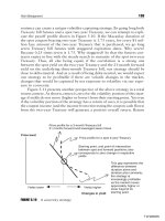
Figure 5.15 illustrates these concepts. The dominant profile resembles
that of a long call option.
Many variations of this methodology are used today, and other method-
ologies will be introduced. In many respects the understanding and quan-
tification of credit risk remains very much in its early stages of development.
Credit risk is quantified every day in the credit premiums that investors
assign to the securities they buy and sell. As these security types expand
beyond traditional spot and forward cash flows and increasingly make their
way into options and various hybrids, the price discovery process for credit
generally will improve in clarity and usefulness. Yet the marketplace should
most certainly not be the sole or final arbiter for quantifying credit risk. Aside
from more obvious considerations pertaining to the market’s own imper-
fections (occasions of unbalanced supply and demand, imperfect liquidity,
the ever-changing nature of market benchmarks, and the omnipresent pos-
sibility of asymmetrical information), the market provides a beneficial
though incomplete perspective of real and perceived risk and reward.
In sum, credit risk is most certainly a fluid risk and is clearly a consid-
eration that will be unique in definition and relevance to the investor con-
sidering it. Its relevance is one of time and place, and as such it is incumbent
on investors to weigh very carefully the role of credit risk within their over-

all approach to investing.
Risk Management 203
FIGURE 5.15 Equity as a call option on asset value.
Source: “Credit Ratings and Complementary Sources of Credit Quality Information,” Arturo
Estrella et al., Basel Committee on Banking Supervision, Bank for International Settlements,
Basel, August 2000.
05_200306_CH05/Beaumont 8/15/03 12:52 PM Page 203
[Image not available in this electronic edition.]
TLFeBOOK
This section discusses various issues pertaining to how risk is allocated in
the context of products, cash flows, and credit. By highlighting the rela-
tionships that exist across products and cash flows in particular, we see how
many investors may have a false sense of portfolio diversification because
they have failed to fully consider certain important cross-market linkages.
The very notion of allocating risk suggests that risk can somehow be
compartmentalized and then doled out on the basis of some established cri-
teria. Fair enough. Since an investor’s capital is being put to risk when invest-
ment decisions are made, it is certainly appropriate to formally establish a
set of guidelines to be followed when determining how capital is allocated.
For an individual equity investor looking to do active trading, guidelines may
consist simply of not having more than a certain amount of money invested
in one particular stock at a time and of not allowing a loss to exceed some
predetermined level. For a bond fund manager, guidelines may exist along
the lines of the individual equity investor but with added limitations per-
taining to credit risk, cash flow selection, maximum portfolio duration, and
so forth. This section is not so much directed toward how risk management
guidelines can be established (there are already many excellent texts on the
subject), but toward providing a framework for appreciating the interrelated
dynamics of the marketplace when approaching risk and decisions of how
to allocate it. To accomplish this, we present a sampling of real-world inter-

relationships for products and for cash flows.
PRODUCT INTERRELATIONSHIPS
Consider the key interrelationship between interest rates and currencies
(recalling our discussion of interest rate parity in Chapter 1) in the context
of the euro’s launch in January 1999. It can be said that prior to the melting
of 11 currencies into one, there were 11 currency volatilities melted into one.
Borrowing a concept from physics and the second law of thermodynamics—
that matter is not created or destroyed, only transformed—what happened
to those 11 nonzero volatilities that collapsed to allow for the euro’s creation?
204 FINANCIAL ENGINEERING, RISK MANAGEMENT, AND MARKET ENVIRONMENT
Allocating
risk
05_200306_CH05/Beaumont 8/15/03 12:52 PM Page 204
TLFeBOOK
One explanation might be that heightened volatility emerged among the fewer
remaining so-called global reserve currencies (namely the U.S. dollar, the yen,
and the euro), and that heightened volatility emerged among interest rates
between euro-member countries and the rest of the world. In fact, both of
these things occurred following the euro’s launch.
As a second example, consider the statistical methods between equities
and bonds presented earlier in this chapter, namely, in the discussion of how
the concepts of duration and beta can be linked with one another.
Hypothetically speaking, once a basket of particular stocks is identified that
behaves much like fixed income securities, a valid question becomes which
bundle would an investor prefer to own: a basket of synthetic fixed income
securities created with stocks or a basket of fixed income securities? The
question is deceptively simple. When investors purchase any fixed income
security, are they purchasing it because it is a fixed income security or
because it embodies the desired characteristics of a fixed income security (i.e.,
pays periodic coupons, holds capital value etc.)? If it is because they want

a fixed income security, then there is nothing more to discuss. Investors will
buy the bundle of fixed income securities. However, if they desire the char-
acteristics of a fixed income security, there is a great deal more to talk about.
Namely, if it is possible to generate fixed income returns with non–fixed
income products, why not do so? And if it is possible to outperform tradi-
tional fixed income products with non—fixed income securities and for com-
parable levels of risk, why ever buy another note or bond?
Again, if investors are constrained to hold only fixed income products,
then the choice is clear; they hold only the true fixed income portfolio. If
they want only to create a fixed income exposure to the marketplace and
are indifferent as to how this is achieved, then there are choices to make.
How can investors choose between a true and synthetic fixed income port-
folio? Perhaps on the basis of historical risk/return profiles.
If the synthetic fixed income portfolio can outperform the true fixed
income portfolio on a consistent basis at the same or a lower level of risk,
then investors might seriously want to consider owning the synthetic port-
folio. A compromise would perhaps be to own a mix of the true and syn-
thetic portfolios.
For our third example, consider the TED spread, or Treasury versus
Eurodollar spread. A common way of trading the TED spread is with futures
contracts. For example, to buy the TED spread, investors buy three-month
Treasury bill futures and sell three-month Eurodollar futures. They would
purchase the TED spread if they believed that perceptions of market risk or
volatility would increase. In short, buying the TED spread is a bet that the
spread will widen. If perceptions of increased market risk become manifest
in moves out of risky assets (namely, Eurodollar-denominated securities that
are dominated by bank issues) and into safe assets (namely, U.S. Treasury
Risk Management 205
05_200306_CH05/Beaumont 8/15/03 12:52 PM Page 205
TLFeBOOK

securities), Treasury bill yields would be expected to edge lower relative to
Eurodollar yields and the TED spread would widen. Examples of events that
might contribute to perceptions of market uncertainty would include a weak
stock market, banking sector weakness as reflected in savings and loan or
bank failures, and a national or international calamity.
Accordingly, one way for investors to create a strategy that benefits from
an expectation that equity market volatility will increase or decrease by more
than generally expected is via a purchase or sale of a fixed income spread
trade. Investors could view this as a viable alternative to delta-hedging an
equity option to isolate the value of volatility (V) within the option.
Finally, here is an example of an interrelationship between products and
credit risk. Studies have been done to demonstrate how S&P 500 futures con-
tracts can be effective as a hedge against widening credit spreads in bonds.
That is, it has been shown that over medium- to longer-run periods of time,
bond credit spreads tend to narrow when the S&P 500 is rallying, and vice
versa. Further, bond credit spreads tend to narrow when yield levels are
declining. In sum, and in general, when the equity market is in a rallying
mode, so too is the bond market. This is not altogether surprising since the
respective equity and bonds of a given company generally would be expected
to trade in line with one another; stronger when the company is doing well
and weaker when the company is not doing as well.
CASH FLOW INTERRELATIONSHIPS
Chapter 2 described the three primary cash flows: spot, forwards and
futures, and options. These three primary cash flows are interrelated by
shared variables, and one or two rather simple assumptions may be all that’s
required to change one cash flow type into another. Let us now use the tri-
angle approach to highlight these interrelationships by cash flows and their
respective payoff profiles.
A payoff profile is a simple illustration of how the return of a particu-
lar cash flow type increases or decreases as its prices rises or falls. Consider

Figure 5.16, an illustration for spot.
As shown, when the price of spot rises above its purchase price, a pos-
itive return is enjoyed. When the price of spot falls below its purchase price,
there is a loss.
Figure 5.17 shows the payoff profile for a forward or future. As read-
ers will notice, the profile looks very much like the profile for spot. It
should. Since cost-of-carry is what separates spot from forwards and
futures, the distance between the spot profile (replicated from Figure 5.16
and shown as a dashed line) and the forward/future profile is SRT (for a
non
—
cash-flow paying security). As time passes and T approaches a value
206 FINANCIAL ENGINEERING, RISK MANAGEMENT, AND MARKET ENVIRONMENT
05_200306_CH05/Beaumont 8/15/03 12:52 PM Page 206
TLFeBOOK
of zero, the forward/future profile gradually converges toward the spot pro-
file and actually becomes the spot profile. As drawn it is assumed that R
remains constant. However, if R should grow larger, the forward/future pro-
file may edge slightly to the right, and vice versa if R should grow smaller (at
least up until the forward/future expires and completely converges to spot).
Risk Management 207
0
O
Price
Return
Positive
returns
Negative
returns
Price at time of

purchase
FIGURE 5.16 Payoff profile.
0O
O
Price
Return
Positive
returns
Negative
returns
Profile for forward/future
Forward price at time of initial trade
Spot price at
time of initial trade
Profile for spot
Equal to
SRT.
Convergence between
forward/future profile
and spot profile will
occur as time passes.
FIGURE 5.17 Payoff profile for a forward or future.
05_200306_CH05/Beaumont 8/15/03 12:52 PM Page 207
TLFeBOOK
Figure 5.18 shows the payoff profile for a call option. The earlier pro-
file for spot is shown in a light dashed line and the same previous profile
for a forward/future is shown in a dark dashed line. Observe how the label
of “Price” on the x-axis has been changed to “Difference between forward
price and strike price” (or F Ϫ K). An increasingly positive difference
between F and K represents a larger in-the-money value for the option and

the return grows larger. Conversely, if the difference between F and K
remains constant or falls below zero (meaning that the price of the under-
lying security has fallen), then there is a negative return that at worst is lim-
ited to the price paid for the option. As drawn, it is assumed that R and V
remain constant. However, if R or V should grow larger, the option profile
may edge slightly to the right and vice versa if R or V should grow smaller
(at least up until the option expires and completely converges to spot).
A put payoff profile is shown in Figure 5.19. The lines are consistent
with the particular cash flows identified above.
With the benefit of these payoff profiles, let us now consider how com-
bining cash flows can create new cash flow profiles. For example, let’s cre-
ate a forward agreement payoff profile using options. As shown in Figure 5.20,
when we combine a short at-the-money put and a long at-the-money call
option, we generate the same return profile as a forward or future.
Parenthetically, a putable bond has a payoff profile of a long call
option, as it is a combination of being long a bullet (noncallable) bond and
208 FINANCIAL ENGINEERING, RISK MANAGEMENT, AND MARKET ENVIRONMENT
0
O
Return
Positive
returns
Negative
returns
Profile for
forward/future
Inflection point where
F
=
K

Profile for spot
Difference between
forward price and
strike price
Distance is
equal to
SRT
Distance is equal to
value of volatility
Price of option at
time of initial trade
FIGURE 5.18 Call payoff profile.
05_200306_CH05/Beaumont 8/15/03 12:52 PM Page 208
TLFeBOOK
a long put option. A callable bond has a payoff profile of a short put option
as it is a combination of being long a bullet bond and a short call option.
Since a putable and a callable are both ways for an investor to benefit from
steady or rising interest rates, it is unusual for investors to have both puta-
bles and callables in a single portfolio. Accordingly, it is important to rec-
ognize that certain pairings of callables and putables can result in a new cash
flow profile that is comparable to a long forward/future.
Let us now look at a combination of a long spot position and a short for-
ward/future position. This cash flow combination ought to sound familiar
because it was first presented in Chapter 4 as a basis trade (see Figure 5.21).
Next let us consider how an active delta-hedging strategy with cash and
forwards and/or futures can be used to replicate an option’s payoff profile.
Specifically, let us consider creating a synthetic option.
Risk Management 209
0
K

–
F
Return
Positive
returns
Negative
returns
FIGURE 5.19 Put payoff profile.
+ =
Long call option Short put option Long forward/future
FIGURE 5.20 Combining cash flows.
05_200306_CH05/Beaumont 8/15/03 12:52 PM Page 209
TLFeBOOK
Why might investors choose to create a synthetic option rather than buy
or sell the real thing? One reason might be the perception that the option is
trading rich (more expensive) to its fair market value. Since volatility is a
key factor when determining an option’s value, investors may create a syn-
thetic option when they believe that the true option’s implied volatility is too
high—that is, when investors believe that the expected price dynamics of the
underlying variable are not likely to be as great as that suggested by the true
option’s implied volatility. If the realized volatility is less than that implied
by the true option, then a savings may be realized.
Thus, an advantage of creating an option with forwards and Treasury
bills is that it may result in a lower cost option. However, a disadvantage of
this strategy is that it requires constant monitoring. To see why, we need to
revisit the concept of delta.
As previously discussed, delta is a measure of an option’s exposure to
the price dynamics of the underlying security. Delta is positive for a long call
option because a call trades to a long position in the underlying security.
Delta is negative for a long put option because a put trades to a short posi-

tion in the underlying security. The absolute value of an option’s delta
becomes closer to 1 as it moves in-the-money and becomes closer to zero as
it moves out-of-the-money. An option that is at-the-money tends to have a
delta close to 0.5.
Let us say that investors desire an option with an initial delta of 0.5. If
a true option is purchased, delta will automatically adjust to price changes
in the underlying security. For example, if a call option is purchased on a
share of General Electric (GE) equity, delta will automatically move closer
to 1 as the share price rises. Conversely, delta will move closer to zero as
210 FINANCIAL ENGINEERING, RISK MANAGEMENT, AND MARKET ENVIRONMENT
+ =
Long spot Short forward/future Basis trade
The distance between
where these two payoff
profiles cross the price
line is equal to
SRT
, cost-
of-carry.
FIGURE 5.21 A basis trade.
05_200306_CH05/Beaumont 8/15/03 12:52 PM Page 210
TLFeBOOK
the share price falls. Delta of a synthetic option must be monitored constantly
because it will not automatically adjust itself to price changes in the under-
lying security.
If an initial delta of 0.5 is required for a synthetic call option, then
investors will go long a forward to cover half (0.5) of the underlying secu-
rity’s face value, and Treasury bills will be purchased to cover 100 percent
of the underlying security’s forward value. We cover 100 percent of the secu-
rity’s forward value because this serves to place a “floor” under the strat-

egy’s profit/loss profile. If yields fall and the implied value for delta increases,
a larger forward position will be required. If yields rise and the implied value
for delta decreases, a smaller forward position will be required. The more
volatile the underlying security, the more expensive it will become to man-
age the synthetic option. This is consistent with the fact that an increase in
volatility serves to increase the value of a true option. The term implied delta
means the value delta would be for a traditional option when valued using
the objective strike price and expected volatility. Just how we draw a syn-
thetic option’s profit/loss profile depends on a variety of assumptions. For
example, since the synthetic option is created with Treasury bills and for-
wards, are the Treasury bills financed in the repo market? If yes, this would
serve to lever the synthetic strategy. It is an explicit assumption of traditional
option pricing theory that the risk-free asset (the Treasury bill) is leveraged
(i.e., the Treasury bill is financed in the repo market).
Repo financing on a synthetic option that is structured with a string of
overnight repos is consistent with creating a synthetic American option,
which may be exercised at any time. Conversely, the repo financing structured
with a term repo is consistent with a European option, which may be exer-
cised only at option maturity. Since there is no secondary market for repo
transactions, and since investors may not have the interest or ability to exe-
cute an offsetting repo trade, a string of overnight repos may be the best
strategy with synthetic options.
By going long a forward, we are entering into an agreement to purchase
the underlying security at the forward price. Thus, if the actual market price
lies anywhere above (below) the forward price at the expiration of the for-
ward, then there is a profit (loss). There is a profit (loss) because we pur-
chase the underlying security at a price below (above) the prevailing market
price and in turn sell that underlying security at the higher (lower) market
price. Of course, once the underlying security is purchased, investors may
decide to hang onto the security rather than sell it immediately and realize

any gains (losses). Investors may choose to hold onto the security for a while
in hopes of improving returns.
A long option embodies the right to purchase the underlying security. This
is in contrast to a long forward (or a long future) that embodies the obliga-
tion to purchase the underlying security. Thus, an important distinction to
Risk Management 211
05_200306_CH05/Beaumont 8/15/03 12:52 PM Page 211
TLFeBOOK
be made between a true option and an option created with Treasury bills and
forwards is that the former does not commit investors to a forward purchase.
Although secondary markets (markets where securities may be bought
or sold long after they are initially launched) may not be well developed for
all types of forward transactions, an offsetting trade may be made easily if
investors want to reverse the synthetic option strategy prior to expiration.
For example, one month after entering into a three-month forward to pur-
chase a 10-year Treasury, investors may decide to reverse the trade. To do
this, investors would simply enter into a two-month forward to sell the 10-
year Treasury. In short, these forward transactions would still require
investors to buy and sell the 10-year Treasury at some future date. However,
these offsetting transactions allow investors to “close out” the trade prior
to the maturity of the original forward transaction. “Close out” appears in
quotes because the term conveys a sense of finality. Although an offsetting
trade is indeed executed for purposes of completing the strategy, the strat-
egy is not really dead until the forwards mature in two months’ time. And
when we say that an offsetting forward transaction is executed, we mean
only that an opposite trade is made on the same underlying security and for
the same face value. The forward price of an offsetting trade could be higher,
lower, or the same as the forward price of the original forward trade. The
factor that determines the price on the offsetting forward is the same factor
that determines the price on the original forward contract: cost-of-carry.

Figure 5.22 shows how combining forwards and Treasury bills creates
a synthetic option profile. The profile shown is at the expiration of the syn-
thetic option.
If the synthetic call option originally were designed to have a delta of 0.5,
then the investors would go long a forward to cover half of the underlying
security’s face value and would purchase Treasury bills equal to 100 percent
of the underlying security’s forward value. One half of the underlying security’s
face value is the benchmark for the forward position because the target delta
is 0.5. If the target delta were 0.75, then three quarters of the underlying
security’s face value would be the benchmark. If the price of the underly-
ing security were to rise (fall), then the forward position would be increased
(decreased) to increase (decrease) the implied delta. The term implied delta
means the value for delta if our synthetic option were a true option.
The preceding example assumes that the synthetic option is intended to
underwrite 100 percent of the underlying asset. For this reason our at-the-
money synthetic option requires holding 50 percent of the underlying face
value in our forward position. If our synthetic option were to move in-the-
money with delta going from 0.5 to close to 1.0, we would progressively hold
up to 100 percent of the underlying’s face value in our forward position.
212 FINANCIAL ENGINEERING, RISK MANAGEMENT, AND MARKET ENVIRONMENT
05_200306_CH05/Beaumont 8/15/03 12:52 PM Page 212
TLFeBOOK
It is a simple matter to determine the appropriate size of the forward
position for underwriting anything other than 100 percent of the underly-
ing asset. For example, let us assume that we want to underwrite 50 per-
cent of the underlying asset. In this instance, we would want to own 50
percent of the underlying’s face value in Treasury bills and 25 percent of the
underlying’s forward value for an at-the-money option. The delta for an at-
the-money option is 0.5, and 50 percent times 0.5 is equal to 25 percent.
Thus, we want to own 25 percent of the underlying’s forward value in our

forward position.
Again, the delta of a synthetic option will not adjust itself continuously
to price changes in the underlying security. Forward positions must be man-
aged actively, and the transaction costs implied by bid/offer spreads on suc-
cessive forward transactions are an important consideration. Thus, how well
the synthetic option performs relative to the true option depends greatly on
market volatility. The more transactions required to manage the synthetic
option, the greater its cost. The horizontal piece of the profit/loss profile is
drawn below zero to reflect expected cumulative transactions costs at expi-
ration. Thus, expected volatility may very well be the most important crite-
rion for investors to consider when evaluating a synthetic versus a true option
Risk Management 213
This distance below a zero total
return represents the
transaction costs associated
with the constant fine-tuning
required for a synthetic option.
In short, the floor return
(generated by the fixed and
known return on the Treasury
bill) is lowered by the costs of
delta hedging.
Synthetic option
Treasury forwardTreasury bill
Total return
Total return Total return
At maturity of the
synthetic option
At maturity of
the Treasury bill

At maturity of
the Treasury bill
FIGURE 5.22 Synthetic option profile.
05_200306_CH05/Beaumont 8/15/03 12:52 PM Page 213
TLFeBOOK
strategy. That is, if investors believe that the true option is priced rich on a
volatility basis, they may wish to create a synthetic option. If the realized
volatility happens to be less than that implied by the true option, then the
synthetic option may well have been the more appropriate vehicle for exe-
cuting the option strategy.
Finally, the nature of discrete changes in delta may pose special chal-
lenges when investors want to achieve a delta of zero. For example, there
may be a market level where investors would like to close out the synthetic
option. Since it is unlikely investors can monitor the market constantly, they
probably would leave market orders of where to buy or sell predetermined
amounts of forwards or Treasury bills. However, just leaving a market order
to be executed at a given level does not guarantee that the order will be filled
at the prices specified. In a fast-moving market, it may well be impossible
to fill a large order at the desired price. An implication is that a synthetic
option may be closed out, yet at an undesirable forward price. Accordingly,
the synthetic option may prove to be a less efficient investment vehicle than
a true option. Thus, creating synthetic options may be a worthwhile con-
sideration only when replicating option markets that are less efficient. That
is, a synthetic strategy may prove to be more successful when structured
against a specialized option-type product with a wide bid/ask spread as
opposed to replicating an exchange-traded option.
Aside from using Treasury bills and forwards to create options, Treasury
bills may be combined with Treasury note or bond futures, and Treasury bill
futures may be combined with Treasury note or bond futures and/or for-
wards. However, investors need to consider the nuances of trading in these

other products. For example, a Treasury bill future expires into a three-
month cash bill; it does not expire at par. Further, Treasury futures have
embedded delivery options.
Let us now take a step back for a moment and consider what has been
presented thus far. Individual investors are capable of knowing the products
and cash flows in their portfolio at any point in time. However, at the com-
pany level of investing (as with a large institutional fund management com-
pany or even an investment bank), it would be unusual for any single trader
to have full knowledge of the products and cash flows held by other traders.
Generally speaking, only the high-level managers of firms have full access
to individual trading records. Something that clearly is of interest to high-
level managers is how the firm’s risk profile appears on an aggregated basis
as well as on a trader-by-trader basis. In other words, assume for a moment
that there is just one single firm-wide portfolio that is composed of dozens
(or even hundreds) of individual portfolios. What would be the risk profile
of that single firm-wide portfolio? In point of fact, it may not be as large as
you might think. Why not? Because every portfolio manager may not be fol-
lowing the same trading strategies as everyone else, and/or the various strate-
214 FINANCIAL ENGINEERING, RISK MANAGEMENT, AND MARKET ENVIRONMENT
05_200306_CH05/Beaumont 8/15/03 12:52 PM Page 214
TLFeBOOK
gies may be constructed with varying cash flows. Let us consider an exam-
ple involving multiple traders, where each trader is limited to having one
strategy in the portfolio at any given time.
Say that trader A has a volatility trade in her portfolio that was created
by going long an at-the-money call option and an at-the-money put option.
Trader A simply believes that volatility is going to increase more than gen-
erally expected. Say trader B has a future in his portfolio and believes that
the underlying security will appreciate in price. Note that these trades may
not at all appear to be contradictory on the surface. Volatility can increase

even without a change in pattern of the underlying asset’s price (as with a
surprise announcement affecting all stocks, such as the sudden news that the
federal government will shut down over an indefinite period owing to a dead-
lock with the Congress over certain key budget negotiations). Such a risk
type is sometime referred to as event risk. The whole idea behind isolating
volatility is to be indifferent to such asset price moves. From the presenta-
tions above, we know that a future can be created with a long at-the-money
call option and a short at-the-money put option. Accordingly, when we sum
across the portfolios of traders A and B we have
O
c
ϩ O
p
ϩ O
c
Ϫ O
p
ϭ 2 ϫ O
c
.
By combining one strategy that is indifferent to price moves with
another that expects higher prices, the net effect is a strong bias to upward-
moving prices. It should now be easy to appreciate how an aggregation of
individual strategies can be a necessary and insightful exercise for firms with
large trading operations.
Let us now take this entire discussion a step further. Assume that all of
a firm’s cash flows have been distilled into one of three categories: spot, for-
ward and futures, and options. The aggregate spot position may reflect a
net positive outlook for market prices; the net forward and future position
also may reflect a net positive outlook though on a smaller scale; and the

net option position may reflect a negative outlook on volatility. Could all of
these net cash flows be melted into a single dollar (or other currency) value?
Yes, if we can be permitted to make some assumptions to simplify the issue.
For example, we already know from our various tours around the triangle
that with some pretty basic assumptions, we can bring a forward /future or
option back to spot. By doing this we could distill an entire firm’s trading
operation into a single number. Would such a number have limitations to
meaningful interpretation? Absolutely yes. The fact that we could distill myr-
iad products and cash flows into a single value does not mean that we can
or should rely on it as a daily gauge of capital at risk. We can think of quan-
tifying risk as an exercise that can fall along a continuum. At one end of the
Risk Management 215
05_200306_CH05/Beaumont 8/15/03 12:52 PM Page 215
TLFeBOOK
continuum we can let each strategy stand on its own as an individual trans-
action, and at the other end of the continuum we have the ability (though
only with some strong assumptions) to reduce a complex network of strate-
gies into a single value. What one firm will find most relevant and mean-
ingful may not be the same as any other firm, and the optimal risk
management profiles and methodologies may well come only with perse-
verance, creativity, and trial and error.
Credit Interrelationships
As discussed in some detail in Chapter 3, credit permeates all aspects of
finance. Credit risk always will exist in its own right, and while it can take
on a rather explicit shape in the form of different market products, it also
can be transformed by an issuer’s particular choice of cash flows. The deci-
sion of how far investors ought to extend their credit risk exposure is fun-
damental. All investors have some amount of capital in support of their
trading activity, and a clear objective ought to be the continuous preserva-
tion of at least some portion of that capital so that the portfolio can live to

invest another day. While investments with greater credit risks often provide
greater returns as compensation for that added risk, riskier investments also
can mean poor performance. Thus, it is essential for all investors to have
clear guidelines for just how much credit risk is acceptable and in all of its
forms.
Figure 5.23 provides a snapshot of some of the considerations that larger
investors may want to include in a methodology for allocating credit risk.
Generally speaking, a large firm will place ceilings or upper limits on the
216 FINANCIAL ENGINEERING, RISK MANAGEMENT, AND MARKET ENVIRONMENT
Part of the world
Country
Industry
Company
Investment product type
Asia ($5 billion)
Japan ($2 billion)
Automotives ($0.5 billion)
Nissan ($0.1 billion)
Nissan equity ($0.04 billion)
Assume a total of $20 billion in a firm's capital to be allocated globally
FIGURE 5.23 Allocating risk capital.
05_200306_CH05/Beaumont 8/15/03 12:52 PM Page 216
TLFeBOOK
amount of investment funds that can be allocated to any one category, where
category might be a part of the world, a particular country, or a specific com-
pany. While the map might be excessive for some investors, it could be woe-
fully incomplete for others. For example, GE is a large company. Does the
credit officer of a large bank limit investments to GE businesses with GE
taken as a whole, or does she recognize that GE is made up of many diver-
sified businesses that deserve to be given separate industry-specific risk allo-

cations? Perhaps she creates a combination of the two different approaches
and evaluates situations on more of a case-by-case basis.
As shown in Figure 5.22, the first layer of a top/down capital allocation
process may be by “part of the world,” followed by “country,” and so on.
At each successive step lower, the amount of capital available diminishes.
Since Japan is not the only country in Asia, and since a company is unlikely
to put all of its Asian-designated capital into just Japan, the amount of cap-
ital allocated to Japan will be something less than the amount of capital allo-
cated to Asia generally. Similarly, since automotives is not the only industry
in Japan, the amount of capital allocated to automotives will be something
less than the amount of capital allocated to Japan, and so on.
Clearly, the credit risk allocation methodology that is ultimately selected
by any investor will be greatly dependent on investment objectives, capital
base, and financial resources. While there is no single right way of doing it,
just as there is no single right way of investing, at least there are well-rec-
ognized quantitative and qualitative measures of credit risk that can be tai-
lored to appropriate and meaningful applications.
Summary
In this section, we have discussed the interrelationships of risk in the con-
text of products, cash flows, and credit. We now conclude with a discussion
of ways that a firm’s capital can be allocated to different business lines that
involve the taking of various risks. Since capital guidelines and restrictions
are also a way that certain financial companies are regulated (as with insur-
ance firms and banks), we further explore the topic of capital allocation in
Chapter 6.
Generally speaking, risk limits are expressed as ceilings—upper limits
on how much capital may be committed to a particular venture (as with secu-
rities investments, the making of loans, the basic running of a particular busi-
ness operation, etc.). For especially large companies, ceilings might exist for
how much capital might be committed to a particular country or part of the

world. For smaller investment companies, ceilings might exist simply for how
much capital might be allocated to different types of securities.
Risk Management 217
05_200306_CH05/Beaumont 8/15/03 12:52 PM Page 217
TLFeBOOK