Introduction to Algorithms Second Edition Instructor’s Manual 2nd phần 6 pps
Bạn đang xem bản rút gọn của tài liệu. Xem và tải ngay bản đầy đủ của tài liệu tại đây (289.32 KB, 43 trang )
14-8 Lecture Notes for Chapter 14: Augmenting Data Structures
If search goes left:
•
If there is an overlap in left subtree, done.
•
If there is no overlap in left, show there is no overlap in right.
•
Went left because:
low[i] ≤ max[left[x]]
= high[ j] for some j in left subtree .
•
Since there is no overlap in left, i and j don’t overlap.
•
Refer back to: no overlap if
low[i] > high[ j ]or low[ j] > high[i] .
•
Since low[i] ≤ high[ j ], must have low[ j] > high[i].
•
Now consider any interval k in right subtree.
•
Because keys are low endpoint,
low[ j ]
in left
≤ low[k]
in right
.
•
Therefore, high[i] < low[ j] ≤ low[k].
•
Therefore, high[i] < low[k].
•
Therefore, i and k do not overlap. (theorem)
Solutions for Chapter 14:
Augmenting Data Structures
Solution to Exercise 14.1-5
Given an element x in an n-node order-statistic tree T and a natural number i, the
following procedure retrieves the ith successor of x in the linear order of T :
OS-S
UCCESSOR(T, x, i)
r ← OS-R
ANK(T, x)
s ← r +i
return OS-S
ELECT(root[T ], s)
Since OS-R
ANK and OS-SELECT each take O(lg n) time, so does the procedure
OS-SUCCESSOR.
Solution to Exercise 14.1-6
When inserting node z, we search down the tree for the proper place for z. For each
node x on this path, add 1 to rank[x]ify is inserted within x’s left subtree, and
leave rank[x] unchanged if y is inserted within x’s right subtree. Similarly when
deleting, subtract 1 from rank[x] whenever the spliced-out node y had been in x’s
left subtree.
We also need to handle the rotations that occur during the Þxup procedures for
insertion and deletion. Consider a left rotation on node x, where the pre-rotation
right child of x is y (so that x becomes y’s left child after the left rotation). We
leave rank[x] unchanged, and letting r = rank[y] before the rotation, we set
rank[y] ← r + rank[x]. Right rotations are handled in an analogous manner.
Solution to Exercise 14.1-7
Let A[1 n] be the array of n distinct numbers.
One way to count the inversions is to add up, for each element, the number of larger
elements that precede it in the array:
14-10 Solutions for Chapter 14: Augmenting Data Structures
# of inversions =
n
j=1
|
Inv( j )
|
,
where Inv( j) =
{
i : i < j and A[i] > A[ j]
}
.
Note that
|
Inv( j )
|
is related to A[ j]’s rank in the subarray A[1 j ] because the
elements in Inv( j) are the reason that A[ j ] is not positioned according to its rank.
Let r ( j ) be the rank of A[ j ]inA[1 j ]. Then j = r ( j) +
|
Inv( j )
|
,sowecan
compute
|
Inv( j )
|
= j −r( j )
by inserting A[1], ,A[n] into an order-statistic tree and using OS-RANK to Þnd
the rank of each A[ j] in the tree immediately after it is inserted into the tree. (This
OS-R
ANK value is r( j ).)
Insertion and OS-R
ANK each take O(lg n) time, and so the total time for n ele-
ments is O(n lg n).
Solution to Exercise 14.2-2
Yes, by Theorem 14.1, because the black-height of a node can be computed from
the information at the node and its two children. Actually, the black-height can
be computed from just one child’s information: the black-height of a node is the
black-height of a red child, or the black height of a black child plus one. The
second child does not need to be checked because of property 5 of red-black trees.
Within the RB-I
NSERT-FIXUP and RB-DELETE-FIXUP procedures are color
changes, each of which potentially cause O(lg n) black-height changes. Let us
show that the color changes of the Þxup procedures cause only local black-height
changes and thus are constant-time operations. Assume that the black-height of
each node x is kept in the Þeld bh[x].
For RB-I
NSERT-FIXUP, there are 3 cases to examine.
Case 1: z’s uncle is red.
C
DA
B
α
βγ
δε
(a)
C
DA
B
α
βγ
δε
C
DB
δε
C
D
B
A
αβ
γδε
(b)
A
αβ
γ
k+1
k+1
k+1
k+1 k+1
k+2
k+1
k+1
k+1
k+1
k+1
k+1
k+1
k+1
k+2
k+1z
y
z
y
Solutions for Chapter 14: Augmenting Data Structures 14-11
•
Before color changes, suppose that all subtrees α, β, γ , δ, have the same
black-height k with a black root, so that nodes A, B, C, and D have black-
heights of k + 1.
•
After color changes, the only node whose black-height changed is node C.
To Þx that, add bh[ p[ p[z]]] = bh[p[p[z]]] + 1 after line 7 in RB-INSERT-
F
IXUP.
•
Since the number of black nodes between p[ p[z]] and z remains the same,
nodes above p[p[z]] are not affected by the color change.
Case 2: z’s uncle y is black, and z is a right child.
Case 3: z
’s uncle y is black, and z is a left child.
C
A
B
α
βγ
δ
Case 2
B
A
αβ
γ
δ
Case 3
A
B
C
αβ γδ
C
k+1
k+1
k+1 k+1
k+1
k+1
k+1 k+1
k+1
z
y
z
y
•
With subtrees α, β, γ , δ, of black-height k, we see that even with color
changes and rotations, the black-heights of nodes A, B, and C remain the
same (k + 1).
Thus, RB-I
NSERT-FIXUP maintains its original O(lg n) time.
For RB-D
ELETE-FIXUP, there are 4 cases to examine.
Case 1: x’s sibling w is red.
A
B
D
CE
αβ
γδεζ
xw
A
B
C
D
E
x new w
αβγ δ
εζ
Case 1
•
Even though case 1 changes colors of nodes and does a rotation, black-
heights are not changed.
•
Case 1 changes the structure of the tree, but waits for cases 2, 3, and 4 to
deal with the “extra black” on x.
Case 2: x’s sibling w is black, and both of w’s children are black.
A
B
D
CE
αβ
γδεζ
xw
c
A
B
D
CE
αβ
γδεζ
cnew x
Case 2
14-12 Solutions for Chapter 14: Augmenting Data Structures
•
w is colored red, and x’s “extra” black is moved up to p[x].
•
Now we can add bh[p[x]] = bh[x] after line 10 in RB-DELETE-FIXUP.
•
This is a constant-time update. Then, keep looping to deal with the extra
black on p[x].
Case 3: x’s sibling w is black, w’s left child is red, and w’s right child is black.
A
B
D
C E
αβ
γδεζ
xw
c
A
B
C
D
αβ γ
δ
εζ
x
c
new w
Case 3
E
•
Regardless of the color changes and rotation of this case, the black-heights
don’t change.
•
Case 3 just sets up the structure of the tree, so it can fall correctly into case 4.
Case 4: x’s sibling w is black, and w’s right child is red.
A
B
D
CE
αβ
γδ
εζ
xw
c c
αβ
A
B
C
D
E
new x = root[T]
γδεζ
Case 4
c′ c′
•
Nodes A, C, and E keep the same subtrees, so their black-heights don’t
change.
•
Add these two constant-time assignments in RB-DELETE-FIXUP after
line 20:
bh[ p[x]] = bh[x] + 1.
bh[ p[ p[x]]] = bh[ p[x]] +1.
•
The extra black is taken care of. Loop terminates.
Thus, RB-D
ELETE-FIXUP maintains its original O(lg n) time.
Therefore, we conclude that black-heights of nodes can be maintained as Þelds
in red-black trees without affecting the asymptotic performance of red-black tree
operations.
Solution to Exercise 14.2-3
No, because the depth of a node depends on the depth of its parent. When the depth
of a node changes, the depths of all nodes below it in the tree must be updated.
Updating the root node causes n −1 other nodes to be updated, which would mean
that operations on the tree that change node depths might not run in O(n lg n) time.
Solutions for Chapter 14: Augmenting Data Structures 14-13
Solution to Exercise 14.3-3
As it travels down the tree, INTERVAL-SEARCH Þrst checks whether current node x
overlaps the query interval i and, if it does not, goes down to either the left or right
child. If node x overlaps i , and some node in the right subtree overlaps i ,but
no node in the left subtree overlaps i , then because the keys are low endpoints,
this order of checking (Þrst x, then one child) will return the overlapping interval
with the minimum low endpoint. On the other hand, if there is an interval that
overlaps i in the left subtree of x, then checking x before the left subtree might
cause the procedure to return an interval whose low endpoint is not the minimum
of those that overlap i. Therefore, if there is a possibility that the left subtree might
contain an interval that overlaps i, we need to check the left subtree Þrst. If there is
no overlap in the left subtree but node x overlaps i, then we return x. We check the
right subtree under the same conditions as in I
NTERVAL-SEARCH: the left subtree
cannot contain an interval that overlaps i, and node x does not overlap i, either.
Because we might search the left subtree Þrst, it is easier to write the pseudocode to
use a recursive procedure M
IN-INTERVAL-SEARCH-FROM(T, x, i), which returns
the node overlapping i with the minimum low endpoint in the subtree rooted at x,
or nil[T ] if there is no such node.
M
IN-INTERVAL-SEARCH(T, i)
return M
IN-INTERVAL-SEARCH-FROM(T, root[T ], i)
M
IN-INTERVAL-SEARCH-FROM(T, x, i)
if left[x] = nil[T ] and max[left[x]] ≥ low[i]
then y ← M
IN-INTERVAL-SEARCH-FROM(T, left[x], i)
if y = nil[T ]
then return y
elseif i overlaps int[x]
then return x
else return nil[T ]
elseif i overlaps int[x]
then return x
else return M
IN-INTERVAL-SEARCH-FROM(T, right[x], i)
The call M
IN-INTERVAL-SEARCH(T, i) takes O(lg n) time, since each recursive
call of MIN-INTERVAL-SEARCH-FROM goes one node lower in the tree, and the
height of the tree is O(lg n).
Solution to Exercise 14.3-6
1. Underlying data structure:
A red-black tree in which the numbers in the set are stored simply as the keys
of the nodes.
14-14 Solutions for Chapter 14: Augmenting Data Structures
SEARCH is then just the ordinary TREE-SEARCH for binary search trees, which
runs in O(lg n) time on red-black trees.
2. Additional information:
The red-black tree is augmented by the following Þelds in each node x:
•
min-gap[x] contains the minimum gap in the subtree rooted at x. It has the
magnitude of the difference of the two closest numbers in the subtree rooted
at x.Ifx is a leaf (its children are all nil[T ]), let min-gap[x] =∞.
•
min-val[x] contains the minimum value (key) in the subtree rooted at x.
•
max-val[x] contains the maximum value (key) in the subtree rooted at x.
3. Maintaining the information:
The three Þelds added to the tree can each be computed from information in the
node and its children. Hence by Theorem 14.1, they can be maintained during
insertion and deletion without affecting the O(lg n) running time:
min-val[x] =
min-val[left[x]] if there’s a left subtree ,
key[x] otherwise ,
max-val[x] =
max-val[right[x]] if there’s a right subtree ,
key[x] otherwise ,
min-gap[x] = min
⎧
⎪
⎪
⎨
⎪
⎪
⎩
min-gap[left[x]] (∞ if no left subtree) ,
min-gap[right[x]] (∞ if no right subtree) ,
key[x
] − max-val[left[x]] (∞ if no left subtree) ,
min-val[right[x]] − key[x](∞ if no right subtree) .
In fact, the reason for deÞning the min-val and max-val Þelds is to make it
possible to compute min-gap from information at the node and its children.
4. New operation:
M
IN-GAP simply returns the min-gap stored at the tree root. Thus, its running
time is O(1).
Note that in addition (not asked for in the exercise), it is possible to Þnd the
two closest numbers in O(lg n) time. Starting from the root, look for where the
minimum gap (the one stored at the root) came from. At each node x, simulate
the computation of min-gap[x]toÞgure out where min-gap[x] came from. If
it came from a subtree’s min-gap Þeld, continue the search in that subtree. If
it came from a computation with x’s key, then x and that other number are the
closest numbers.
Solution to Exercise 14.3-7
General idea: Move a sweep line from left to right, while maintaining the set of
rectangles currently intersected by the line in an interval tree. The interval tree
will organize all rectangles whose x interval includes the current position of the
sweep line, and it will be based on the y intervals of the rectangles, so that any
overlapping y intervals in the interval tree correspond to overlapping rectangles.
Solutions for Chapter 14: Augmenting Data Structures 14-15
Details:
1. Sort the rectangles by their x-coordinates. (Actually, each rectangle must ap-
pear twice in the sorted list—once for its left x-coordinate and once for its right
x-coordinate.)
2. Scan the sorted list (from lowest to highest x-coordinate).
•
When an x-coordinate of a left edge is found, check whether the rectangle’s
y-coordinate interval overlaps an interval in the tree, and insert the rectangle
(keyed on its y-coordinate interval) into the tree.
•
When an x-coordinate of a right edge is found, delete the rectangle from the
interval tree.
The interval tree always contains the set of “open” rectangles intersected by the
sweep line. If an overlap is ever found in the interval tree, there are overlapping
rectangles.
Time: O(n lg n)
•
O(n lg n) to sort the rectangles (we can use merge sort or heap sort).
•
O(n lg n) for interval-tree operations (insert, delete, and check for overlap).
Solution to Problem 14-1
a. Assume for the purpose of contradiction that there is no point of maximum
overlap in an endpoint of a segment. The maximum overlap point p is in the
interior of m segments. Actually, p is in the interior of the intersection of those
m segments. Now look at one of the endpoints p
of the intersection of the m
segments. Point p
has the same overlap as p because it is in the same intersec-
tion of m segments, and so p
is also a point of maximum overlap. Moreover, p
is in the endpoint of a segment (otherwise the intersection would not end there),
which contradicts our assumption that there is no point of maximum overlap in
an endpoint of a segment. Thus, there is always a point of maximum overlap
which is an endpoint of one of the segments.
b. Keep a balanced binary tree of the endpoints. That is, to insert an interval,
we insert its endpoints separately. With each left endpoint e, associate a value
p[e] =+1 (increasing the overlap by 1). With each right endpoint e associate a
value p[e] =−1 (decreasing the overlap by 1). When multiple endpoints have
the same value, insert all the left endpoints with that value before inserting any
of the right endpoints with that value.
Here’s some intuition. Let e
1
, e
2
, , e
n
be the sorted sequence of endpoints
corresponding to our intervals. Let s(i, j) denote the sum p[e
i
] + p[e
i+1
] +
···+p[e
j
] for 1 ≤ i ≤ j ≤ n. We wish to Þnd an i maximizing s(1, i).
Each node x stores three new attributes. Suppose that the subtree rooted at x
includes the endpoints e
l[x ]
, ,e
r[x]
. We store v[x] = s(l[x], r[x]), the sum of
the values of all nodes in x’s subtree. We also store m[x], the maximum value
14-16 Solutions for Chapter 14: Augmenting Data Structures
obtained by the expression s(l[x], i) for any i in
{
l[x], l[x] + 1, ,r[x]
}
. Fi-
nally, we store o[x] as the value of i for which m[x] achieves its maximum. For
the sentinel, we deÞne v[nil[T ]] = m[nil[T ]] = 0.
We can compute these attributes in a bottom-up fashion to satisfy the require-
ments of Theorem 14.1:
v[x] = v[left[x]] + p[x] + v[right[x]] ,
m[x] = max
⎧
⎨
⎩
m[left[x
]] (max is in x’s left subtree) ,
v[left[x]] + p[x] (max is at x) ,
v[left[x]] + p[x] +m[right[x]] (max is in x’s right subtree) .
The computation of v[x] is straightforward. The computation of m[x] bears
further explanation. Recall that it is the maximum value of the sum of the
p values for the nodes in x’s subtree, starting at l[x], which is the leftmost
endpoint in x’s subtree and ending at any node i in x’s subtree. The value
of i that maximizes this sum is either a node in x’s left subtree, x itself, or
a node in x’s right subtree. If i is a node in x’s left subtree, then m[left[x]]
represents a sum starting at l[x], and hence m[x] = m[left[x]]. If i
is x itself,
then m[x] represents the sum of all p values in x’s left subtree plus p[x], so
that m[x] = v[left[x]] + p[x]. Finally, if i is in x’s right subtree, then m[x]
represents the sum of all p values in x’s left subtree, plus p[x], plus the sum
of some set of p values in x’s right subtree. Moreover, the values taken from
x’s right subtree must start from the leftmost endpoint in the right subtree. To
maximize this sum, we need to maximize the sum from the right subtree, and
that value is precisely m[right[x]]. Hence, in this case, m[x] = v[left[x]] +
p[x] + m[right[x]].
Once we understand how to compute m[x], it is straightforward to compute
o[x] from the information in x and its two children. Thus, we can implement
the operations as follows:
•
INTERVAL-INSERT: insert two nodes, one for each endpoint of the interval.
•
INTERVAL-DELETE: delete the two nodes representing the interval end-
points.
•
FIND-POM: return the interval whose endpoint is represented by o[root[T ]].
Because of how we have deÞned the new attributes, Theorem 14.1 says that
each operation runs in O(lg n) time. In fact, F
IND-POM takes only O(1) time.
Solution to Problem 14-2
a. We use a circular list in which each element has two Þelds, key and next.At
the beginning, we initialize the list to contain the keys 1, 2, ,n in that order.
This initialization takes O(n) time, since there is only a constant amount of
work per element (i.e., setting its key and its next Þelds). We make the list
circular by letting the next Þeld of the last element point to the Þrst element.
We then start scanning the list from the beginning. We output and then delete
every mth element, until the list becomes empty. The output sequence is the
Solutions for Chapter 14: Augmenting Data Structures 14-17
(n, m)-Josephus permutation. This process takes O(m) time per element, for a
total time of O(mn). Since m is a constant, we get O(mn) = O(n) time, as
required.
b. We can use an order-statistic tree, straight out of Section 14.1. Why? Suppose
that we are at a particular spot in the permutation, and let’s say that it’s the jth
largest remaining person. Suppose that there are k ≤ n people remaining. Then
we will remove person j, decrement k to reßect having removed this person,
and then go on to the ( j +m −1)th largest remaining person (subtract 1 because
we have just removed the jth largest). But that assumes that j + m ≤ k. If not,
then we use a little modular arithmetic, as shown below.
In detail, we use an order-statistic tree T , and we call the procedures OS-
I
NSERT, OS-DELETE, OS-RANK, and OS-SELECT:
J
OSEPHUS(n, m)
initialize T to be empty
for j ← 1 to n
do create a node x with key[x] = j
OS-I
NSERT(T, x)
k ← n
j ← m
while k > 2
do x ← OS-S
ELECT(root[T ], j)
print key[x]
OS-D
ELETE(T, x)
k ← k − 1
j ← (( j + m − 2) mod k) + 1
print key[OS-S
ELECT(root[T ], 1)]
The above procedure is easier to understand. Here’s a streamlined version:
J
OSEPHUS(n, m)
initialize T to be empty
for j ← 1 to n
do create a node x with key[x] = j
OS-I
NSERT(T, x)
j ← 1
for k ← n downto 1
do j ← (( j + m − 2) mod k) + 1
x ← OS-S
ELECT(root[T ], j)
print key[x]
OS-D
ELETE(T, x)
Either way, it takes O(n lg n) time to build up the order-statistic tree T , and
then we make O(n) calls to the order-statistic-tree procedures, each of which
takes O(lg n) time. Thus, the total time is O(n lg n).
Lecture Notes for Chapter 15:
Dynamic Programming
Dynamic Programming
•
Not a speciÞc algorithm, but a technique (like divide-and-conquer).
•
Developed back in the day when “programming” meant “tabular method” (like
linear programming). Doesn’t really refer to computer programming.
•
Used for optimization problems:
•
Find a solution with the optimal value.
•
Minimization or maximization. (We’ll see both.)
Four-step method
1. Characterize the structure of an optimal solution.
2. Recursively deÞne the value of an optimal solution.
3. Compute the value of an optimal solution in a bottom-up fashion.
4. Construct an optimal solution from computed information.
Assembly-line scheduling
A simple dynamic-programming example. Actually, solvable by a graph algorithm
that we’ll see later in the course. But a good warm-up for dynamic programming.
[New in the second edition of the book.]
15-2 Lecture Notes for Chapter 15: Dynamic Programming
a
1,1
e
1
enter
e
2
a
2,1
a
1,2
a
2,2
t
1,1
t
2,1
t
1,2
t
2,2
a
1,3
a
2,3
t
1,3
t
2,3
a
1,4
a
2,4
t
1,4
t
2,4
a
1,5
a
2,5
x
1
x
2
exit
S
1,1
S
2,1
S
1,2
S
2,2
S
1,3
S
2,3
S
1,4
S
2,4
S
1,5
S
2,5
2
4
7
8
2
2
9
3
1
5
348
3
13
22
645
6
Automobile factory with two assembly lines.
•
Each line has n stations: S
1,1
, ,S
1,n
and S
2,1
, ,S
2,n
.
•
Corresponding stations S
1, j
and S
2, j
perform the same function but can take
different amounts of time a
1, j
and a
2, j
.
•
Entry times e
1
and e
2
.
•
Exit times x
1
and x
2
.
•
After going through a station, can either
•
stay on same line; no cost, or
•
transfer to other line; cost after S
i, j
is t
i, j
.(j = 1, ,n −1. No t
i,n
, because
the assembly line is done after S
i,n
.)
Problem: Given all these costs (time = cost), what stations should be chosen from
line 1 and from line 2 for fastest way through factory?
Try all possibilities?
•
Each candidate is fully speciÞed by which stations from line 1 are included.
Looking for a subset of line 1 stations.
•
Line 1 has n stations.
•
2
n
subsets.
•
Infeasible when n is large.
Structure of an optimal solution
Think about fastest way from entry through S
1, j
.
•
If j = 1, easy: just determine how long it takes to get through S
1,1
.
•
If j ≥ 2, have two choices of how to get to S
1, j
:
•
Through S
1, j −1
, then directly to S
1, j
.
•
Through S
2, j −1
, then transfer over to S
1, j
.
Suppose fastest way is through S
1, j −1
.
Lecture Notes for Chapter 15: Dynamic Programming 15-3
Key observation: We must have taken a fastest way from entry through S
1, j −1
in
this solution. If there were a faster way through S
1, j −1
, we would use it instead to
come up with a faster way through S
1, j
.
Now suppose a fastest way is through S
2, j −1
. Again, we must have taken a fastest
way through S
2, j −1
. Otherwise use some faster way through S
2, j −1
to give a faster
way through S
1, j
Generally: An optimal solution to a problem (fastest way through S
1, j
) contains
within it an optimal solution to subproblems (fastest way through S
1, j −1
or S
2, j −1
).
This is optimal substructure.
Use optimal substructure to construct optimal solution to problem from optimal
solutions to subproblems.
Fastest way through S
1, j
is either
•
fastest way through S
1, j −1
then directly through S
1, j
,or
•
fastest way through S
2, j −1
, transfer from line 2 to line 1, then through S
1, j
.
Symmetrically:
Fastest way through S
2, j
is either
•
fastest way through S
2, j −1
then directly through S
2, j
,or
•
fastest way through S
1, j −1
, transfer from line 1 to line 2, then through S
2, j
.
Therefore, to solve problems of Þnding a fastest way through S
1, j
and S
2, j
, solve
subproblems of Þnding a fastest way through S
1, j −1
and S
2, j −1
.
Recursive solution
Let f
i
[ j ] = fastest time to get through S
i, j
, i = 1, 2 and j = 1, ,n.
Goal: fastest time to get all the way through = f
∗
.
f
∗
= min( f
1
[n] + x
1
, f
2
[n] + x
2
)
f
1
[1] = e
1
+ a
1,1
f
2
[1] = e
2
+ a
2,1
For j = 2, ,n:
f
1
[ j ] = min( f
1
[ j −1] + a
1, j
, f
2
[ j − 1] +t
2, j −1
+ a
1, j
)
f
2
[ j ] = min( f
2
[ j −1] + a
2, j
, f
1
[ j − 1] +t
1, j −1
+ a
2, j
)
f
i
[ j ] gives the value of an optimal solution. What if we want to construct an
optimal solution?
•
l
i
[ j ] = line # (1 or 2) whose station j −1 is used in fastest way through S
i, j
.
•
In other words S
l
i
[ j ], j −1
precedes S
i, j
.
•
DeÞned for i = 1, 2 and j = 2, ,n.
•
l
∗
= line # whose station n is used.
15-4 Lecture Notes for Chapter 15: Dynamic Programming
For example:
9
12
18
16
20
22
24
25
32
30
12345
f
1
[j]
f
2
[j]
j
f
*
= 35
1
1
2
2
1
1
1
2
2 3 4 5
l
1
[j]
l
2
[j]
j
l
*
= 1
Go through optimal way given by l values. (Shaded path in earlier Þgure.)
Compute an optimal solution
Could just write a recursive algorithm based on above recurrences.
•
Let r
i
( j ) = # of references made to f
i
[ j ].
•
r
1
(n) = r
2
(n) = 1.
•
r
1
( j ) = r
2
( j ) = r
1
( j +1) + r
2
( j +1) for j = 1, ,n − 1.
Claim
r
i
( j ) = 2
n−j
.
Proof Induction on j, down from n.
Basis: j = n.2
n−j
= 2
0
= 1 = r
i
(n).
Inductive step: Assume r
i
( j +1) = 2
n−( j+1)
.
Then r
i
( j ) = r
i
( j +1) + r
2
( j + 1)
= 2
n−( j+1)
+ 2
n−( j+1)
= 2
n−( j+1)+1
= 2
n−j
. (claim)
Therefore, f
1
[1] alone is referenced 2
n−1
times!
So top down isn’t a good way to compute f
i
[ j ].
Observation: f
i
[ j ] depends only on f
1
[ j − 1] and f
2
[ j −1] (for j ≥ 2).
So compute in order of increasing j .
Lecture Notes for Chapter 15: Dynamic Programming 15-5
FASTEST-WAY (a, t, e, x, n)
f
1
[1] ← e
1
+ a
1,1
f
2
[1] ← e
2
+ a
2,1
for j ← 2 to n
do if f
1
[ j − 1] +a
1, j
≤ f
2
[ j − 1] +t
2, j −1
+ a
1, j
then f
1
[ j ] ← f
1
[ j − 1] +a
1, j
l
1
[ j ] ← 1
else f
1
[ j ] ← f
2
[ j − 1] +t
2, j −1
+ a
1, j
l
1
[ j ] ← 2
if f
2
[ j − 1] +a
2, j
≤ f
1
[ j − 1] +t
1, j −1
+ a
2, j
then f
2
[ j ] ← f
2
[ j − 1] +a
2, j
l
2
[ j ] ← 2
else f
2
[ j ] ← f
1
[ j − 1] +t
1, j −1
+ a
2, j
l
2
[ j ] ← 1
if f
1
[n] + x
1
≤ f
2
[n] + x
2
then f
∗
= f
1
[n] + x
1
l
∗
= 1
else f
∗
= f
2
[n] + x
2
l
∗
= 2
Go through example.
Constructing an optimal solution
P
RINT-STATIONS(l, n)
i ← l
∗
print “line ” i “, station ” n
for j ← n downto 2
do i ← l
i
[ j ]
print “line ” i “, station ” j − 1
Go through example.
Time = (n)
Longest common subsequence
Problem: Given 2 sequences, X =x
1
, , x
m
and Y =y
1
, , y
n
. Find
a subsequence common to both whose length is longest. A subsequence doesn’t
have to be consecutive, but it has to be in order.
[To come up with examples of longest common subsequences, search the dictio-
nary for all words that contain the word you are looking for as a subsequence. On
a UNIX system, for example, to Þnd all the words with
pine
as a subsequence,
use the command
grep ’.*p.*i.*n.*e.*’ dict
, where
dict
is your lo-
cal dictionary. Then check if that word is actually a longest common subsequence.
Working C code for Þnding a longest commmon subsequence of two strings ap-
pears at />15-6 Lecture Notes for Chapter 15: Dynamic Programming
Examples:
[The examples are of different types of trees.]
heroically
springtime
pioneer
horseback
snowflake
maelstrom
becalm scholarly
Brute-force algorithm:
For every subsequence of X, check whether it’s a subsequence of Y .
Time: (n2
m
).
•
2
m
subsequences of X to check.
•
Each subsequence takes (n) time to check: scan Y for Þrst letter, from there
scan for second, and so on.
Optimal substructure
Notation:
X
i
= preÞx x
1
, ,x
i
Y
i
= preÞx y
1
, ,y
i
Theorem
Let Z =z
1
, ,z
k
be any LCS of X and Y .
1. If x
m
= y
n
, then z
k
= x
m
= y
n
and Z
k−1
is an LCS of X
m−1
and Y
n−1
.
2. If x
m
= y
n
, then z
k
= x
m
⇒ Z is an LCS of X
m−1
and Y .
3. If x
m
= y
n
, then z
k
= y
n
⇒ Z is an LCS of X and Y
n−1
.
Proof
1. First show that z
k
= x
m
= y
n
. Suppose not. Then make a subsequence Z
=
z
1
, ,z
k
, x
m
. It’s a common subsequence of X and Y and has length k + 1
⇒ Z
is a longer common subsequence than Z ⇒ contradicts Z being an LCS.
Now show Z
k−1
is an LCS of X
m−1
and Y
n−1
. Clearly, it’s a common subse-
quence. Now suppose there exists a common subsequence W of X
m−1
and Y
n−1
that’s longer than Z
k−1
⇒ length of W ≥ k. Make subsequence W
by append-
ing x
m
to W . W
is common subsequence of X and Y , has length ≥ k + 1 ⇒
contradicts Z being an LCS.
2. If z
k
= x
m
, then Z is a common subsequence of X
m−1
and Y. Suppose there
exists a subsequence W of X
m−1
and Y with length > k. Then W is a common
subsequence of X and Y ⇒ contradicts Z being an LCS.
Lecture Notes for Chapter 15: Dynamic Programming 15-7
3. Symmetric to 2. (theorem)
Therefore, an LCS of two sequences contains as a preÞx an LCS of preÞxes of the
sequences.
Recursive formulation
DeÞne c[i, j ] = length of LCS of X
i
and Y
j
. We want c[m, n].
c[i, j ] =
⎧
⎨
⎩
0ifi = 0or j = 0 ,
c[i − 1, j − 1] + 1ifi, j > 0 and x
i
= y
j
,
max(c[i − 1, j ], c[i, j −1]) if i, j > 0 and x
i
= y
j
.
Again, we could write a recursive algorithm based on this formulation.
Try with bozo, bat.
0,3 1,2 1,2 2,1 1,2 2,1 2,1 3,0
1,3 2,2 2,2 3,1 2,2 3,1 3,1 4,0
2,3 3,2 3,2 4,1
3,3 3,3
4,3
•
Lots of repeated subproblems.
•
Instead of recomputing, store in a table.
Compute length of optimal solution
LCS-L
ENGTH(X, Y, m, n)
for i ← 1 to m
do c[i, 0] ← 0
for j ← 0 to n
do c[0, j] ← 0
for i ← 1 to m
do for j ← 1 to n
do if x
i
= y
j
then c[i, j] ← c[i −1, j −1] + 1
b[i, j ] ← “”
else if c[i − 1, j ] ≥ c[i, j −1]
then c[i, j] ← c[i −1, j ]
b[i, j ] ← “↑”
else c[i, j] ← c[i, j −1]
b[i, j ] ← “←”
return c and b
15-8 Lecture Notes for Chapter 15: Dynamic Programming
PRINT-LCS(b, X, i, j )
if i = 0or j = 0
then return
if b[i, j ] = “”
then P
RINT-LCS(b, X, i −1, j − 1)
print x
i
elseif b[i, j] = “↑”
then PRINT-LCS(b, X, i − 1, j)
else PRINT-LCS(b, X, i, j −1)
•
Initial call is PRINT-LCS(b, X, m, n).
•
b[i, j ] points to table entry whose subproblem we used in solving LCS of X
i
and Y
j
.
•
When b[i, j] =, we have extended LCS by one character. So longest com-
mon subsequence = entries with in them.
Demonstration: show only c[i, j]:
43322111110
43322111110
33322111110
32222111110
32222111110
22222111110
11111111000
00000000000
00000000000
g
n
i
k
n
a
p
s
noitatupma
niap
Time: (mn)
Optimal binary search trees
[Also new in the second edition.]
•
Given sequence K =k
1
, k
2
, ,k
n
of n distinct keys, sorted (k
1
< k
2
<
···< k
n
).
•
Want to build a binary search tree from the keys.
•
For k
i
, have probability p
i
that a search is for k
i
.
•
Want BST with minimum expected search cost.
Lecture Notes for Chapter 15: Dynamic Programming 15-9
•
Actual cost = # of items examined.
For key k
i
, cost = depth
T
(k
i
) + 1, where depth
T
(k
i
) = depth of k
i
in BST T .
E
[
search cost in T
]
=
n
i=1
(depth
T
(k
i
) + 1) · p
i
=
n
i=1
depth
T
(k
i
) · p
i
+
n
i=1
p
i
= 1 +
n
i=1
depth
T
(k
i
) · p
i
(since probabilities sum to 1) (∗)
[Similar to optimal BST problem in the book, but simpliÞed here: we assume that
all searches are successful. Book has probabilities of searches between keys in
tree.]
i 12345
p
i
.25 .2 .05 .2 .3
Example:
k
2
k
1
k
4
k
3
k
5
i depth
T
(k
i
) depth
T
(k
i
) · p
i
1 1 .25
20 0
32 .1
41 .2
52 .6
1.15
Therefore, E
[
search cost
]
= 2.15.
15-10 Lecture Notes for Chapter 15: Dynamic Programming
k
2
k
1
k
5
k
4
k
3
i depth
T
(k
i
) depth
T
(k
i
) · p
i
1 1 .25
20 0
3 3 .15
42 .4
51 .3
1.10
Therefore, E
[
search cost
]
= 2.10, which turns out to be optimal.
Observations:
•
Optimal BST might not have smallest height.
•
Optimal BST might not have highest-probability key at root.
Build by exhaustive checking?
•
Construct each n-node BST.
•
For each, put in keys.
•
Then compute expected search cost.
•
But there are (4
n
/n
3/2
) different BSTs with n nodes.
Optimal substructure
Consider any subtree of a BST. It contains keys in a contiguous range k
i
, ,k
j
for some 1 ≤ i ≤ j ≤ n.
T
T'
If T is an optimal BST and T contains subtree T
with keys k
i
, ,k
j
, then T
must be an optimal BST for keys k
i
, ,k
j
.
Proof Cut and paste.
Use optimal substructure to construct an optimal solution to the problem from op-
timal solutions to subproblems:
Lecture Notes for Chapter 15: Dynamic Programming 15-11
•
Given keys k
i
, ,k
j
(the problem).
•
One of them, k
r
, where i ≤ r ≤ j , must be the root.
•
Left subtree of k
r
contains k
i
, ,k
r−1
.
•
Right subtree of k
r
contains k
r+1
, ,k
j
.
k
r
k
i
k
r–1
k
r+1
k
j
•
If
•
we examine all candidate roots k
r
, for i ≤ r ≤ j , and
•
we determine all optimal BSTs containing k
i
, ,k
r−1
and containing
k
r+1
, ,k
j
,
then we’re guaranteed to Þnd an optimal BST for k
i
, ,k
j
.
Recursive solution
Subproblem domain:
•
Find optimal BST for k
i
, ,k
j
, where i ≥ 1, j ≤ n, j ≥ i −1.
•
When j = i −1, the tree is empty.
DeÞne e[i, j ] = expected search cost of optimal BST for k
i
, ,k
j
.
If j = i −1, then e[i, j] = 0.
If j ≥ i,
•
Select a root k
r
, for some i ≤ r ≤ j.
•
Make an optimal BST with k
i
, ,k
r−1
as the left subtree.
•
Make an optimal BST with k
r+1
, ,k
j
as the right subtree.
•
Note: when r = i, left subtree is k
i
, ,k
i−1
; when r = j , right subtree is
k
j+1
, ,k
j
.
When a subtree becomes a subtree of a node:
•
Depth of every node in subtree goes up by 1.
•
Expected search cost increases by
w(i, j) =
j
l=i
p
l
(refer to equation (∗)) .
If k
r
is the root of an optimal BST for k
i
, ,k
j
:
e[i, j ] = p
r
+ (e[i, r − 1] +w(i, r −1)) + (e[r +1, j ] + w(r + 1, j )) .
15-12 Lecture Notes for Chapter 15: Dynamic Programming
But w(i, j) = w(i, r −1) + p
r
+ w(r + 1, j ).
Therefore, e[i, j] = e[i, r −1] +e[r +1, j ] + w(i, j ).
This equation assumes that we already know which key is k
r
.
We don’t.
Try all candidates, and pick the best one:
e[i, j ] =
0ifj = i −1 ,
min
i≤r≤j
{
e[i, r − 1] + e[r +1, j] + w(i, j )
}
if i ≤ j .
Could write a recursive algorithm. . .
Computing an optimal solution
As “usual,” we’ll store the values in a table:
e[1 n + 1
can store
e[n + 1, n]
, 0 n
can store
e[1, 0]
]
•
Will use only entries e[i, j ], where j ≥ i − 1.
•
Will also compute
root[i, j ] = root of subtree with keys k
i
, ,k
j
, for 1 ≤ i ≤ j ≤ n .
One other table. . . don’t recompute w(i, j ) from scratch every time we need it.
(Would take ( j − i) additions.)
Instead:
•
Table w[1 n + 1, 0 n]
•
w[i, i −1] = 0 for 1 ≤ i ≤ n
•
w[i, j] = w[i, j −1] + p
j
for 1 ≤ i ≤ j ≤ n
Can compute all (n
2
) values in O(1) time each.
O
PTIMAL-BST(p, q, n)
for i ← 1 to n + 1
do e[i, i −1] ← 0
w[i, i −1] ← 0
for l ← 1 to n
do for i ← 1 to n − l + 1
do j ← i +l − 1
e[i, j ] ←∞
w[i, j] ← w[i, j −1] + p
j
for r ← i to j
do t ← e[i, r − 1] +e[r +1, j ] + w[i, j ]
if t < e[i, j]
then e[i, j] ← t
root[i, j ] ← r
return e and root
Lecture Notes for Chapter 15: Dynamic Programming 15-13
First for loop initializes e,w entries for subtrees with 0 keys.
Main for loop:
•
Iteration for l works on subtrees with l keys.
•
Idea: compute in order of subtree sizes, smaller (1 key) to larger (n keys).
For example at beginning:
e
1
2
3
4
5
6
012345
i
j
0
0
0
0
0
0
.25 .65 .8 1.25 2.10
.2 .3 .75 1.35
.3
.2
.05 .3 .85
.7
p
i
w
1
2
3
4
5
6
012345
i
j
0
0
0
0
0
0
.25 .45 .5 .7 1.0
.2 .25 .45 .75
.3
.2
.05 .25 .55
.5
root
1
2
3
4
5
12345
i
j
1
2
3
4
5
1122
224
5
45
Time: O(n
3
): for loops nested 3 deep, each loop index takes on ≤ n values. Can
also show (n
3
). Therefore, (n
3
).
Construct an optimal solution
C
ONSTRUCT-OPTIMAL-BST(root)
r ← root[1, n]
print “k”
r
“is the root”
CONSTRUCT-OPT-SUBTREE(1, r − 1, r, “left”, root)
CONSTRUCT-OPT-SUBTREE(r +1, n, r, “right”, root)
C
ONSTRUCT-OPT-SUBTREE(i, j, r, dir, root)
if i ≤ j
then t ← root[i, j]
print “k”
t
“is” dir “child of k”
r
CONSTRUCT-OPT-SUBTREE(i, t −1, t, “left”, root)
CONSTRUCT-OPT-SUBTREE(t + 1, j, t, “right”, root)
15-14 Lecture Notes for Chapter 15: Dynamic Programming
Elements of dynamic programming
Mentioned already:
•
optimal substructure
•
overlapping subproblems
Optimal substructure
•
Show that a solution to a problem consists of making a choice, which leaves
one or subproblems to solve.
•
Suppose that you are given this last choice that leads to an optimal solution.
[We
Þnd that students often have trouble understanding the relationship between
optimal substructure and determining which choice is made in an optimal so-
lution. One way that helps them understand optimal substructure is to imagine
that “God” tells you what was the last choice made in an optimal solution.]
•
Given this choice, determine which subproblems arise and how to characterize
the resulting space of subproblems.
•
Show that the solutions to the subproblems used within the optimal solution
must themselves be optimal. Usually use cut-and-paste:
•
Suppose that one of the subproblem solutions is not optimal.
•
Cut it out.
•
Paste in an optimal solution.
•
Get a better solution to the original problem. Contradicts optimality of prob-
lem solution.
That was optimal substructure.
Need to ensure that you consider a wide enough range of choices and subproblems
that you get them all.
[“God” is too busy to tell you what that last choice really
was.]
Try all the choices, solve all the subproblems resulting from each choice,
and pick the choice whose solution, along with subproblem solutions, is best.
How to characterize the space of subproblems?
•
Keep the space as simple as possible.
•
Expand it as necessary.
Examples:
Assembly-line scheduling
•
Space of subproblems was fastest way from factory entry through stations
S
1, j
and S
2, j
.
•
No need to try a more general space of subproblems.
Optimal binary search trees
•
Suppose we had tried to constrain space of subproblems to subtrees with
keys k
1
, k
2
, ,k
j
.