Introduction to Algorithms Second Edition Instructor’s Manual 2nd phần 5 potx
Bạn đang xem bản rút gọn của tài liệu. Xem và tải ngay bản đầy đủ của tài liệu tại đây (290.48 KB, 43 trang )
Lecture Notes for Chapter 12: Binary Search Trees 12-3
Example: Search for values D and C in the example tree from above.
Time: The algorithm recurses, visiting nodes on a downward path from the root.
Thus, running time is O(h), where h is the height of the tree.
[The text also gives an iterative version of
TREE-SEARCH
, which is more efÞ-
cient on most computers. The above recursive procedure is more straightforward,
however.]
Minimum and maximum
The binary-search-tree property guarantees that
•
the minimum key of a binary search tree is located at the leftmost node, and
•
the maximum key of a binary search tree is located at the rightmost node.
Traverse the appropriate pointers (left or right) until
NIL is reached.
T
REE-MINIMUM(x)
while left[x] =
NIL
do x ← left[x]
return x
T
REE-MAXIMUM(x)
while right[x] =
NIL
do x ← right[x]
return x
Time: Both procedures visit nodes that form a downward path from the root to a
leaf. Both procedures run in O(h) time, where h is the height of the tree.
Successor and predecessor
Assuming that all keys are distinct, the successor of a node x is the node y such
that key[y] is the smallest key > key[x]. (We can Þnd x’s successor based entirely
on the tree structure. No key comparisons are necessary.) If x has the largest key
in the binary search tree, then we say that x’s successor is
NIL.
There are two cases:
1. If node x has a non-empty right subtree, then x’s successor is the minimum in
x’s right subtree.
2. If node x has an empty right subtree, notice that:
•
As long as we move to the left up the tree (move up through right children),
we’re visiting smaller keys.
•
x’s successor y is the node that x is the predecessor of (x is the maximum in
y’s left subtree).
12-4 Lecture Notes for Chapter 12: Binary Search Trees
TREE-SUCCESSOR(x)
if right[x] =
NIL
then return TREE-MINIMUM(right[x])
y ← p[x]
while y =
NIL and x = right[y]
do x ← y
y ← p[y]
return y
T
REE-PREDECESSOR is symmetric to TREE-SUCCESSOR.
Example:
2
4
3
13
7
6
17 20
18
15
9
•
Find the successor of the node with key value 15. (Answer: Key value 17)
•
Find the successor of the node with key value 6. (Answer: Key value 7)
•
Find the successor of the node with key value 4. (Answer: Key value 6)
•
Find the predecessor of the node with key value 6. (Answer: Key value 4)
Time: For both the T
REE-SUCCESSOR and TREE-PREDECESSOR procedures, in
both cases, we visit nodes on a path down the tree or up the tree. Thus, running
time is O(h), where h is the height of the tree.
Insertion and deletion
Insertion and deletion allows the dynamic set represented by a binary search tree
to change. The binary-search-tree property must hold after the change. Insertion is
more straightforward than deletion.
Lecture Notes for Chapter 12: Binary Search Trees 12-5
Insertion
T
REE-INSERT(T, z)
y ←
NIL
x ← root[T ]
while x = NIL
do y ← x
if key[z] < key[x]
then x ← left[x]
else x ← right[x]
p[z] ← y
if y =
NIL
then root[T ] ← z ✄ Tree T was empty
else if key[z] < key[y]
then left[y] ← z
else right[y] ← z
•
To insert value v into the binary search tree, the procedure is given node z, with
key[z] = v, left[z] = NIL, and right[z] = NIL.
•
Beginning at root of the tree, trace a downward path, maintaining two pointers.
•
Pointer x: traces the downward path.
•
Pointer y: “trailing pointer” to keep track of parent of x.
•
Traverse the tree downward by comparing the value of node at x with v, and
move to the left or right child accordingly.
•
When x is NIL, it is at the correct position for node z.
•
Compare z’s value with y’s value, and insert z at either y’s left or right, appro-
priately.
Example: Run T
REE-INSERT(C) on the Þrst sample binary search tree. Result:
A D
B
K
H
F
C
Time: Same as TREE-SEARCH. On a tree of height h, procedure takes O(h) time.
T
REE-INSERT can be used with INORDER-TREE-WALK to sort a given set of num-
bers. (See Exercise 12.3-3.)
12-6 Lecture Notes for Chapter 12: Binary Search Trees
Deletion
T
REE-DELETE is broken into three cases.
Case 1: z has no children.
•
Delete z by making the parent of z point to NIL, instead of to z.
Case 2: z has one child.
•
Delete z by making the parent of z point to z’s child, instead of to z.
Case 3: z has two children.
•
z’s successor y has either no children or one child. (y is the minimum
node—with no left child—in z’s right subtree.)
•
Delete y from the tree (via Case 1 or 2).
•
Replace z’s key and satellite data with y’s.
T
REE-DELETE(T, z)
✄ Determine which node y to splice out: either z or z’s successor.
if left[z] =
NIL or right[z] = NIL
then y ← z
else y ← TREE-SUCCESSOR(z)
✄ x is set to a non-NIL child of y,ortoNIL if y has no children.
if left[y] = NIL
then x ← left[y]
else x ← right[y]
✄ y is removed from the tree by manipulating pointers of p[y] and x.
if x =
NIL
then p[x] ← p[y]
if p[y] = NIL
then root[T ] ← x
else if y = left[p[y]]
then left[p[y]] ← x
else right[ p[y]] ← x
✄ If it was z’s successor that was spliced out, copy its data into z.
if y = z
then key[z] ← key[y]
copy y’s satellite data into z
return y
Example: We can demonstrate on the above sample tree.
•
For Case 1, delete K .
•
For Case 2, delete H.
•
For Case 3, delete B, swapping it with C.
Time: O(h), on a tree of height h.
Lecture Notes for Chapter 12: Binary Search Trees 12-7
Minimizing running time
We’ve been analyzing running time in terms of h (the height of the binary search
tree), instead of n (the number of nodes in the tree).
•
Problem: Worst case for binary search tree is (n)—no better than linked list.
•
Solution: Guarantee small height (balanced tree)—h = O(lg n).
In later chapters, by varying the properties of binary search trees, we will be able
to analyze running time in terms of n.
•
Method: Restructure the tree if necessary. Nothing special is required for
querying, but there may be extra work when changing the structure of the tree
(inserting or deleting).
Red-black trees are a special class of binary trees that avoids the worst-case behav-
ior of O(n) like “plain” binary search trees. Red-black trees are covered in detail
in Chapter 13.
Expected height of a randomly built binary search tree
[These are notes on a starred section in the book. I covered this material in an
optional lecture.]
Given a set of n distinct keys. Insert them in random order into an initially empty
binary search tree.
•
Each of the n! permutations is equally likely.
•
Different from assuming that every binary search tree on n keys is equally
likely.
Tryitforn = 3. Will get 5 different binary search trees. When we look at the
binary search trees resulting from each of the 3! input permutations, 4 trees will
appear once and 1 tree will appear twice.
[This gives the idea for the solution
to Exercise 12.4-3.]
•
Forget about deleting keys.
We will show that the expected height of a randomly built binary search tree is
O(lg n).
Random variables
DeÞne the following random variables:
•
X
n
= height of a randomly built binary search tree on n keys.
•
Y
n
= 2
X
n
= exponential height.
•
R
n
= rank of the root within the set of n keys used to build the binary search
tree.
•
Equally likely to be any element of
{
1, 2, ,n
}
.
•
If R
n
= i, then
•
Left subtree is a randomly-built binary search tree on i − 1 keys.
•
Right subtree is a randomly-built binary search tree on n − i keys.
12-8 Lecture Notes for Chapter 12: Binary Search Trees
Foreshadowing
We will need to relate E
[
Y
n
]
to E
[
X
n
]
.
We’ll use Jensen’s inequality:
E
[
f (X)
]
≥ f (E
[
X
]
),
[leave on board]
provided
•
the expectations exist and are Þnite, and
•
f (x) is convex: for all x, y and all 0 ≤ λ ≤ 1
f (λx + (1 − λ)y) ≤ λf (x) + (1 − λ) f (y).
xyλx + (1–λ)y
f(x)
f(y)
f(λx + (1–λ)y)
λf(x) + (1–λ)f(y)
Convex ≡ “curves upward”
We’ll use Jensen’s inequality for f (x) = 2
x
.
Since 2
x
curves upward, it’s convex.
Formula for Y
n
Think about Y
n
, if we know that R
n
= i:
i–1
nodes
n–i
nodes
Height of root is 1 more than the maximum height of its children:
Lecture Notes for Chapter 12: Binary Search Trees 12-9
Y
n
= 2 ·max(Y
i−1
, Y
n−i
).
Base cases:
•
Y
1
= 1 (expected height of a 1-node tree is 2
0
= 1).
•
DeÞne Y
0
= 0.
DeÞne indicator random variables Z
n,1
, Z
n,2
, ,Z
n,n
:
Z
n,i
= I
{
R
n
= i
}
.
R
n
is equally likely to be any element of
{
1, 2, ,n
}
⇒ Pr
{
R
n
= i
}
= 1/n
⇒ E
[
Z
n,i
]
= 1/n
[leave on board]
(since E
[
I
{
A
}
]
= Pr
{
A
}
)
Consider a given n-node binary search tree (which could be a subtree). Exactly
one Z
n,i
is 1, and all others are 0. Hence,
Y
n
=
n
i=1
Z
n,i
· (2 · max(Y
i−1
, Y
n−i
)) .
[leave on board]
[Recall:
Y
n
= 2 ·max(Y
i−1
, Y
n−i
)
was assuming that
R
n
= i
.]
Bounding E
[
Y
n
]
We will show that E
[
Y
n
]
is polynomial in n, which will imply that E
[
X
n
]
=
O(lg n).
Claim
Z
n,i
is independent of Y
i−1
and Y
n−i
.
JustiÞcation If we choose the root such that R
n
= i, the left subtree contains i −1
nodes, and it’s like any other randomly built binary search tree with i − 1 nodes.
Other than the number of nodes, the left subtree’s structure has nothing to do with
it being the left subtree of the root. Hence, Y
i−1
and Z
n,i
are independent.
Similarly, Y
n−i
and Z
n,i
are independent. (claim)
Fact
If X and Y are nonnegative random variables, then E
[
max(X, Y )
]
≤ E
[
X
]
+E
[
Y
]
.
[Leave on board. This is Exercise C.3-4 from the text.]
Thus,
E
[
Y
n
]
= E
n
i=1
Z
n,i
(
2 · max(Y
i−1
, Y
n−i
)
)
=
n
i=1
E
[
Z
n,i
·
(
2 ·max(Y
i−1
, Y
n−i
)
)]
(linearity of expectation)
=
n
i=1
E
[
Z
n,i
]
· E
[
2 · max(Y
i−1
, Y
n−i
)
]
(independence)
12-10 Lecture Notes for Chapter 12: Binary Search Trees
=
n
i=1
1
n
· E
[
2 · max(Y
i−1
, Y
n−i
)
]
(E
[
Z
n,i
]
= 1/n)
=
2
n
n
i=1
E
[
max(Y
i−1
, Y
n−i
)
]
(E
[
aX
]
= a E
[
X
]
)
≤
2
n
n
i=1
(E
[
Y
i−1
]
+ E
[
Y
n−i
]
) (earlier fact) .
Observe that the last summation is
(E
[
Y
0
]
+ E
[
Y
n−1
]
) + (E
[
Y
1
]
+ E
[
Y
n−2
]
) + (E
[
Y
2
]
+ E
[
Y
n−3
]
)
+···+(E
[
Y
n−1
]
+ E
[
Y
0
]
) = 2
n−1
i=0
E
[
Y
i
]
,
and so we get the recurrence
E
[
Y
n
]
≤
4
n
n−1
i=0
E
[
Y
i
]
.
[leave on board]
Solving the recurrence
We will show that for all integers n > 0, this recurrence has the solution
E
[
Y
n
]
≤
1
4
n + 3
3
.
Lemma
n−1
i=0
i + 3
3
=
n + 3
4
.
[This lemma solves Exercise 12.4-1.]
Proof Use Pascal’s identity (Exercise C.1-7):
n
k
=
n − 1
k − 1
+
n − 1
k
.
Also using the simple identity
4
4
= 1 =
3
3
,wehave
n + 3
4
=
n + 2
3
+
n + 2
4
=
n + 2
3
+
n + 1
3
+
n + 1
4
=
n + 2
3
+
n + 1
3
+
n
3
+
n
4
.
.
.
=
n + 2
3
+
n + 1
3
+
n
3
+···+
4
3
+
4
4
=
n + 2
3
+
n + 1
3
+
n
3
+···+
4
3
+
3
3
=
n−1
i=0
i + 3
3
.
(lemma)
Lecture Notes for Chapter 12: Binary Search Trees 12-11
We solve the recurrence by induction on n.
Basis: n = 1.
1 = Y
1
= E
[
Y
1
]
≤
1
4
1 + 3
3
=
1
4
· 4 = 1 .
Inductive step: Assume that E
[
Y
i
]
≤
1
4
i + 3
3
for all i < n. Then
E
[
Y
n
]
≤
4
n
n−1
i=0
E
[
Y
i
]
(from before)
≤
4
n
n−1
i=0
1
4
i + 3
3
(inductive hypothesis)
=
1
n
n−1
i=0
i + 3
3
=
1
n
n + 3
4
(lemma)
=
1
n
·
(n + 3)!
4! (n − 1)!
=
1
4
·
(n + 3)!
3! n!
=
1
4
n + 3
3
.
Thus, we’ve proven that E
[
Y
n
]
≤
1
4
n + 3
3
.
Bounding E
[
X
n
]
With our bound on E
[
Y
n
]
, we use Jensen’s inequality to bound E
[
X
n
]
:
2
E[X
n
]
≤ E
[
2
X
n
]
= E
[
Y
n
]
.
Thus,
2
E[X
n
]
≤
1
4
n + 3
3
=
1
4
·
(n + 3)(n + 2)(n + 1)
6
= O(n
3
).
Taking logs of both sides gives E
[
X
n
]
= O(lg n).
Done!
Solutions for Chapter 12:
Binary Search Trees
Solution to Exercise 12.1-2
In a heap, a node’s key is ≥ both of its children’s keys. In a binary search tree, a
node’s key is ≥ its left child’s key, but ≤ its right child’s key.
The heap property, unlike the binary-searth-tree property, doesn’t help print the
nodes in sorted order because it doesn’t tell which subtree of a node contains the
element to print before that node. In a heap, the largest element smaller than the
node could be in either subtree.
Note that if the heap property could be used to print the keys in sorted order in
O(n) time, we would have an O(n)-time algorithm for sorting, because building
the heap takes only O(n) time. But we know (Chapter 8) that a comparison sort
must take (n lg n) time.
Solution to Exercise 12.2-5
Let x be a node with two children. In an inorder tree walk, the nodes in x’s left
subtree immediately precede x and the nodes in x’s right subtree immediately fol-
low x. Thus, x’s predecessor is in its left subtree, and its successor is in its right
subtree.
Let s be x’s successor. Then s cannot have a left child, for a left child of s would
come between x and s in the inorder walk. (It’s after x because it’s in x’s right
subtree, and it’s before s because it’s in s’s left subtree.) If any node were to come
between x and s in an inorder walk, then s would not be x’s successor, as we had
supposed.
Symmetrically, x’s predecessor has no right child.
Solution to Exercise 12.2-7
Note that a call to TREE-MINIMUM followed by n −1 calls to TREE-SUCCESSOR
performs exactly the same inorder walk of the tree as does the procedure INORDER-
TREE-WALK.INORDER-TREE-WALK prints the TREE-MINIMUM Þrst, and by
Solutions for Chapter 12: Binary Search Trees 12-13
deÞnition, the TREE-SUCCESSOR of a node is the next node in the sorted order
determined by an inorder tree walk.
This algorithm runs in (n) time because:
•
It requires (n) time to do the n procedure calls.
•
It traverses each of the n − 1 tree edges at most twice, which takes O(n) time.
To see that each edge is traversed at most twice (once going down the tree and once
going up), consider the edge between any node u and either of its children, node v.
By starting at the root, we must traverse (u,v) downward from u to v, before
traversing it upward from v to u. The only time the tree is traversed downward is
in code of T
REE-MINIMUM, and the only time the tree is traversed upward is in
code of TREE-SUCCESSOR when we look for the successor of a node that has no
right subtree.
Suppose that v is u’s left child.
•
Before printing u, we must print all the nodes in its left subtree, which is rooted
at v, guaranteeing the downward traversal of edge (u,v).
•
After all nodes in u’s left subtree are printed, u must be printed next. Procedure
TREE-SUCCESSOR traverses an upward path to u from the maximum element
(which has no right subtree) in the subtree rooted at v. This path clearly includes
edge (u,v), and since all nodes in u’s left subtree are printed, edge (u,v) is
never traversed again.
Now suppose that v is u’s right child.
•
After u is printed, TREE-SUCCESSOR(u) is called. To get to the minimum
element in u’s right subtree (whose root is v), the edge (u,v)must be traversed
downward.
•
After all values in u’s right subtree are printed, TREE-SUCCESSOR is called on
the maximum element (again, which has no right subtree) in the subtree rooted
at v.T
REE-SUCCESSOR traverses a path up the tree to an element after u,
since u was already printed. Edge (u,v)must be traversed upward on this path,
and since all nodes in u’s right subtree have been printed, edge (u,v) is never
traversed again.
Hence, no edge is traversed twice in the same direction.
Therefore, this algorithm runs in (n) time.
Solution to Exercise 12.3-3
Here’s the algorithm:
T
REE-SORT(A)
let T be an empty binary search tree
for i ← 1 to n
do T
REE-INSERT(T, A[i])
INORDER-TREE-WALK(root[T ])
12-14 Solutions for Chapter 12: Binary Search Trees
Worst case: (n
2
)—occurs when a linear chain of nodes results from the repeated
T
REE-INSERT operations.
Best case: (n lg n)—occurs when a binary tree of height (lg n) results from the
repeated T
REE-INSERT operations.
Solution to Exercise 12.4-1
We will answer the second part Þrst. We shall show that if the average depth of a
node is (lg n), then the height of the tree is O(
n lg n). Then we will answer the
Þrst part by exhibiting that this bound is tight: there is a binary search tree with
average node depth (lg n) and height (
n lg n) = ω(lg n).
Lemma
If the average depth of a node in an n-node binary search tree is (lg n), then the
height of the tree is O(
n lg n).
Proof Suppose that an n-node binary search tree has average depth (lg n) and
height h. Then there exists a path from the root to a node at depth h, and the depths
of the nodes on this path are 0, 1, ,h. Let P be the set of nodes on this path and
Q be all other nodes. Then the average depth of a node is
1
n
x∈P
depth(x) +
y∈Q
depth(y)
≥
1
n
x∈P
depth(x)
=
1
n
h
d=0
d
=
1
n
· (h
2
).
For the purpose of contradiction, suppose that h is not O(
n lg n), so that h =
ω(
n lg n). Then we have
1
n
· (h
2
) =
1
n
· ω(n lg n)
= ω(lg n),
which contradicts the assumption that the average depth is (lg n). Thus, the
height is O(
n lg n).
Here is an example of an n-node binary search tree with average node depth (lg n)
but height ω(lg n):
n −
n lg n
nodes
n lg n nodes
Solutions for Chapter 12: Binary Search Trees 12-15
In this tree, n −
n lg n nodes are a complete binary tree, and the other
n lg n
nodes protrude from below as a single chain. This tree has height
(lg(n −
n lg n)) +
n lg n = (
n lg n)
= ω(lg n).
To compute an upper bound on the average depth of a node, we use O(lg n) as
an upper bound on the depth of each of the n −
n lg n nodes in the complete
binary tree part and O(lg n +
n lg n) as an upper bound on the depth of each of
the
n lg n nodes in the protruding chain. Thus, the average depth of a node is
bounded from above by
1
n
· O(
n lg n (lg n +
n lg n) + (n −
n lg n) lg n) =
1
n
· O(n lg n)
= O(lg n).
To bound the average depth of a node from below, observe that the bottommost
level of the complete binary tree part has (n −
n lg n) nodes, and each of these
nodes has depth (lg n). Thus, the average node depth is at least
1
n
· ((n −
n lg n) lg n) =
1
n
· (n lg n)
= (lg n).
Because the average node depth is both O(lg n) and (lg n),itis(lg n).
Solution to Exercise 12.4-4
We’ll go one better than showing that the function 2
x
is convex. Instead, we’ll
show that the function c
x
is convex, for any positive constant c. According to the
deÞnition of convexity on page 1109 of the text, a function f (x) is convex if for all
x and y and for all 0 ≤ λ ≤ 1, we have f (λx +(1 −λ)y) ≤ λ f (x) +(1 −λ) f (y).
Thus, we need to show that for all 0 ≤ λ ≤ 1, we have c
λx+(1−λ)y
≤ λc
x
+(1−λ)c
y
.
We start by proving the following lemma.
Lemma
For any real numbers a and b and any positive real number c,
c
a
≥ c
b
+ (a − b)c
b
ln c .
Proof We Þrst show that for all real r,wehavec
r
≥ 1 +r ln c. By equation (3.11)
from the text, we have e
x
≥ 1+x for all real x. Let x = r ln c, so that e
x
= e
r ln c
=
(e
ln c
)
r
= c
r
. Then we have c
r
= e
r ln c
≥ 1 +r ln c.
Substituting a − b for r in the above inequality, we have c
a−b
≥ 1 + (a − b) ln c.
Multiplying both sides by c
b
gives c
a
≥ c
b
+ (a − b)c
b
ln c. (lemma)
Now we can show that c
λx+(1−λ)y
≤ λc
x
+ (1 − λ)c
y
for all 0 ≤ λ ≤ 1. For
convenience, let z = λx + (1 − λ)y.
In the inequality given by the lemma, substitute x for a and z for b, giving
c
x
≥ c
z
+ (x − z)c
z
ln c .
12-16 Solutions for Chapter 12: Binary Search Trees
Also substitute y for a and z for b, giving
c
y
≥ c
z
+ (y − z)c
z
ln c .
If we multiply the Þrst inequality by λ and the second by 1 − λ and then add the
resulting inequalities, we get
λc
x
+ (1 − λ)c
y
≥ λ(c
z
+ (x − z)c
z
ln c) + (1 − λ)(c
z
+ (y − z)c
z
ln c)
= λc
z
+ λxc
z
ln c − λzc
z
ln c +(1 − λ)c
z
+ (1 − λ)yc
z
ln c − (1 − λ)zc
z
ln c
= (λ + (1 −λ))c
z
+ (λx + (1 − λ)y)c
z
ln c −(λ + (1 −λ))zc
z
ln c
= c
z
+ zc
z
ln c − zc
z
ln c
= c
z
= c
λx+(1−λ)y
,
as we wished to show.
Solution to Problem 12-2
To sort the strings of S,weÞrst insert them into a radix tree, and then use a preorder
tree walk to extract them in lexicographically sorted order. The tree walk outputs
strings only for nodes that indicate the existence of a string (i.e., those that are
lightly shaded in Figure 12.5 of the text).
Correctness: The preorder ordering is the correct order because:
•
Any node’s string is a preÞx of all its descendants’ strings and hence belongs
before them in the sorted order (rule 2).
•
A node’s left descendants belong before its right descendants because the corre-
sponding strings are identical up to that parent node, and in the next position the
left subtree’s strings have 0 whereas the right subtree’s strings have 1 (rule 1).
Time: (n).
•
Insertion takes (n) time, since the insertion of each string takes time propor-
tional to its length (traversing a path through the tree whose length is the length
of the string), and the sum of all the string lengths is n.
•
The preorder tree walk takes O(n) time. It is just like INORDER-TREE-WALK
(it prints the current node and calls itself recursively on the left and right sub-
trees), so it takes time proportional to the number of nodes in the tree. The
number of nodes is at most 1 plus the sum (n) of the lengths of the binary
strings in the tree, because a length-i string corresponds to a path through the
root and i other nodes, but a single node may be shared among many string
paths.
Solutions for Chapter 12: Binary Search Trees 12-17
Solution to Problem 12-3
a. The total path length P(T ) is deÞned as
x∈T
d(x, T ). Dividing both quanti-
ties by n gives the desired equation.
b. For any node x in T
L
,wehaved(x, T
L
) = d(x, T ) − 1, since the distance to
the root of T
L
is one less than the distance to the root of T . Similarly, for any
node x in T
R
,wehaved(x, T
R
) = d(x, T ) − 1. Thus, if T has n nodes, we
have
P(T ) = P(T
L
) + P(T
R
) + n − 1 ,
since each of the n nodes of T (except the root) is in either T
L
or T
R
.
c. If T is a randomly built binary search tree, then the root is equally likely to be
any of the n elements in the tree, since the root is the Þrst element inserted.
It follows that the number of nodes in subtree T
L
is equally likely to be any
integer in the set
{
0, 1, ,n − 1
}
. The deÞnition of P(n) as the average total
path length of a randomly built binary search tree, along with part (b), gives us
the recurrence
P(n) =
1
n
n−1
i=0
(
P(i) + P(n − i − 1) + n − 1
)
.
d. Since P(0) = 0, and since for k = 1, 2, ,n − 1, each term P(k) in the
summation appears once as P(i) and once as P(n − i − 1), we can rewrite the
equation from part (c) as
P(n) =
2
n
n−1
k=1
P(k) + (n).
e. Observe that if, in the recurrence (7.6) in part (c) of Problem 7-2, we replace
E
[
T (·)
]
by P(·) and we replace q by k, we get almost the same recurrence as in
part (d) of Problem 12-3. The remaining difference is that in Problem 12-3(d),
the summation starts at 1 rather than 2. Observe, however, that a binary tree
with just one node has a total path length of 0, so that P(1) = 0. Thus, we can
rewrite the recurrence in Problem 12-3(d) as
P(n) =
2
n
n−1
k=2
P(k) + (n)
and use the same technique as was used in Problem 7-2 to solve it.
We start by solving part (d) of Problem 7-2: showing that
n−1
k=2
k lg k ≤
1
2
n
2
lg n −
1
8
n
2
.
Following the hint in Problem 7-2(d), we split the summation into two parts:
n−1
k=2
k lg k =
n/2
−1
k=2
k lg k +
n−1
k=
n/2
k lg k .
12-18 Solutions for Chapter 12: Binary Search Trees
The lg k in the Þrst summation on the right is less than lg(n/2) = lg n − 1, and
the lg k in the second summation is less than lg n. Thus,
n−1
k=2
k lg k <(lg n − 1)
n/2
−1
k=2
k + lg n
n−1
k=
n/2
k
= lg n
n−1
k=2
k −
n/2
−1
k=2
k
≤
1
2
n(n − 1) lg n −
1
2
n
2
− 1
n
2
≤
1
2
n
2
lg n −
1
8
n
2
if n ≥ 2.
Now we show that the recurrence
P(n) =
2
n
n−1
k=2
P(k) + (n)
has the solution P(n) = O(n lg n). We use the substitution method. Assume
inductively that P(n) ≤ an lg n + b for some positive constants a and b to be
determined. We can pick a and b sufÞciently large so that an lg n + b ≥ P(1).
Then, for n > 1, we have by substitution
P(n) =
2
n
n−1
k=2
P(k) + (n)
≤
2
n
n−1
k=2
(ak lg k + b) + (n)
=
2a
n
n−1
k=2
k lg k +
2b
n
(n − 2) + (n)
≤
2a
n
1
2
n
2
lg n −
1
8
n
2
+
2b
n
(n − 2) +(n)
≤ an lg n −
a
4
n + 2b + (n)
= an lg n + b +
(n) + b −
a
4
n
≤ an lg n + b ,
since we can choose a large enough so that
a
4
n dominates (n) + b. Thus,
P(n) = O(n lg n).
f. We draw an analogy between inserting an element into a subtree of a binary
search tree and sorting a subarray in quicksort. Observe that once an element x
is chosen as the root of a subtree T , all elements that will be inserted after x
into T will be compared to x. Similarly, observe that once an element y is
chosen as the pivot in a subarray S, all other elements in S will be compared
to y. Therefore, the quicksort implementation in which the comparisons are
the same as those made when inserting into a binary search tree is simply to
consider the pivots in the same order as the order in which the elements are
inserted into the tree.
Lecture Notes for Chapter 13:
Red-Black Trees
Chapter 13 overview
Red-black trees
•
A variation of binary search trees.
•
Balanced: height is O(lg n), where n is the number of nodes.
•
Operations will take O(lg n) time in the worst case.
[These notes are a bit simpler than the treatment in the book, to make them more
amenable to a lecture situation. Our students Þrst see red-black trees in a course
that precedes our algorithms course. This set of lecture notes is intended as a
refresher for the students, bearing in mind that some time may have passed since
they last saw red-black trees.
The procedures in this chapter are rather long sequences of pseudocode. You might
want to make arrangements to project them rather than spending time writing them
on a board.]
Red-black trees
A red-black tree is a binary search tree + 1 bit per node: an attribute color, which
is either red or black.
All leaves are empty (nil) and colored black.
•
We use a single sentinel, nil[T ], for all the leaves of red-black tree T .
•
color[nil[T ]] is black.
•
The root’s parent is also nil[T ].
All other attributes of binary search trees are inherited by red-black trees (key, left,
right, and p). We don’t care about the key in nil[T ].
Red-black properties
[Leave these up on the board.]
13-2 Lecture Notes for Chapter 13: Red-Black Trees
1. Every node is either red or black.
2. The root is black.
3. Every leaf (nil[T ]) is black.
4. If a node is red, then both its children are black. (Hence no two reds in a row
on a simple path from the root to a leaf.)
5. For each node, all paths from the node to descendant leaves contain the same
number of black nodes.
Example:
26
17
41
30
38
47
50
nil[T]
h = 4
bh = 2
h = 1
bh = 1
h = 3
bh = 2
h = 2
bh = 1
h = 2
bh = 1
h = 1
bh = 1
h = 1
bh = 1
[Nodes with bold outline indicate black nodes. Don’t add heights and black-heights
yet. We won’t bother with drawing
nil[T ]
any more.]
Height of a red-black tree
•
Height of a node is the number of edges in a longest path to a leaf.
•
Black-height of a node x:bh(x) is the number of black nodes (including nil[T ])
on the path from x to leaf, not counting x. By property 5, black-height is well
deÞned.
[Now label the example tree with height
h
and
bh
values.]
Claim
Any node with height h has black-height ≥ h/2.
Proof By property 4, ≤ h/2 nodes on the path from the node to a leaf are red.
Hence ≥ h/2 are black.
(claim)
Claim
The subtree rooted at any node x contains ≥ 2
bh(x)
− 1 internal nodes.
Lecture Notes for Chapter 13: Red-Black Trees 13-3
Proof By induction on height of x.
Basis: Height of x = 0 ⇒ x is a leaf ⇒ bh(x) = 0. The subtree rooted at x has 0
internal nodes. 2
0
− 1 = 0.
Inductive step: Let the height of x be h and bh(x) = b. Any child of x has
height h − 1 and black-height either b (if the child is red) or b − 1 (if the child is
black). By the inductive hypothesis, each child has ≥ 2
bh(x)−1
− 1 internal nodes.
Thus, the subtree rooted at x contains ≥ 2 ·(2
bh(x )−1
−1) +1 = 2
bh(x)
−1 internal
nodes. (The +1 is for x itself.) (claim)
Lemma
A red-black tree with n internal nodes has height ≤ 2lg(n + 1).
Proof Let h and b be the height and black-height of the root, respectively. By the
above two claims,
n ≥ 2
b
− 1 ≥ 2
h/2
− 1 .
Adding 1 to both sides and then taking logs gives lg(n + 1) ≥ h/2, which implies
that h ≤ 2lg(n + 1).
(theorem)
Operations on red-black trees
The non-modifying binary-search-tree operations M
INIMUM,MAXIMUM,SUC-
CESSOR,PREDECESSOR, and SEARCH run in O(height) time. Thus, they take
O(lg n) time on red-black trees.
Insertion and deletion are not so easy.
If we insert, what color to make the new node?
•
Red? Might violate property 4.
•
Black? Might violate property 5.
If we delete, thus removing a node, what color was the node that was removed?
•
Red? OK, since we won’t have changed any black-heights, nor will we have
created two red nodes in a row. Also, cannot cause a violation of property 2,
since if the removed node was red, it could not have been the root.
•
Black? Could cause there to be two reds in a row (violating property 4), and
can also cause a violation of property 5. Could also cause a violation of prop-
erty 2, if the removed node was the root and its child—which becomes the new
root—was red.
Rotations
•
The basic tree-restructuring operation.
•
Needed to maintain red-black trees as balanced binary search trees.
•
Changes the local pointer structure. (Only pointers are changed.)
13-4 Lecture Notes for Chapter 13: Red-Black Trees
•
Won’t upset the binary-search-tree property.
•
Have both left rotation and right rotation. They are inverses of each other.
•
A rotation takes a red-black-tree and a node within the tree.
y
x
αβ
γ
x
y
α
βγ
LEFT-ROTATE(T, x)
RIGHT-ROTATE(T, y)
LEFT-ROTATE(T, x)
y ← right[x] ✄ Set y.
right[x] ← left[y] ✄ Turn y’s left subtree into x’s right subtree.
if left[y] = nil[T ]
then p[left[y]] ← x
p[y] ← p[x] ✄ Link x’s parent to y.
if p[x] = nil[T ]
then root[T ] ← y
else if x = left[p[x]]
then left[p[x]] ← y
else
right[p[x]] ← y
left[y] ← x ✄ Put x on y’s left.
p[x] ← y
[In the Þrst two printings of the second edition, this procedure contains a bug that
is corrected above (and in the third and subsequent printings). The bug is that the
assignment in line 4 (
p[left[y]] ← x
) should be performed only when
y
’s left child
is not the sentinel (which is tested in line 3). The Þrst two printings omitted this
test.]
The pseudocode for LEFT-ROTATE assumes that
•
right[x] = nil[T ], and
•
root’s parent is nil[T ].
Pseudocode for R
IGHT-ROTATE is symmetric: exchange left and right everywhere.
Example:
[Use to demonstrate that rotation maintains inorder ordering of keys.
Node colors omitted.]
Lecture Notes for Chapter 13: Red-Black Trees 13-5
4
7
11
918
14
17
19
22
x
y
4
7
18
19
14
17
22
x
y
11
9
LEFT-ROTATE(T, x)
•
Before rotation: keys of x’s left subtree ≤ 11 ≤ keys of y’s left subtree ≤ 18 ≤
keys of y’s right subtree.
•
Rotation makes y’s left subtree into x’s right subtree.
•
After rotation: keys of x’s left subtree ≤ 11 ≤ keys of x’s right subtree ≤ 18 ≤
keys of y’s right subtree.
Time: O(1) for both L
EFT-ROTATE and RIGHT-ROTATE, since a constant number
of pointers are modiÞed.
Notes:
•
Rotation is a very basic operation, also used in AVL trees and splay trees.
•
Some books talk of rotating on an edge rather than on a node.
Insertion
Start by doing regular binary-search-tree insertion:
13-6 Lecture Notes for Chapter 13: Red-Black Trees
RB-INSERT(T, z)
y ← nil[T ]
x ← root[T ]
while x = nil[T ]
do y ← x
if key[z] < key[x]
then x ← left[x]
else x ← right[x]
p[z] ← y
if y = nil[T ]
then root[T ] ← z
else if key[z] < key[y]
then left[y] ← z
else right[y] ← z
left[z]
← nil[T ]
right[z] ← nil[T ]
color[z] ←
RED
RB-INSERT-FIXUP(T, z)
•
RB-INSERT ends by coloring the new node z red.
•
Then it calls RB-INSERT-FIXUP because we could have violated a red-black
property.
Which property might be violated?
1. OK.
2. If z is the root, then there’s a violation. Otherwise, OK.
3. OK.
4. If p[z] is red, there’s a violation: both z and p[z] are red.
5. OK.
Remove the violation by calling RB-I
NSERT-FIXUP:
Lecture Notes for Chapter 13: Red-Black Trees 13-7
RB-INSERT-FIXUP(T, z)
while color[p[z]] =
RED
do if p[z] = left[p[p[z]]]
then y ← right[ p[ p[z]]]
if color[y] =
RED
then color[p[z]] ← BLACK ✄ Case 1
color[y] ← BLACK ✄ Case 1
color[ p[p[z]]] ← RED ✄ Case 1
z ← p[p[z]] ✄ Case 1
else if z = right[p[z]]
then z ← p[z] ✄ Case 2
L
EFT-ROTATE(T, z) ✄ Case 2
color[ p[z]] ← BLACK ✄ Case 3
color[ p[p[z]]] ← RED ✄ Case 3
R
IGHT-ROTATE(T, p[p[z]]) ✄ Case 3
else (same as then clause
with “right” and “left” exchanged)
color[root[T ]] ←
BLACK
Loop invariant:
At the start of each iteration of the while loop,
a. z is red.
b. There is at most one red-black violation:
•
Property 2: z is a red root, or
•
Property 4: z and p[z] are both red.
[The book has a third part of the loop invariant, but we omit it for lecture.]
Initialization: We’ve already seen why the loop invariant holds initially.
Termination: The loop terminates because p[z] is black. Hence, property 4 is
OK. Only property 2 might be violated, and the last line Þxes it.
Maintenance: We drop out when z is the root (since then p[z] is the sentinel
nil[T ], which is black). When we start the loop body, the only violation is of
property 4.
There are 6 cases, 3 of which are symmetric to the other 3. The cases are not
mutually exclusive. We’ll consider cases in which p[z] is a left child.
Let y be z’s uncle ( p[z]’s sibling).
13-8 Lecture Notes for Chapter 13: Red-Black Trees
Case 1: y is red
z
y
C
DA
B
α
βγ
δε
C
DA
B
α
βγ
δε
new z
y
C
DB
δε
C
D
B
A
αβ
γδε
new z
A
αβ
γ
z
If z is a right child
If z is a left child
•
p[p[z]] (z’s grandparent) must be black, since z and p[z] are both red
and there are no other violations of property 4.
•
Make p[z] and y black ⇒ now z and p[z] are not both red. But prop-
erty 5 might now be violated.
•
Make p[ p[z]] red ⇒ restores property 5.
•
The next iteration has p[p[z]] as the new z (i.e., z moves up 2 levels).
Case 2: y is black, z is a right child
C
A
B
α
βγ
δ
Case 2
z
y
B
A
αβ
γ
δ
Case 3
z
y
zA
B
C
αβ γ δ
C
•
Left rotate around p[z] ⇒ now z is a left child, and both z and p[z] are
red.
•
Takes us immediately to case 3.
Case 3: y is black, z is a left child
•
Make p[z] black and p[ p[z]] red.
•
Then right rotate on p[ p[z]].
•
No longer have 2 reds in a row.
•
p[z] is now black ⇒ no more iterations.
Analysis
O(lg n) time to get through RB-I
NSERT up to the call of RB-INSERT-FIXUP.
Within RB-I
NSERT-FIXUP:
Lecture Notes for Chapter 13: Red-Black Trees 13-9
•
Each iteration takes O(1) time.
•
Each iteration is either the last one or it moves z up 2 levels.
•
O(lg n) levels ⇒ O(lg n) time.
•
Also note that there are at most 2 rotations overall.
Thus, insertion into a red-black tree takes O(lg n) time.
Deletion
Start by doing regular binary-search-tree deletion:
RB-D
ELETE(T, z)
if left[z] = nil[T ]orright[z] = nil[T ]
then y ← z
else y ← T
REE-SUCCESSOR(z)
if left[y] = nil[T ]
then x ← left[y]
else x ← right[y]
p[x] ← p[y]
if p[y] = nil[T ]
then root[T ] ← x
else if y = left[p[y]]
then left[ p[y]] ← x
else right[ p[y]] ← x
if y = z
then key[z] ← key[y]
copy y’s satellite data into z
if
color[y] = BLACK
then RB-DELETE-FIXUP(T, x)
return y
•
y is the node that was actually spliced out.
•
x is either
•
y’s sole non-sentinel child before y was spliced out, or
•
the sentinel, if y had no children.
In both cases, p[x] is now the node that was previously y’s parent.
If y is black, we could have violations of red-black properties:
1. OK.
2. If y is the root and x is red, then the root has become red.
3. OK.
4. Violation if p[y] and x are both red.
5. Any path containing y now has 1 fewer black node.
•
Correct by giving x an “extra black.”