INTRODUCTION TO ALGORITHMS 3rd phần 5 pdf
Bạn đang xem bản rút gọn của tài liệu. Xem và tải ngay bản đầy đủ của tài liệu tại đây (686.61 KB, 132 trang )
508 Chapter 19 Fibonacci Heaps
17
30 26 46
35
24
18 52 38
3
39 41
23 7
17
30 26 46
35
24
18 52 38
3
39 41
23 7
(a)
(b)
H:min
H:min
Figure 19.2 (a) A Fibonacci heap consisting of five min-heap-ordered trees and 14 nodes. The
dashed line indicates the root list. The minimum node of the heap is the node containing the key 3.
Black nodes are marked. The potential of this particular Fibonacci heap is 5C2 3 D 11. (b) Amore
complete representation showing pointers p (up arrows), child (down arrows), and left and right
(sideways arrows). The remaining figures in this chapter omit these details, since all the information
shown here can be determined from what appears in part (a).
Circular, doubly linked lists (see Section 10.2) have two advantages for use in
Fibonacci heaps. First, we can insert a node into any location or remove a node
from anywhere in a circular, doubly linked list in O.1/ time. Second, given two
such lists, we can concatenate them (or “splice” them together) into one circular,
doubly linked list in O.1/ time. In the descriptions of Fibonacci heap operations,
we shall refer to these operations informally, letting you fill in the details of their
implementations if you wish.
Each node has two other attributes. We store the number of children in the child
list of node x in x:degree. The boolean-valued attribute x:mark indicates whether
node x has lost a child since the last time x was made the child of another node.
Newly created nodes are unmarked, and a node x becomes unmarked whenever it
is made the child of another node. Until we look at the D
ECREASE-KEY operation
in Section 19.3, we will just set all mark attributes to FALSE.
We access a given Fibonacci heap H by a pointer H:min to the root of a tree
containing the minimum key; we call this node the minimum node of the Fibonacci
19.1 Structure of Fibonacci heaps 509
heap. If more than one root has a key with the minimum value, then any such root
may serve as the minimum node. When a Fibonacci heap H is empty, H:min
is
NIL.
The roots of all the trees in a Fibonacci heap are linked together using their
left and right pointers into a circular, doubly linked list called the root list of the
Fibonacci heap. The pointer H:min thus points to the node in the root list whose
key is minimum. Trees may appear in any order within a root list.
We rely on one other attribute for a Fibonacci heap H: H:n, the number of
nodes currently in H .
Potential function
As mentioned, we shall use the potential method of Section 17.3 to analyze the
performance of Fibonacci heap operations. For a given Fibonacci heap H,we
indicate by t.H/ the number of trees in the root list of H and by m.H/ the number
of marked nodes in H. We then define the potential ˆ.H / of Fibonacci heap H
by
ˆ.H / D t.H/ C 2m.H/: (19.1)
(We will gain some intuition for this potential function in Section 19.3.) For exam-
ple, the potential of the Fibonacci heap shown in Figure 19.2 is 5 C23 D 11.The
potential of a set of Fibonacci heaps is the sum of the potentials of its constituent
Fibonacci heaps. We shall assume that a unit of potential can pay for a constant
amount of work, where the constant is sufficiently large to cover the cost of any of
the specific constant-time pieces of work that we might encounter.
We assume that a Fibonacci heap application begins with no heaps. The initial
potential, therefore, is 0, and by equation (19.1), the potential is nonnegative at
all subsequent times. From equation (17.3), an upper bound on the total amortized
cost provides an upper bound on the total actual cost for the sequence of operations.
Maximum degree
The amortized analyses we shall perform in the remaining sections of this chapter
assume that we know an upper bound D.n/ on the maximum degree of any node
in an n-node Fibonacci heap. We won’t prove it, but when only the mergeable-
heap operations are supported, D.n/ Ä
b
lg n
c
. (Problem 19-2(d) asks you to prove
this property.) In Sections 19.3 and 19.4, we shall show that when we support
D
ECREASE-KEY and DELETE as well, D.n/ D O.lg n/.
510 Chapter 19 Fibonacci Heaps
19.2 Mergeable-heap operations
The mergeable-heap operations on Fibonacci heaps delay work as long as possible.
The various operations have performance trade-offs. For example, we insert a node
by adding it to the root list, which takes just constant time. If we were to start
with an empty Fibonacci heap and then insert k nodes, the Fibonacci heap would
consist of just a root list of k nodes. The trade-off is that if we then perform
an E
XTRACT-MIN operation on Fibonacci heap H , after removing the node that
H:min points to, we would have to look through each of the remaining k 1 nodes
in the root list to find the new minimum node. As long as we have to go through
the entire root list during the E
XTRACT-MIN operation, we also consolidate nodes
into min-heap-ordered trees to reduce the size of the root list. We shall see that, no
matter what the root list looks like before a E
XTRACT-MIN operation, afterward
each node in the root list has a degree that is unique within the root list, which leads
to a root list of size at most D.n/ C1.
Creating a new Fibonacci heap
To make an empty Fibonacci heap, the M
AKE-FIB-HEAP procedure allocates and
returns the Fibonacci heap object H ,whereH:n D 0 and H:min D NIL;there
are no trees in H . Because t.H/ D 0 and m.H/ D 0, the potential of the empty
Fibonacci heap is ˆ.H / D 0. The amortized cost of M
AKE-FIB-HEAP is thus
equal to its O.1/ actual cost.
Inserting a node
The following procedure inserts node x into Fibonacci heap H, assuming that the
node has already been allocated and that x:key has already been filled in.
F
IB-HEAP-INSERT.H; x/
1 x:degree D 0
2 x:p D
NIL
3 x:child D NIL
4 x:mark D FALSE
5 if H:min
==
NIL
6 create a root list for H containing just x
7 H:min D x
8 else insert x into H ’s root list
9 if x:key <H:min:key
10 H:min D x
11 n D n C1
H:H:
19.2 Mergeable-heap operations 511
(a) (b)
17
30
2423
26
35
46
7 21
18 52 38
39 41
317
30
2423
26
35
46
7
18 52 38
39 41
3
H:min H:min
Figure 19.3 Inserting a node into a Fibonacci heap. (a) A Fibonacci heap H. (b) Fibonacci heap H
after inserting the node with key 21. The node becomes its own min-heap-ordered tree and is then
added to the root list, becoming the left sibling of the root.
Lines 1–4 initialize some of the structural attributes of node x. Line 5 tests to see
whether Fibonacci heap H is empty. If it is, then lines 6–7 make x be the only
node in H ’s root list and set H:min to point to x. Otherwise, lines 8–10 insert x
into H ’s root list and update H:min if necessary. Finally, line 11 increments H:n
to reflect the addition of the new node. Figure 19.3 shows a node with key 21
inserted into the Fibonacci heap of Figure 19.2.
To determine the amortized cost of F
IB-HEAP-INSERT,letH be the input Fi-
bonacci heap and H
0
be the resulting Fibonacci heap. Then, t.H
0
/ D t.H/ C 1
and m.H
0
/ D m.H /, and the increase in potential is
t.H / C 1/ C 2 m.H // .t.H / C 2 m.H // D 1:
Since the actual cost is O.1/, the amortized cost is O.1/ C 1 D O.1/.
Finding the minimum node
The minimum node of a Fibonacci heap H is given by the pointer H:min,sowe
can find the minimum node in O.1/ actual time. Because the potential of H does
not change, the amortized cost of this operation is equal to its O.1/ actual cost.
Uniting two Fibonacci heaps
The following procedure unites Fibonacci heaps H
1
and H
2
, destroying H
1
and H
2
in the process. It simply concatenates the root lists of H
1
and H
2
and then deter-
mines the new minimum node. Afterward, the objects representing H
1
and H
2
will
never be used again.
512 Chapter 19 Fibonacci Heaps
FIB-HEAP-UNION.H
1
;H
2
/
1 H D M
AKE-FIB-HEAP./
2 H:min D H
1
:min
3 concatenate the root list of H
2
with the root list of H
4 if .H
1
:min
==
NIL/ or .H
2
:min ¤ NIL and H
2
:min:key <H
1
:min:key/
5 H:min D H
2
:min
6 H:n D H
1
:n CH
2
:n
7 return H
Lines 1–3 concatenate the root lists of H
1
and H
2
into a new root list H .Lines
2, 4, and 5 set the minimum node of H , and line 6 sets H:n to the total number
of nodes. Line 7 returns the resulting Fibonacci heap H .AsintheF
IB-HEAP-
INSERT procedure, all roots remain roots.
The change in potential is
ˆ.H / .ˆ.H
1
/ Cˆ.H
2
//
D .t.H / C 2 m.H // t.H
1
/ C 2m.H
1
// C.t.H
2
/ C2m.H
2
///
D 0;
because t.H/ D t.H
1
/ C t.H
2
/ and m.H / D m.H
1
/ C m.H
2
/. The amortized
cost of FIB-HEAP-UNION is therefore equal to its O.1/ actual cost.
Extracting the minimum node
The process of extracting the minimum node is the most complicated of the oper-
ations presented in this section. It is also where the delayed work of consolidating
trees in the root list finally occurs. The following pseudocode extracts the mini-
mum node. The code assumes for convenience that when a node is removed from
a linked list, pointers remaining in the list are updated, but pointers in the extracted
node are left unchanged. It also calls the auxiliary procedure C
ONSOLIDATE,
which we shall see shortly.
19.2 Mergeable-heap operations 513
FIB-HEAP-EXTRACT-MIN.H /
1 ´ D H:min
2 if ´ ¤
NIL
3 for each child x of ´
4addx to the root list of H
5 x:p D
NIL
6 remove ´ from the root list of H
7 if ´
==
´:right
8 H:min D NIL
9 else H:min D ´:right
10 CONSOLIDATE.H /
11 H:n D H:n 1
12 return ´
As Figure 19.4 illustrates, F
IB-HEAP-EXTRACT-MIN works by first making a root
out of each of the minimum node’s children and removing the minimum node from
the root list. It then consolidates the root list by linking roots of equal degree until
at most one root remains of each degree.
We start in line 1 by saving a pointer ´ to the minimum node; the procedure
returns this pointer at the end. If ´ is
NIL, then Fibonacci heap H is already empty
and we are done. Otherwise, we delete node ´ from H by making all of ´’s chil-
dren roots of H in lines 3–5 (putting them into the root list) and removing ´ from
the root list in line 6. If ´ is its own right sibling after line 6, then ´ was the
only node on the root list and it had no children, so all that remains is to make
the Fibonacci heap empty in line 8 before returning ´. Otherwise, we set the
pointer H:min into the root list to point to a root other than ´ (in this case, ´’s
right sibling), which is not necessarily going to be the new minimum node when
F
IB-HEAP-EXTRACT-MIN is done. Figure 19.4(b) shows the Fibonacci heap of
Figure 19.4(a) after executing line 9.
The next step, in which we reduce the number of trees in the Fibonacci heap, is
consolidating the root list of H , which the call C
ONSOLIDATE.H/ accomplishes.
Consolidating the root list consists of repeatedly executing the following steps until
every root in the root list has a distinct degree value:
1. Find two roots x and y in the root list with the same degree. Without loss of
generality, let x:key Ä y:key.
2. Link y to x: remove y from the root list, and make y a child of x by calling the
F
IB-HEAP-LINK procedure. This procedure increments the attribute x:degree
and clears the mark on y.
514 Chapter 19 Fibonacci Heaps
A
0123
A
0123
A
0123
A
0123
A
0123
A
0123
(c) (d)
(e)
17
30
24 23
26
35
46
7
17
30
2423
26
35
46
7 21
18 52 38
39 41
(a) 3 (b)
(f)
(g) 21 18 52 38
39 41
(h)
17
30
2423
26
35
46
7 21 18 52 38
39 41
17
30
2423
26
35
46
7 21 18 52 38
39 41
17
30
2423
26
35
46
7 21 18 52 38
39 41
17
30
2423
26
35
46
7 21 18 52 38
39 41
17
30
24
23 26
35
46
7 21 18 52 38
39 41
17
30
24
23 26
35
46
7 21 18 52 38
39 41
w,x w,x
w,x
w,x
w,x w,x
H:minH:min
Figure 19.4 The action of FIB-HEAP-EXTRACT-MIN. (a) A Fibonacci heap H . (b) The situa-
tion after removing the minimum node ´ from the root list and adding its children to the root list.
(c)–(e) The array A and the trees after each of the first three iterations of the for loop of lines 4–14 of
the procedure C
ONSOLIDATE. The procedure processes the root list by starting at the node pointed
to by H:min and following right pointers. Each part shows the values of w and x at the end of an
iteration. (f)–(h) The next iteration of the for loop, with the values of w and x shownattheendof
each iteration of the while loop of lines 7–13. Part (f) shows the situation after the first time through
the while loop. The node with key 23 has been linked to the node with key 7,whichx now points to.
In part (g), the node with key 17 has been linked to the node with key 7,whichx still points to. In
part (h), the node with key 24 has been linked to the node with key 7. Since no node was previously
pointed to by AŒ3, at the end of the for loop iteration, AŒ3 is set to point to the root of the resulting
tree.
19.2 Mergeable-heap operations 515
A
0123
A
0123
A
0123
A
0123
17
30
24 23
26
35
46
7 21 18 52 38
39 41
(i)
17
30
24 23
26
35
46
7 21 18 52 38
39 41
(j)
17
30
24 23
26
35
46
7 38
41
(k)
21
18
52
39 17
30
24 23
26
35
46
7 38
41
(l)
21
18
52
39
17
30
24 23
26
35
46
7 38
41
(m)
21
18
52
39
w,x w,x
x w,x
w
H:min
Figure 19.4, continued (i)–(l) The situation after each of the next four iterations of the for loop.
(m) Fibonacci heap H after reconstructing the root list from the array A and determining the new
H:min pointer.
The procedure CONSOLIDATE uses an auxiliary array AŒ0 : : D.H:n/ to keep
track of roots according to their degrees. If AŒi D y,theny is currently a root
with y:degree D i . Of course, in order to allocate the array we have to know how
to calculate the upper bound D.H:n/ on the maximum degree, but we will see how
to do so in Section 19.4.
516 Chapter 19 Fibonacci Heaps
CONSOLIDATE.H/
1letAŒ0 : : D.H:n/ beanewarray
2 for i D 0 to D.H:n/
3 AŒi D
NIL
4 for each node w in the root list of H
5 x D w
6 d D x:degree
7 while AŒd ¤
NIL
8 y D AŒd // another node with the same degree as x
9 if x:key >y:key
10 exchange x with y
11 F
IB-HEAP-LINK.H;y;x/
12 AŒd D NIL
13 d D d C1
14 AŒd D x
15 H:min D
NIL
16 for i D 0 to D.H:n/
17 if AŒi ¤
NIL
18 if H:min
==
NIL
19 create a root list for H containing just AŒi
20 H:min D AŒi
21 else insert AŒi into H ’s root list
22 if AŒi:key <H:min:key
23 H:min D AŒi
F
IB-HEAP-LINK.H;y;x/
1 remove y from the root list of H
2makey a child of x, incrementing x:degree
3 y:mark D
FALSE
In detail, the CONSOLIDATE procedure works as follows. Lines 1–3 allocate
and initialize the array A by making each entry
NIL.Thefor loop of lines 4–14
processes each root w in the root list. As we link roots together, w may be linked
to some other node and no longer be a root. Nevertheless, w is always in a tree
rooted at some node x, which may or may not be w itself. Because we want at
most one root with each degree, we look in the array A to see whether it contains
a root y with the same degree as x. If it does, then we link the roots x and y but
guaranteeing that x remains a root after linking. That is, we link y to x after first
exchanging the pointers to the two roots if y’s key is smaller than x’s key. After
we link y to x, the degree of x has increased by 1, and so we continue this process,
linking x and another root whose degree equals x’s new degree, until no other root
19.2 Mergeable-heap operations 517
that we have processed has the same degree as x. We then set the appropriate entry
of A to point to x, so that as we process roots later on, we have recorded that x is
the unique root of its degree that we have already processed. When this for loop
terminates, at most one root of each degree will remain, and the array A will point
to each remaining root.
The while loop of lines 7–13 repeatedly links the root x of the tree containing
node w to another tree whose root has the same degree as x, until no other root has
the same degree. This while loop maintains the following invariant:
At the start of each iteration of the while loop, d D x:degree.
We use this loop invariant as follows:
Initialization: Line 6 ensures that the loop invariant holds the first time we enter
the loop.
Maintenance: In each iteration of the while loop, AŒd points to some root y.
Because d D x:degree D y:degree, we want to link x and y. Whichever of
x and y has the smaller key becomes the parent of the other as a result of the
link operation, and so lines 9–10 exchange the pointers to x and y if necessary.
Next, we link y to x by the call F
IB-HEAP-LINK.H;y;x/ in line 11. This
call increments x:degree but leaves y:degree as d . Node y is no longer a root,
and so line 12 removes the pointer to it in array A. Because the call of F
IB-
HEAP-LINK increments the value of x:degree, line 13 restores the invariant
that d D x:degree.
Termination: We repeat the while loop until AŒd D
NIL, in which case there is
no other root with the same degree as x.
After the while loop terminates, we set AŒd to x in line 14 and perform the next
iteration of the for loop.
Figures 19.4(c)–(e) show the array A and the resulting trees after the first three
iterations of the for loop of lines 4–14. In the next iteration of the for loop, three
links occur; their results are shown in Figures 19.4(f)–(h). Figures 19.4(i)–(l) show
the result of the next four iterations of the for loop.
All that remains is to clean up. Once the for loop of lines 4–14 completes,
line 15 empties the root list, and lines 16–23 reconstruct it from the array A.The
resulting Fibonacci heap appears in Figure 19.4(m). After consolidating the root
list, F
IB-HEAP-EXTRACT-MIN finishes up by decrementing H:n in line 11 and
returning a pointer to the deleted node ´ in line 12.
We are now ready to show that the amortized cost of extracting the minimum
node of an n-node Fibonacci heap is O.D.n//.LetH denote the Fibonacci heap
just prior to the F
IB-HEAP-EXTRACT-MIN operation.
We start by accounting for the actual cost of extracting the minimum node.
An O.D.n// contribution comes from F
IB-HEAP-EXTRACT-MIN processing at
518 Chapter 19 Fibonacci Heaps
most D.n/ children of the minimum node and from the work in lines 2–3 and
16–23 of CONSOLIDATE. It remains to analyze the contribution from the for loop
of lines 4–14 in CONSOLIDATE, for which we use an aggregate analysis. The size
of the root list upon calling CONSOLIDATE is at most D.n/ C t.H/ 1, since it
consists of the original t.H/ root-list nodes, minus the extracted root node, plus
the children of the extracted node, which number at most D.n/. Within a given
iteration of the for loop of lines 4–14, the number of iterations of the while loop of
lines 7–13 depends on the root list. But we know that every time through the while
loop, one of the roots is linked to another, and thus the total number of iterations
of the while loop over all iterations of the for loop is at most the number of roots
in the root list. Hence, the total amount of work performed in the for loop is at
most proportional to D.n/ C t.H/. Thus, the total actual work in extracting the
minimum node is O.D.n/ C t.H//.
The potential before extracting the minimum node is t.H/ C 2m.H/,andthe
potential afterward is at most .D.n/ C1/ C2m.H/, since at most D.n/ C1 roots
remain and no nodes become marked during the operation. The amortized cost is
thus at most
O.D.n/ C t.H// C D.n/ C 1/ C2 m.H // .t.H / C 2 m.H //
D O.D.n// C O.t.H// t.H/
D O.D.n// ;
since we can scale up the units of potential to dominate the constant hidden
in O.t.H//. Intuitively, the cost of performing each link is paid for by the re-
duction in potential due to the link’s reducing the number of roots by one. We shall
see in Section 19.4 that D.n/ D O.lg n/, so that the amortized cost of extracting
the minimum node is O.lg n/.
Exercises
19.2-1
Show the Fibonacci heap that results from calling F
IB-HEAP-EXTRACT-MIN on
the Fibonacci heap shown in Figure 19.4(m).
19.3 Decreasing a key and deleting a node
In this section, we show how to decrease the key of a node in a Fibonacci heap
in O.1/ amortized time and how to delete any node from an n-node Fibonacci
heap in O.D.n// amortized time. In Section 19.4, we will show that the maxi-
19.3 Decreasing a key and deleting a node 519
mum degree D.n/ is O.lg n/, which will imply that FIB-HEAP-EXTRACT-MIN
and FIB-HEAP-DELETE run in O.lg n/ amortized time.
Decreasing a key
In the following pseudocode for the operation F
IB-HEAP-DECREASE-KEY,we
assume as before that removing a node from a linked list does not change any of
the structural attributes in the removed node.
F
IB-HEAP-DECREASE-KEY.H;x;k/
1 if k>x:key
2 err or “new key is greater than current key”
3 x:key D k
4 y D x:p
5 if y ¤
NIL and x:key <y:key
6CUT.H;x;y/
7CASCADING-CUT.H; y/
8 if x:key <H:min:key
9 H:min D x
C
UT.H;x;y/
1 remove x from the child list of y, decrementing y:degree
2addx to the root list of H
3 x:p D
NIL
4 x:mark D FALSE
CASCADING-CUT.H; y/
1 ´ D y:p
2 if ´ ¤
NIL
3 if y:mark
==
FALSE
4 y:mark D TRUE
5 else CUT.H;y;´/
6CASCADING-CUT.H; ´/
The F
IB-HEAP-DECREASE-KEY procedure works as follows. Lines 1–3 ensure
that the new key is no greater than the current key of x and then assign the new key
to x.Ifx is a root or if x:key y:key,wherey is x’s parent, then no structural
changes need occur, since min-heap order has not been violated. Lines 4–5 test for
this condition.
If min-heap order has been violated, many changes may occur. We start by
cutting x in line 6. The C
UT procedure “cuts” the link between x and its parent y,
making x a root.
520 Chapter 19 Fibonacci Heaps
We use the mark attributes to obtain the desired time bounds. They record a little
piece of the history of each node. Suppose that the following events have happened
to node x:
1. at some time, x wasaroot,
2. then x was linked to (made the child of) another node,
3. then two children of x were removed by cuts.
As soon as the second child has been lost, we cut x from its parent, making it a new
root. The attribute x:mark is
TRUE if steps 1 and 2 have occurred and one child
of x has been cut. The CUT procedure, therefore, clears x:mark in line 4, since it
performs step 1. (We can now see why line 3 of FIB-HEAP-LINK clears y:mark:
node y is being linked to another node, and so step 2 is being performed. The next
time a child of y is cut, y:mark will be set to
TRUE.)
We are not yet done, because x might be the second child cut from its parent y
since the time that y was linked to another node. Therefore, line 7 of F
IB-HEAP-
D
ECREASE-KEY attempts to perform a cascading-cut operation on y.Ify is a
root, then the test in line 2 of C
ASCADING-CUT causes the procedure to just return.
If y is unmarked, the procedure marks it in line 4, since its first child has just been
cut, and returns. If y is marked, however, it has just lost its second child; y is cut
in line 5, and C
ASCADING-CUT calls itself recursively in line 6 on y’s parent ´.
The CASCADING-CUT procedure recurses its way up the tree until it finds either a
root or an unmarked node.
Once all the cascading cuts have occurred, lines 8–9 of F
IB-HEAP-DECREASE-
KEY finish up by updating H:min if necessary. The only node whose key changed
was the node x whose key decreased. Thus, the new minimum node is either the
original minimum node or node x.
Figure 19.5 shows the execution of two calls of F
IB-HEAP-DECREASE-KEY,
starting with the Fibonacci heap shown in Figure 19.5(a). The first call, shown
in Figure 19.5(b), involves no cascading cuts. The second call, shown in Fig-
ures 19.5(c)–(e), invokes two cascading cuts.
We shall now show that the amortized cost of F
IB-HEAP-DECREASE-KEY is
only O.1/. We start by determining its actual cost. The FIB-HEAP-DECREASE-
KEY procedure takes O.1/ time, plus the time to perform the cascading cuts. Sup-
pose that a given invocation of FIB-HEAP-DECREASE-KEY results in c calls of
CASCADING-CUT (the call made from line 7 of FIB-HEAP-DECREASE-KEY fol-
lowed by c 1 recursive calls of CASCADING-CUT). Each call of CASCADING-
CUT takes O.1/ time exclusive of recursive calls. Thus, the actual cost of FIB-
HEAP-DECREASE-KEY, including all recursive calls, is O.c/.
We next compute the change in potential. Let H denote the Fibonacci heap just
prior to the F
IB-HEAP-DECREASE-KEY operation. The call to CUT in line 6 of
19.3 Decreasing a key and deleting a node 521
17
30
24 23
26
35
15 7
21
18
52
38
39 41
(b)
17
30
24 23
26
515 7
21
18
52
38
39 41
(c)
17
30
24 23
26515 7
21
18
52
38
39 41
(d)
17
30
24
23
26515 7
21
18
52
38
39 41
(e)
17
30
24 23
26
35
46
7
21
18
52
38
39 41
(a)
H:min
H:min
H:minH:min
H:min
Figure 19.5 Two calls of FIB-HEAP-DECREASE-KEY. (a) The initial Fibonacci heap. (b) The
node with key 46 has its key decreased to 15. The node becomes a root, and its parent (with key 24),
which had previously been unmarked, becomes marked. (c)–(e) The node with key 35 has its key
decreased to 5. In part (c), the node, now with key 5, becomes a root. Its parent, with key 26,
is marked, so a cascading cut occurs. The node with key 26 is cut from its parent and made an
unmarked root in (d). Another cascading cut occurs, since the node with key 24 is marked as well.
This node is cut from its parent and made an unmarked root in part (e). The cascading cuts stop
at this point, since the node with key 7 is a root. (Even if this node were not a root, the cascading
cuts would stop, since it is unmarked.) Part (e) shows the result of the F
IB-HEAP-DECREASE-KEY
operation, with H:min pointing to the new minimum node.
FIB-HEAP-DECREASE-KEY creates a new tree rooted at node x and clears x’s
mark bit (which may have already been FALSE). Each call of CASCADING-CUT,
except for the last one, cuts a marked node and clears the mark bit. Afterward, the
Fibonacci heap contains t.H/Cc trees (the original t.H/ trees, c1 trees produced
by cascading cuts, and the tree rooted at x) and at most m.H/c C2 marked nodes
(c 1 were unmarked by cascading cuts and the last call of C
ASCADING-CUT may
have marked a node). The change in potential is therefore at most
t.H / C c/ C2.m.H/ c C 2// .t.H / C 2 m.H // D 4 c:
522 Chapter 19 Fibonacci Heaps
Thus, the amortized cost of FIB-HEAP-DECREASE-KEY is at most
O.c/ C 4 c D O.1/ ;
since we can scale up the units of potential to dominate the constant hidden in O.c/.
You can now see why we defined the potential function to include a term that is
twice the number of marked nodes. When a marked node y is cut by a cascading
cut, its mark bit is cleared, which reduces the potential by 2. One unit of potential
pays for the cut and the clearing of the mark bit, and the other unit compensates
for the unit increase in potential due to node y becoming a root.
Deleting a node
The following pseudocode deletes a node from an n-node Fibonacci heap in
O.D.n// amortized time. We assume that there is no key value of 1 currently
in the Fibonacci heap.
F
IB-HEAP-DELETE.H; x/
1F
IB-HEAP-DECREASE-KEY.H; x; 1/
2FIB-HEAP-EXTRACT-MIN.H /
F
IB-HEAP-DELETE makes x become the minimum node in the Fibonacci heap by
giving it a uniquely small key of 1.TheFIB-HEAP-EXTRACT-MIN procedure
then removes node x from the Fibonacci heap. The amortized time of FIB-HEAP-
DELETE is the sum of the O.1/ amortized time of FIB-HEAP-DECREASE-KEY
and the O.D.n// amortized time of FIB-HEAP-EXTRACT-MIN. Since we shall see
in Section 19.4 that D.n/ D O.lg n/, the amortized time of FIB-HEAP-DELETE
is O.lg n/.
Exercises
19.3-1
Suppose that a root x in a Fibonacci heap is marked. Explain how x came to be
a marked root. Argue that it doesn’t matter to the analysis that x is marked, even
though it is not a root that was first linked to another node and then lost one child.
19.3-2
Justify the O.1/ amortized time of F
IB-HEAP-DECREASE-KEY as an average cost
per operation by using aggregate analysis.
19.4 Bounding the maximum degree 523
19.4 Bounding the maximum degree
To prove that the amortized time of FIB-HEAP-EXTRACT-MIN and FIB-HEAP-
DELETE is O.lg n/, we must show that the upper bound D.n/ on the degree of
any node of an n-node Fibonacci heap is O.lg n/. In particular, we shall show that
D.n/ Ä
log
n
˘
,where is the golden ratio, defined in equation (3.24) as
D .1 C
p
5/=2 D 1:61803 : : : :
The key to the analysis is as follows. For each node x within a Fibonacci heap,
define size.x/ to be the number of nodes, including x itself, in the subtree rooted
at x. (Note that x need not be in the root list—it can be any node at all.) We shall
show that size.x/ is exponential in x:degree. Bear in mind that x:degree is always
maintained as an accurate count of the degree of x.
Lemma 19.1
Let x be any node in a Fibonacci heap, and suppose that x:degree D k.Let
y
1
;y
2
;:::;y
k
denote the children of x in the order in which they were linked to x,
from the earliest to the latest. Then, y
1
:degree 0 and y
i
:degree i 2 for
i D 2;3;:::;k.
Proof Obviously, y
1
:degree 0.
For i 2, we note that when y
i
was linked to x,allofy
1
;y
2
;:::;y
i1
were
children of x, and so we must have had x:degree i 1. Because node y
i
is
linked to x (by CONSOLIDATE) only if x:degree D y
i
:degree,wemusthavealso
had y
i
:degree i 1 at that time. Since then, node y
i
has lost at most one
child, since it would have been cut from x (by CASCADING-CUT) if it had lost
two children. We conclude that y
i
:degree i 2.
We finally come to the part of the analysis that explains the name “Fibonacci
heaps.” Recall from Section 3.2 that for k D 0; 1; 2; : : :,thekth Fibonacci number
is defined by the recurrence
F
k
D
0 if k D 0;
1 if k D 1;
F
k1
C F
k2
if k 2:
The following lemma gives another way to express F
k
.
524 Chapter 19 Fibonacci Heaps
Lemma 19.2
For all integers k 0,
F
kC2
D 1 C
k
X
iD0
F
i
:
Proof The proof is by induction on k.Whenk D 0,
1 C
0
X
iD0
F
i
D 1 CF
0
D 1 C0
D F
2
:
We now assume the inductive hypothesis that F
kC1
D 1 C
P
k1
iD0
F
i
,andwe
have
F
kC2
D F
k
C F
kC1
D F
k
C
1 C
k1
X
iD0
F
i
!
D 1 C
k
X
iD0
F
i
:
Lemma 19.3
For all integers k 0,the.k C 2/nd Fibonacci number satisfies F
kC2
k
.
Proof The proof is by induction on k. The base cases are for k D 0 and k D 1.
When k D 0 we have F
2
D 1 D
0
,andwhenk D 1 we have F
3
D 2>
1:619 >
1
. The inductive step is for k 2, and we assume that F
iC2
>
i
for
i D 0; 1; : : : ; k1. Recall that is the positive root of equation (3.23), x
2
D xC1.
Thus, we have
F
kC2
D F
kC1
C F
k
k1
C
k2
(by the inductive hypothesis)
D
k2
. C 1/
D
k2
2
(by equation (3.23))
D
k
:
The following lemma and its corollary complete the analysis.
19.4 Bounding the maximum degree 525
Lemma 19.4
Let x be any node in a Fibonacci heap, and let k D x:degree.Thensize.x/
F
kC2
k
,where D .1 C
p
5/=2.
Proof Let s
k
denote the minimum possible size of any node of degree k in any
Fibonacci heap. Trivially, s
0
D 1 and s
1
D 2. The number s
k
is at most size.x/
and, because adding children to a node cannot decrease the node’s size, the value
of s
k
increases monotonically with k. Consider some node ´, in any Fibonacci
heap, such that ´:degree D k and size.´/ D s
k
. Because s
k
Ä size.x/,we
compute a lower bound on size.x/ by computing a lower bound on s
k
.Asin
Lemma 19.1, let y
1
;y
2
;:::;y
k
denote the children of ´ in the order in which they
were linked to ´. To bound s
k
, we count one for ´ itself and one for the first child y
1
(for which size.y
1
/ 1), giving
size.x/ s
k
2 C
k
X
iD2
s
y
i
: degree
2 C
k
X
iD2
s
i2
;
where the last line follows from Lemma 19.1 (so that y
i
:degree i 2)andthe
monotonicity of s
k
(so that s
y
i
: degree
s
i2
).
We now show by induction on k that s
k
F
kC2
for all nonnegative integers k.
The bases, for k D 0 and k D 1, are trivial. For the inductive step, we assume that
k 2 and that s
i
F
iC2
for i D 0; 1; : : : ; k 1.Wehave
s
k
2 C
k
X
iD2
s
i2
2 C
k
X
iD2
F
i
D 1 C
k
X
iD0
F
i
D F
kC2
(by Lemma 19.2)
k
(by Lemma 19.3) .
Thus, we have shown that size.x/ s
k
F
kC2
k
.
526 Chapter 19 Fibonacci Heaps
Corollary 19.5
The maximum degree D.n/ of any node in an n-node Fibonacci heap is O.lg n/.
Proof Let x be any node in an n-node Fibonacci heap, and let k D x:degree.
By Lemma 19.4, we have n size.x/
k
. Taking base- logarithms gives
us k Ä log
n. (In fact, because k is an integer, k Ä
log
n
˘
.) The maximum
degree D.n/ of any node is thus O.lg n/.
Exercises
19.4-1
Professor Pinocchio claims that the height of an n-node Fibonacci heap is O.lg n/.
Show that the professor is mistaken by exhibiting, for any positive integer n,a
sequence of Fibonacci-heap operations that creates a Fibonacci heap consisting of
just one tree that is a linear chain of n nodes.
19.4-2
Suppose we generalize the cascading-cut rule to cut a node x from its parent as
soon as it loses its kth child, for some integer constant k. (The rule in Section 19.3
uses k D 2.) For what values of k is D.n/ D O.lg n/?
Problems
19-1 Alternative imp lementation of deletion
Professor Pisano has proposed the following variant of the FIB-HEAP-DELETE
procedure, claiming that it runs faster when the node being deleted is not the node
pointed to by H:min.
P
ISANO-DELETE.H; x/
1 if x
==
H:min
2FIB-HEAP-EXTRACT-MIN.H /
3 else y D x:p
4 if y ¤
NIL
5CUT.H;x;y/
6CASCADING-CUT.H; y/
7addx’s child list to the root list of H
8 remove x from the root list of H
Problems for Chapter 19 527
a. The professor’s claim that this procedure runs faster is based partly on the as-
sumption that line 7 can be performed in O.1/ actual time. What is wrong with
this assumption?
b. Give a good upper bound on the actual time of P
ISANO-DELETE when x is
not H:min. Your bound should be in terms of x:degree and the number c of
calls to the C
ASCADING-CUT procedure.
c. Suppose that we call P
ISANO-DELETE.H; x/,andletH
0
be the Fibonacci heap
that results. Assuming that node x is not a root, bound the potential of H
0
in
terms of x:degree, c, t.H/,andm.H/.
d. Conclude that the amortized time for P
ISANO-DELETE is asymptotically no
better than for FIB-HEAP-DELETE,evenwhenx ¤ H:min.
19-2 Bi nomial trees and binomial heaps
The binomial tree B
k
is an ordered tree (see Section B.5.2) defined recursively.
As shown in Figure 19.6(a), the binomial tree B
0
consists of a single node. The
binomial tree B
k
consists of two binomial trees B
k1
that are linked together so
that the root of one is the leftmost child of the root of the other. Figure 19.6(b)
shows the binomial trees B
0
through B
4
.
a. Show that for the binomial tree B
k
,
1. there are 2
k
nodes,
2. the height of the tree is k,
3. there are exactly
k
i
nodes at depth i for i D 0; 1; : : : ; k,and
4. the root has degree k, which is greater than that of any other node; moreover,
as Figure 19.6(c) shows, if we number the children of the root from left to
right by k 1; k 2;:::;0, then child i is the root of a subtree B
i
.
A binomial heap H is a set of binomial trees that satisfies the following proper-
ties:
1. Each node has a key (like a Fibonacci heap).
2. Each binomial tree in H obeys the min-heap property.
3. For any nonnegative integer k, there is at most one binomial tree in H whose
root has degree k.
b. Suppose that a binomial heap H has a total of n nodes. Discuss the relationship
between the binomial trees that H contains and the binary representation of n.
Conclude that H consists of at most
b
lg n
c
C 1 binomial trees.
528 Chapter 19 Fibonacci Heaps
B
4
B
k–1
B
k–2
B
k
B
2
B
1
B
0
B
3
B
2
B
1
B
0
B
k
B
k–1
B
k–1
B
0
(a)
depth
0
1
2
3
4
(b)
(c)
Figure 19.6 (a) The recursive definition of the binomial tree B
k
. Triangles represent rooted sub-
trees. (b) The binomial trees B
0
through B
4
. Node depths in B
4
are shown. (c) Another way of
looking at the binomial tree B
k
.
Suppose that we represent a binomial heap as follows. The left-child, right-
sibling scheme of Section 10.4 represents each binomial tree within a binomial
heap. Each node contains its key; pointers to its parent, to its leftmost child, and
to the sibling immediately to its right (these pointers are
NIL when appropriate);
and its degree (as in Fibonacci heaps, how many children it has). The roots form a
singly linked root list, ordered by the degrees of the roots (from low to high), and
we access the binomial heap by a pointer to the first node on the root list.
c. Complete the description of how to represent a binomial heap (i.e., name the
attributes, describe when attributes have the value
NIL, and define how the root
list is organized), and show how to implement the same seven operations on
binomial heaps as this chapter implemented on Fibonacci heaps. Each opera-
tion should run in O.lg n/ worst-case time, where n is the number of nodes in
Problems for Chapter 19 529
the binomial heap (or in the case of the UNION operation, in the two binomial
heaps that are being united). The MAKE-HEAP operation should take constant
time.
d. Suppose that we were to implement only the mergeable-heap operations on a
Fibonacci heap (i.e., we do not implement the D
ECREASE-KEY or DELETE op-
erations). How would the trees in a Fibonacci heap resemble those in a binomial
heap? How would they differ? Show that the maximum degree in an n-node
Fibonacci heap would be at most
b
lg n
c
.
e. Professor McGee has devised a new data structure based on Fibonacci heaps.
A McGee heap has the same structure as a Fibonacci heap and supports just
the mergeable-heap operations. The implementations of the operations are the
same as for Fibonacci heaps, except that insertion and union consolidate the
root list as their last step. What are the worst-case running times of operations
on McGee heaps?
19-3 More Fibonacci-heap operations
We wish to augment a Fibonacci heap H to support two new operations without
changing the amortized running time of any other Fibonacci-heap operations.
a. The operation F
IB-HEAP-CHANGE-KEY.H;x;k/ changes the key of node x
to the value k. Give an efficient implementation of F
IB-HEAP-CHANGE-KEY,
and analyze the amortized running time of your implementation for the cases
in which k is greater than, less than, or equal to x:key.
b. Give an efficient implementation of F
IB-HEAP-PRUNE.H; r/, which deletes
q D min.r; H:n/ nodes from H. You may choose any q nodes to delete. Ana-
lyze the amortized running time of your implementation. (Hint: You may need
to modify the data structure and potential function.)
19-4 2-3-4 heaps
Chapter 18 introduced the 2-3-4 tree, in which every internal node (other than pos-
sibly the root) has two, three, or four children and all leaves have the same depth. In
this problem, we shall implement 2-3-4 heaps, which support the mergeable-heap
operations.
The 2-3-4 heaps differ from 2-3-4 trees in the following ways. In 2-3-4 heaps,
only leaves store keys, and each leaf x stores exactly one key in the attribute x:key.
The keys in the leaves may appear in any order. Each internal node x contains
avaluex:small that is equal to the smallest key stored in any leaf in the subtree
rooted at x. The root r contains an attribute r:height that gives the height of the
530 Chapter 19 Fibonacci Heaps
tree. Finally, 2-3-4 heaps are designed to be kept in main memory, so that disk
reads and writes are not needed.
Implement the following 2-3-4 heap operations. In parts (a)–(e), each operation
should run in O.lg n/ time on a 2-3-4 heap with n elements. The U
NION operation
in part (f) should run in O.lg n/ time, where n is the number of elements in the two
input heaps.
a. M
INIMUM, which returns a pointer to the leaf with the smallest key.
b. D
ECREASE-KEY, which decreases the key of a given leaf x to a given value
k Ä x:key.
c. I
NSERT, which inserts leaf x with key k.
d. D
ELETE, which deletes a given leaf x.
e. E
XTRACT-MIN, which extracts the leaf with the smallest key.
f. U
NION, which unites two 2-3-4 heaps, returning a single 2-3-4 heap and de-
stroying the input heaps.
Chapter notes
Fredman and Tarjan [114] introduced Fibonacci heaps. Their paper also describes
the application of Fibonacci heaps to the problems of single-source shortest paths,
all-pairs shortest paths, weighted bipartite matching, and the minimum-spanning-
tree problem.
Subsequently, Driscoll, Gabow, Shrairman, and Tarjan [96] developed “relaxed
heaps” as an alternative to Fibonacci heaps. They devised two varieties of re-
laxed heaps. One gives the same amortized time bounds as Fibonacci heaps. The
other allows D
ECREASE-KEY to run in O.1/ worst-case (not amortized) time and
EXTRACT-MIN and DELETE to run in O.lg n/ worst-case time. Relaxed heaps
also have some advantages over Fibonacci heaps in parallel algorithms.
See also the chapter notes for Chapter 6 for other data structures that support fast
D
ECREASE-KEY operations when the sequence of values returned by EXTRACT-
MIN calls are monotonically increasing over time and the data are integers in a
specific range.
20 van Emde Boas Trees
In previous chapters, we saw data structures that support the operations of a priority
queue—binary heaps in Chapter 6, red-black trees in Chapter 13,
1
and Fibonacci
heaps in Chapter 19. In each of these data structures, at least one important op-
eration took O.lg n/ time, either worst case or amortized. In fact, because each
of these data structures bases its decisions on comparing keys, the .n lg n/ lower
bound for sorting in Section 8.1 tells us that at least one operation will have to
take .lg n/ time. Why? If we could perform both the I
NSERT and EXTRACT-MIN
operations in o.lg n/ time, then we could sort n keys in o.n lg n/ time by first per-
forming n I
NSERT operations, followed by n EXTRACT-MIN operations.
We saw in Chapter 8, however, that sometimes we can exploit additional infor-
mation about the keys to sort in o.n lg n/ time. In particular, with counting sort
we can sort n keys, each an integer in the range 0 to k, in time ‚.n C k/,which
is ‚.n/ when k D O.n/.
Since we can circumvent the .n lg n/ lower bound for sorting when the keys are
integers in a bounded range, you might wonder whether we can perform each of the
priority-queue operations in o.lg n/ time in a similar scenario. In this chapter, we
shall see that we can: van Emde Boas trees support the priority-queue operations,
and a few others, each in O.lg lg n/ worst-case time. The hitch is that the keys
must be integers in the range 0 to n 1, with no duplicates allowed.
Specifically, van Emde Boas trees support each of the dynamic set operations
listed on page 230—S
EARCH,INSERT,DELETE,MINIMUM,MAXIMUM,SUC-
CESSOR,andPREDECESSOR—in O.lg lg n/ time. In this chapter, we will omit
discussion of satellite data and focus only on storing keys. Because we concentrate
on keys and disallow duplicate keys to be stored, instead of describing the S
EARCH
1
Chapter 13 does not explicitly discuss how to implement EXTRACT-MIN and DECREASE-KEY,but
we can easily build these operations for any data structure that supports M
INIMUM,DELETE,and
I
NSERT.
532 Chapter 20 van Emde Boas Trees
operation, we will implement the simpler operation MEMBER.S; x/, which returns
a boolean indicating whether the value x is currently in dynamic set S.
So far, we have used the parameter n for two distinct purposes: the number of
elements in the dynamic set, and the range of the possible values. To avoid any
further confusion, from here on we will use n to denote the number of elements
currently in the set and u as the range of possible values, so that each van Emde
Boas tree operation runs in O.lg lg u/ time. We call the set
f
0; 1; 2; : : : ; u 1
g
the universe of values that can be stored and u the universe size . We assume
throughout this chapter that u is an exact power of 2, i.e., u D 2
k
for some integer
k 1.
Section 20.1 starts us out by examining some simple approaches that will get
us going in the right direction. We enhance these approaches in Section 20.2,
introducing proto van Emde Boas structures, which are recursive but do not achieve
our goal of O.lg lg u/-time operations. Section 20.3 modifies proto van Emde Boas
structures to develop van Emde Boas trees, and it shows how to implement each
operation in O.lg lg u/ time.
20.1 Preliminary approaches
In this section, we shall examine various approaches for storing a dynamic set.
Although none will achieve the O.lg lg u/ time bounds that we desire, we will gain
insights that will help us understand van Emde Boas trees when we see them later
in this chapter.
Direct addressing
Direct addressing, as we saw in Section 11.1, provides the simplest approach to
storing a dynamic set. Since in this chapter we are concerned only with storing
keys, we can simplify the direct-addressing approach to store the dynamic set as a
bit vector, as discussed in Exercise 11.1-2. To store a dynamic set of values from
the universe
f
0; 1; 2; : : : ; u 1
g
, we maintain an array AŒ0 : : u 1 of u bits. The
entry AŒx holds a 1 if the value x is in the dynamic set, and it holds a 0 otherwise.
Although we can perform each of the I
NSERT,DELETE,andMEMBER operations
in O.1/ time with a bit vector, the remaining operations—MINIMUM,MAXIMUM,
S
UCCESSOR,andPREDECESSOR—each take ‚.u/ time in the worst case because