244 Chapter 10 Elementary Data Structures
12345678
key
next
prev
L 7
4 1 16 9
325
52 7
4
861
free
(a)
12345678
key
next
prev
L 4
4 1 16 9
325
52 7
8
761
free
(b)
4
25
12345678
key
next
prev

L 4
41 9
382
72
5
761
free
(c)
4
25
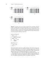
Figure 10.7 The effect of the ALLOCATE-OBJECT and FREE-OBJECT procedures. (a) The list
of Figure 10.5 (lightly shaded) and a free list (heavily shaded). Arrows show the free-list structure.
(b) The result of calling A
LLOCATE-OBJECT./ (which returns index 4), setting keyŒ4 to 25, and
calling L
IST-INSERT.L; 4/. The new free-list head is object 8, which had been nextŒ4 on the free
list. (c) After executing L
IST-DELETE.L; 5/, we call FREE-OBJECT.5/. Object 5 becomes the new
free-list head, with object 8 following it on the free list.
ALLOCATE-OBJECT./
1 if free
==
NIL
2 error “out of space”
3 else x D free
4 free D x:next
5 return x
F
REE-OBJECT.x/
1 x:next D free

2 free D x
The free list initially contains all n unallocated objects. Once the free list has been
exhausted, running the A
LLOCATE-OBJECT procedure signals an error. We can
even service several linked lists with just a single free list. Figure 10.8 shows two
linked lists and a free list intertwined through key, next,andpre arrays.
The two procedures run in O.1/ time, which makes them quite practical. We
can modify them to work for any homogeneous collection of objects by letting any
one of the attributes in the object act like a next attribute in the free list.
10.3 Implementing pointers and objects 245
12345678910
next
key
prev
free
3
62
63
715
79
9
10
48
1
L
2
L
1
k
1

k
2
k
3
k
5
k
6
k
7
k
9
Figure 10.8 Two linked lists, L
1
(lightly shaded) and L
2
(heavily shaded), and a free list (dark-
ened) intertwined.
Exercises
10.3-1
Draw a picture of the sequence h13; 4; 8; 19; 5; 11i stored as a doubly linked list
using the multiple-array representation. Do the same for the single-array represen-
tation.
10.3-2
Write the procedures A
LLOCATE-OBJECT and FREE-OBJECT for a homogeneous
collection of objects implemented by the single-array representation.
10.3-3
Why don’t we need to set or reset the pre attributes of objects in the implementa-
tion of the A

LLOCATE-OBJECT and FREE-OBJECT procedures?
10.3-4
It is often desirable to keep all elements of a doubly linked list compact in storage,
using, for example, the first m index locations in the multiple-array representation.
(This is the case in a paged, virtual-memory computing environment.) Explain
how to implement the procedures A
LLOCATE-OBJECT and FREE-OBJECT so that
the representation is compact. Assume that there are no pointers to elements of the
linked list outside the list itself. (Hint: Use the array implementation of a stack.)
10.3-5
Let L be a doubly linked list of length n stored in arrays key, pre,andnext of
length m. Suppose that these arrays are managed by A
LLOCATE-OBJECT and
FREE-OBJECT procedures that keep a doubly linked free list F . Suppose further
that of the m items, exactly n are on list L and m  n are on the free list. Write
a procedure C
OMPACTIFY-LIST.L; F / that, given the list L and the free list F ,
moves the items in L so that they occupy array positions 1;2;:::;nand adjusts the
free list F so that it remains correct, occupying array positions nC1; n C2;:::;m.
The running time of your procedure should be ‚.n/, and it should use only a
constant amount of extra space. Argue that your procedure is correct.
246 Chapter 10 Elementary Data Structures
10.4 Representing rooted trees
The methods for representing lists given in the previous section extend to any ho-
mogeneous data structure. In this section, we look specifically at the problem of
representing rooted trees by linked data structures. We first look at binary trees,
and then we present a method for rooted trees in which nodes can have an arbitrary
number of children.
We represent each node of a tree by an object. As with linked lists, we assume
that each node contains a key attribute. The remaining attributes of interest are

pointers to other nodes, and they vary according to the type of tree.
Binary trees
Figure 10.9 shows how we use the attributes p, left,andright to store pointers to
the parent, left child, and right child of each node in a binary tree T .Ifx:p D
NIL,
then x is the root. If node x has no left child, then x:left D NIL, and similarly for
the right child. The root of the entire tree T is pointed to by the attribute T:root.If
T:root D
NIL, then the tree is empty.
Rooted trees with unbounded branching
We can extend the scheme for representing a binary tree to any class of trees in
which the number of children of each node is at most some constant k: we replace
the left and right attributes by child
1
; child
2
;:::;child
k
. This scheme no longer
works when the number of children of a node is unbounded, since we do not know
how many attributes (arrays in the multiple-array representation) to allocate in ad-
vance. Moreover, even if the number of children k is bounded by a large constant
but most nodes have a small number of children, we may waste a lot of memory.
Fortunately, there is a clever scheme to represent trees with arbitrary numbers of
children. It has the advantage of using only O.n/ space for any n-node rooted tree.
The left-child, right-sibling representation appears in Figure 10.10. As before,
each node contains a parent pointer p,andT:root points to the root of tree T .
Instead of having a pointer to each of its children, however, each node x has only
two pointers:
1. x:left-child points to the leftmost child of node x,and

2. x:right-sibling points to the sibling of x immediately to its right.
If node x has no children, then x:left-child D
NIL, and if node x is the rightmost
child of its parent, then x:right-sibling D NIL.
10.4 Representing rooted trees 247
T:root
Figure 10.9 The representation of a binary tree T . Each node x has the attributes x:p (top), x:left
(lower left), and x:right (lower right). The key attributes are not shown.
T:root
Figure 10.10 The left-child, right-sibling representation of a tree T . Each node x has attributes x:p
(top), x:left-child (lower left), and x:right-sibling (lower right). The key attributes are not shown.
248 Chapter 10 Elementary Data Structures
Other tree representations
We sometimes represent rooted trees in other ways. In Chapter 6, for example,
we represented a heap, which is based on a complete binary tree, by a single array
plus the index of the last node in the heap. The trees that appear in Chapter 21 are
traversed only toward the root, and so only the parent pointers are present; there
are no pointers to children. Many other schemes are possible. Which scheme is
best depends on the application.
Exercises
10.4-1
Draw the binary tree rooted at index 6 that is represented by the following at-
tributes:
index key left right
1127 3
2158
NIL
3410NIL
4105 9
52

NIL NIL
6181 4
77
NIL NIL
8146 2
921
NIL NIL
10 5 NIL NIL
10.4-2
Write an O.n/-time recursive procedure that, given an n-node binary tree, prints
out the key of each node in the tree.
10.4-3
Write an O.n/-time nonrecursive procedure that, given an n-node binary tree,
prints out the key of each node in the tree. Use a stack as an auxiliary data structure.
10.4-4
Write an O.n/-time procedure that prints all the keys of an arbitrary rooted tree
with n nodes, where the tree is stored using the left-child, right-sibling representa-
tion.
10.4-5 ?
Write an O.n/-time nonrecursive procedure that, given an n-node binary tree,
prints out the key of each node. Use no more than constant extra space outside
Problems for Chapter 10 249
of the tree itself and do not modify the tree, even temporarily, during the proce-
dure.
10.4-6 ?
The left-child, right-sibling representation of an arbitrary rooted tree uses three
pointers in each node: left-child, right-sibling,andparent. From any node, its
parent can be reached and identified in constant time and all its children can be
reached and identified in time linear in the number of children. Show how to use
only two pointers and one boolean value in each node so that the parent of a node

or all of its children can be reached and identified in time linear in the number of
children.
Problems
10-1 Comparisons among lists
For each of the four types of lists in the following table, what is the asymptotic
worst-case running time for each dynamic-set operation listed?
unsorted, sorted, unsorted, sorted,
singly singly doubly doubly
linked linked linked linked
SEARCH.L; k/
INSERT.L; x/
DELETE.L; x/
SUCCESSOR.L; x/
PREDECESSOR.L; x/
MINIMUM.L/
MAXIMUM.L/
250 Chapter 10 Elementary Data Structures
10-2 Mergeable heaps using linked lists
A mergeable heap supports the following operations: MAKE-HEAP (which creates
an empty mergeable heap), INSERT,MINIMUM,EXTRACT-MIN,andUNION.
1
Show how to implement mergeable heaps using linked lists in each of the following
cases. Try to make each operation as efficient as possible. Analyze the running
time of each operation in terms of the size of the dynamic set(s) being operated on.
a. Lists are sorted.
b. Lists are unsorted.
c. Lists are unsorted, and dynamic sets to be merged are disjoint.
10-3 Searching a sorted compact list
Exercise 10.3-4 asked how we might maintain an n-element list compactly in the
first n positions of an array. We shall assume that all keys are distinct and that the

compact list is also sorted, that is, keyŒi < keyŒnextŒi for all i D 1;2;:::;nsuch
that nextŒi ¤
NIL. We will also assume that we have a variable L that contains
the index of the first element on the list. Under these assumptions, you will show
that we can use the following randomized algorithm to search the list in O.
p
n/
expected time.
C
OMPACT-LIST-SEARCH.L;n;k/
1 i D L
2 while i ¤
NIL and keyŒi < k
3 j D R
ANDOM.1; n/
4 if keyŒi  < keyŒj  and keyŒj  Ä k
5 i D j
6 if keyŒi
==
k
7 return i
8 i D nextŒi
9 if i
==
NIL or keyŒi > k
10 return NIL
11 else return i
If we ignore lines 3–7 of the procedure, we have an ordinary algorithm for
searching a sorted linked list, in which index i points to each position of the list in
1

Because we have defined a mergeable heap to support MINIMUM and EXTRACT-MIN, we can also
refer to it as a mergeable min-heap. Alternatively, if it supported M
AXIMUM and EXTRACT-MAX,
it would be a mergeable max-heap.
Problems for Chapter 10 251
turn. The search terminates once the index i “falls off” the end of the list or once
keyŒi  k. In the latter case, if keyŒi D k, clearly we have found a key with the
value k. If, however, keyŒi > k, then we will never find a key with the value k,
and so terminating the search was the right thing to do.
Lines 3–7 attempt to skip ahead to a randomly chosen position j .Suchaskip
benefits us if keyŒj  is larger than keyŒi andnolargerthank; in such a case, j
marks a position in the list that i would have to reach during an ordinary list search.
Because the list is compact, we know that any choice of j between 1 and n indexes
some object in the list rather than a slot on the free list.
Instead of analyzing the performance of C
OMPACT-LIST-SEARCH directly, we
shall analyze a related algorithm, COMPACT-LIST-SEARCH
0
, which executes two
separate loops. This algorithm takes an additional parameter t which determines
an upper bound on the number of iterations of the first loop.
C
OMPACT-LIST-SEARCH
0
.L;n;k;t/
1 i D L
2 for q D 1 to t
3 j D R
ANDOM.1; n/
4 if keyŒi  < keyŒj  and keyŒj  Ä k

5 i D j
6 if keyŒi
==
k
7 return i
8 while i ¤
NIL and keyŒi  < k
9 i D nextŒi
10 if i
==
NIL or keyŒi > k
11 return NIL
12 else return i
To compare the execution of the algorithms C
OMPACT-LIST-SEARCH.L;n;k/
and COMPACT-LIST-SEARCH
0
.L;n;k;t/, assume that the sequence of integers re-
turned by the calls of RANDOM.1; n/ is the same for both algorithms.
a. Suppose that C
OMPACT-LIST-SEARCH.L;n;k/takes t iterations of the while
loop of lines 2–8. Argue that COMPACT-LIST-SEARCH
0
.L;n;k;t/returns the
same answer and that the total number of iterations of both the for and while
loops within C
OMPACT-LIST-SEARCH
0
is at least t.
In the call C

OMPACT-LIST-SEARCH
0
.L;n;k;t/,letX
t
be the random variable that
describes the distance in the linked list (that is, through the chain of next pointers)
from position i to the desired key k after t iterations of the for loop of lines 2–7
have occurred.
252 Chapter 10 Elementary Data Structures
b. Argue that the expected running time of COMPACT-LIST-SEARCH
0
.L;n;k;t/
is O.t C E ŒX
t
/.
c. Show that E ŒX
t
 Ä
P
n
rD1
.1  r=n/
t
.(Hint: Use equation (C.25).)
d. Show that
P
n1
rD0
r
t

Ä n
tC1
=.t C1/.
e. Prove that E ŒX
t
 Ä n=.t C 1/.
f. Show that C
OMPACT-LIST-SEARCH
0
.L;n;k;t/ runs in O.t C n=t/ expected
time.
g. Conclude that C
OMPACT-LIST-SEARCH runs in O.
p
n/ expected time.
h. Why do we assume that all keys are distinct in C
OMPACT-LIST-SEARCH?Ar-
gue that random skips do not necessarily help asymptotically when the list con-
tains repeated key values.
Chapter notes
Aho, Hopcroft, and Ullman [6] and Knuth [209] are excellent references for ele-
mentary data structures. Many other texts cover both basic data structures and their
implementation in a particular programming language. Examples of these types of
textbooks include Goodrich and Tamassia [147], Main [241], Shaffer [311], and
Weiss [352, 353, 354]. Gonnet [145] provides experimental data on the perfor-
mance of many data-structure operations.
The origin of stacks and queues as data structures in computer science is un-
clear, since corresponding notions already existed in mathematics and paper-based
business practices before the introduction of digital computers. Knuth [209] cites
A. M. Turing for the development of stacks for subroutine linkage in 1947.

Pointer-based data structures also seem to be a folk invention. According to
Knuth, pointers were apparently used in early computers with drum memories. The
A-1 language developed by G. M. Hopper in 1951 represented algebraic formulas
as binary trees. Knuth credits the IPL-II language, developed in 1956 by A. Newell,
J. C. Shaw, and H. A. Simon, for recognizing the importance and promoting the
use of pointers. Their IPL-III language, developed in 1957, included explicit stack
operations.
11 Hash Tables
Many applications require a dynamic set that supports only the dictionary opera-
tions INSERT,SEARCH,andDELETE. For example, a compiler that translates a
programming language maintains a symbol table, in which the keys of elements
are arbitrary character strings corresponding to identifiers in the language. A hash
table is an effective data structure for implementing dictionaries. Although search-
ing for an element in a hash table can take as long as searching for an element in a
linked list—‚.n/ time in the worst case—in practice, hashing performs extremely
well. Under reasonable assumptions, the average time to search for an element in
a hash table is O.1/.
A hash table generalizes the simpler notion of an ordinary array. Directly ad-
dressing into an ordinary array makes effective use of our ability to examine an
arbitrary position in an array in O.1/ time. Section 11.1 discusses direct address-
ing in more detail. We can take advantage of direct addressing when we can afford
to allocate an array that has one position for every possible key.
When the number of keys actually stored is small relative to the total number of
possible keys, hash tables become an effective alternative to directly addressing an
array, since a hash table typically uses an array of size proportional to the number
of keys actually stored. Instead of using the key as an array index directly, the array
index is computed from the key. Section 11.2 presents the main ideas, focusing on
“chaining” as a way to handle “collisions,” in which more than one key maps to the
same array index. Section 11.3 describes how we can compute array indices from
keys using hash functions. We present and analyze several variations on the basic

theme. Section 11.4 looks at “open addressing,” which is another way to deal with
collisions. The bottom line is that hashing is an extremely effective and practical
technique: the basic dictionary operations require only O.1/ time on the average.
Section 11.5 explains how “perfect hashing” can support searches in O.1/ worst-
case time, when the set of keys being stored is static (that is, when the set of keys
never changes once stored).
254 Chapter 11 Hash Tables
11.1 Direct-address tables
Direct addressing is a simple technique that works well when the universe U of
keys is reasonably small. Suppose that an application needs a dynamic set in which
each element has a key drawn from the universe U D
f
0; 1; : : : ; m  1
g
,wherem
is not too large. We shall assume that no two elements have the same key.
To represent the dynamic set, we use an array, or direct-address table, denoted
by TŒ0::m 1, in which each position, or slot, corresponds to a key in the uni-
verse U . Figure 11.1 illustrates the approach; slot k points to an element in the set
with key k. If the set contains no element with key k,thenTŒkD
NIL.
The dictionary operations are trivial to implement:
D
IRECT-ADDRESS-SEARCH.T; k/
1 return TŒk
D
IRECT-ADDRESS-INSERT.T; x/
1 TŒx:key D x
D
IRECT-ADDRESS-DELETE.T; x/

1 TŒx:key D
NIL
Each of these operations takes only O.1/ time.
T
U
(universe of keys)
K
(actual
keys)
2
3
5
8
1
9
4
0
7
6
2
3
5
8
key satellite data
2
0
1
3
4
5

6
7
8
9
Figure 11.1 How to implement a dynamic set by a direct-address table T . Each key in the universe
U D
f
0; 1; : : : ; 9
g
corresponds to an index in the table. The set K D
f
2; 3; 5; 8
g
of actual keys
determines the slots in the table that contain pointers to elements. The other slots, heavily shaded,
contain
NIL.
11.1 Direct-address tables 255
For some applications, the direct-address table itself can hold the elements in the
dynamic set. That is, rather than storing an element’s key and satellite data in an
object external to the direct-address table, with a pointer from a slot in the table to
the object, we can store the object in the slot itself, thus saving space. We would
use a special key within an object to indicate an empty slot. Moreover, it is often
unnecessary to store the key of the object, since if we have the index of an object
in the table, we have its key. If keys are not stored, however, we must have some
way to tell whether the slot is empty.
Exercises
11.1-1
Suppose that a dynamic set S is represented by a direct-address table T of length m.
Describe a procedure that finds the maximum element of S . What is the worst-case

performance of your procedure?
11.1-2
A bit vector is simply an array of bits (0sand1s). A bit vector of length m takes
much less space than an array of m pointers. Describe how to use a bit vector
to represent a dynamic set of distinct elements with no satellite data. Dictionary
operations should run in O.1/ time.
11.1-3
Suggest how to implement a direct-address table in which the keys of stored el-
ements do not need to be distinct and the elements can have satellite data. All
three dictionary operations (I
NSERT,DELETE,andSEARCH) should run in O.1/
time. (Don’t forget that DELETE takes as an argument a pointer to an object to be
deleted, not a key.)
11.1-4 ?
We wish to implement a dictionary by using direct addressing on a huge array. At
the start, the array entries may contain garbage, and initializing the entire array
is impractical because of its size. Describe a scheme for implementing a direct-
address dictionary on a huge array. Each stored object should use O.1/ space;
the operations S
EARCH,INSERT,andDELETE should take O.1/ time each; and
initializing the data structure should take O.1/ time. (Hint: Use an additional array,
treated somewhat like a stack whose size is the number of keys actually stored in
the dictionary, to help determine whether a given entry in the huge array is valid or
not.)
256 Chapter 11 Hash Tables
11.2 Hash tables
The downside of direct addressing is obvious: if the universe U is large, storing
atableT of size
j
U

j
may be impractical, or even impossible, given the memory
available on a typical computer. Furthermore, the set K of keys actually stored
may be so small relative to U that most of the space allocated for T would be
wasted.
When the set K of keys stored in a dictionary is much smaller than the uni-
verse U of all possible keys, a hash table requires much less storage than a direct-
address table. Specifically, we can reduce the storage requirement to ‚.
j
K
j
/ while
we maintain the benefit that searching for an element in the hash table still requires
only O.1/ time. The catch is that this bound is for the average-case time, whereas
for direct addressing it holds for the worst-case time.
With direct addressing, an element with key k is stored in slot k. With hashing,
this element is stored in slot h.k/; that is, we use a hash function h to compute the
slot from the key k. Here, h maps the universe U of keys into the slots of a hash
table TŒ0::m 1:
h W U !
f
0; 1; : : : ; m  1
g
;
where the size m of the hash table is typically much less than
j
U
j
. We say that an
element with key k hashes to slot h.k/; we also say that h.k/ is the hash value of

key k. Figure 11.2 illustrates the basic idea. The hash function reduces the range
of array indices and hence the size of the array. Instead of a size of
j
U
j
, the array
can have size
m.
T
U
(universe of keys)
K
(actual
keys)
0
m–1
k
1
k
2
k
3
k
4
k
5
h(k
1
)
h(k

4
)
h(k
3
)
h(k
2
) = h(k
5
)
Figure 11.2 Using a hash function h to map keys to hash-table slots. Because keys k
2
and k
5
map
to the same slot, they collide.
11.2 Hash tables 257
T
U
(universe of keys)
K
(actual
keys)
k
1
k
2
k
3
k

4
k
5
k
6
k
7
k
8
k
1
k
2
k
3
k
4
k
5
k
6
k
7
k
8
Figure 11.3 Collision resolution by chaining. Each hash-table slot TŒjcontains a linked list of
all the keys whose hash value is j . For example, h.k
1
/ D h.k
4

/ and h.k
5
/ D h.k
7
/ D h.k
2
/.
The linked list can be either singly or doubly linked; we show it as doubly linked because deletion is
faster that way.
There is one hitch: two keys may hash to the same slot. We call this situation
a collision. Fortunately, we have effective techniques for resolving the conflict
created by collisions.
Of course, the ideal solution would be to avoid collisions altogether. We might
try to achieve this goal by choosing a suitable hash function h. One idea is to
make h appear to be “random,” thus avoiding collisions or at least minimizing
their number. The very term “to hash,” evoking images of random mixing and
chopping, captures the spirit of this approach. (Of course, a hash function h must be
deterministic in that a given input k should always produce the same output h.k/.)
Because
j
U
j
>m, however, there must be at least two keys that have the same hash
value; avoiding collisions altogether is therefore impossible. Thus, while a well-
designed, “random”-looking hash function can minimize the number of collisions,
we still need a method for resolving the collisions that do occur.
The remainder of this section presents the simplest collision resolution tech-
nique, called chaining. Section 11.4 introduces an alternative method for resolving
collisions, called open addressing.
Collision resolution by chaining

In chaining, we place all the elements that hash to the same slot into the same
linked list, as Figure 11.3 shows. Slot j contains a pointer to the head of the list of
all stored elements that hash to j ; if there are no such elements, slot j contains
NIL.
258 Chapter 11 Hash Tables
The dictionary operations on a hash table T are easy to implement when colli-
sions are resolved by chaining:
C
HAINED-HASH-INSERT.T; x/
1 insert x at the head of list TŒh.x:key/
C
HAINED-HASH-SEARCH.T; k/
1 search for an element with key k in list TŒh.k/
C
HAINED-HASH-DELETE.T; x/
1 delete x from the list TŒh.x:key/
The worst-case running time for insertion is O.1/. The insertion procedure is fast
in part because it assumes that the element x being inserted is not already present in
the table; if necessary, we can check this assumption (at additional cost) by search-
ing for an element whose key is x:key before we insert. For searching, the worst-
case running time is proportional to the length of the list; we shall analyze this
operation more closely below. We can delete an element in O.1/ time if the lists
are doubly linked, as Figure 11.3 depicts. (Note that C
HAINED-HASH-DELETE
takes as input an element x and not its key k, so that we don’t have to search for x
first. If the hash table supports deletion, then its linked lists should be doubly linked
so that we can delete an item quickly. If the lists were only singly linked, then to
delete element x, we would first have to find x in the list TŒh.x:key/ so that we
could update the next attribute of x’s predecessor. With singly linked lists, both
deletion and searching would have the same asymptotic running times.)

Analysis of hashing with chaining
How well does hashing with chaining perform? In particular, how long does it take
to search for an element with a given key?
Given a hash table T with m slots that stores n elements, we define the load
factor ˛ for T as n=m, that is, the average number of elements stored in a chain.
Our analysis will be in terms of ˛, which can be less than, equal to, or greater
than 1.
The worst-case behavior of hashing with chaining is terrible: all n keys hash
to the same slot, creating a list of length n. The worst-case time for searching is
thus ‚.n/ plus the time to compute the hash function—no better than if we used
one linked list for all the elements. Clearly, we do not use hash tables for their
worst-case performance. (Perfect hashing, described in Section 11.5, does provide
good worst-case performance when the set of keys is static, however.)
The average-case performance of hashing depends on how well the hash func-
tion h distributes the set of keys to be stored among the m slots, on the average.
11.2 Hash tables 259
Section 11.3 discusses these issues, but for now we shall assume that any given
element is equally likely to hash into any of the m slots, independently of where
any other element has hashed to. We call this the assumption of simple uniform
hashing.
For j D 0; 1; : : : ; m  1, let us denote the length of the list TŒjby n
j
,sothat
n D n
0
C n
1
CCn
m1
; (11.1)

and the expected value of n
j
is E Œn
j
 D ˛ D n=m.
We assume that O.1/ time suffices to compute the hash value h.k/,sothat
the time required to search for an element with key k depends linearly on the
length n
h.k/
of the list TŒh.k/. Setting aside the O.1/ time required to compute
the hash function and to access slot h.k/, let us consider the expected number of
elements examined by the search algorithm, that is, the number of elements in the
list TŒh.k/that the algorithm checks to see whether any have a key equal to k.We
shall consider two cases. In the first, the search is unsuccessful: no element in the
table has key k. In the second, the search successfully finds an element with key k.
Theorem 11.1
In a hash table in which collisions are resolved by chaining, an unsuccessful search
takes average-case time ‚.1C˛/, under the assumption of simple uniform hashing.
Proof Under the assumption of simple uniform hashing, any key k not already
stored in the table is equally likely to hash to any of the m slots. The expected time
to search unsuccessfully for a key k is the expected time to search to the end of
list TŒh.k/, which has expected length E Œn
h.k/
 D ˛. Thus, the expected number
of elements examined in an unsuccessful search is ˛, and the total time required
(including the time for computing h.k/)is‚.1 C ˛/.
The situation for a successful search is slightly different, since each list is not
equally likely to be searched. Instead, the probability that a list is searched is pro-
portional to the number of elements it contains. Nonetheless, the expected search
time still turns out to be ‚.1 C ˛/.

Theorem 11.2
In a hash table in which collisions are resolved by chaining, a successful search
takes average-case time ‚.1C˛/, under the assumption of simple uniform hashing.
Proof We assume that the element being searched for is equally likely to be any
of the n elements stored in the table. The number of elements examined during a
successful search for an element x is one more than the number of elements that
260 Chapter 11 Hash Tables
appear before x in x’s list. Because new elements are placed at the front of the
list, elements before x in the list were all inserted after x was inserted. To find
the expected number of elements examined, we take the average, over the n ele-
ments x in the table, of 1 plus the expected number of elements added to x’s list
after x was added to the list. Let x
i
denote the ith element inserted into the ta-
ble, for i D 1;2;:::;n,andletk
i
D x
i
:key. For keys k
i
and k
j
,wedefinethe
indicator random variable X
ij
D I
f
h.k
i
/ D h.k

j
/
g
. Under the assumption of sim-
ple uniform hashing, we have Pr
f
h.k
i
/ D h.k
j
/
g
D 1=m, and so by Lemma 5.1,
E ŒX
ij
 D 1=m. Thus, the expected number of elements examined in a successful
search is
E
"
1
n
n
X
iD1

1 C
n
X
j DiC1
X

ij
!#
D
1
n
n
X
iD1

1 C
n
X
j DiC1
E ŒX
ij

!
(by linearity of expectation)
D
1
n
n
X
iD1

1 C
n
X
j DiC1
1

m
!
D 1 C
1
nm
n
X
iD1
.n i/
D 1 C
1
nm

n
X
iD1
n 
n
X
iD1
i
!
D 1 C
1
nm
Â
n
2

n.n C1/

2
Ã
(by equation (A.1))
D 1 C
n 1
2m
D 1 C
˛
2

˛
2n
:
Thus, the total time required for a successful search (including the time for com-
puting the hash function) is ‚.2 C ˛=2  ˛=2n/ D ‚.1 C˛/.
What does this analysis mean? If the number of hash-table slots is at least pro-
portional to the number of elements in the table, we have n D O.m/ and, con-
sequently, ˛ D n=m D O.m/=m D O.1/. Thus, searching takes constant time
on average. Since insertion takes O.1/ worst-case time and deletion takes O.1/
worst-case time when the lists are doubly linked, we can support all dictionary
operations in O.1/ time on average.
11.2 Hash tables 261
Exercises
11.2-1
Suppose we use a hash function h to hash n distinct keys into an array T of
length m. Assuming simple uniform hashing, what is the expected number of
collisions? More precisely, what is the expected cardinality of
ff
k; l
g

W k ¤ l and
h.k/ D h.l/
g
?
11.2-2
Demonstrate what happens when we insert the keys 5; 28; 19; 15; 20; 33; 12; 17; 10
into a hash table with collisions resolved by chaining. Let the table have 9 slots,
and let the hash function be h.k/ D k mod 9.
11.2-3
Professor Marley hypothesizes that he can obtain substantial performance gains by
modifying the chaining scheme to keep each list in sorted order. How does the pro-
fessor’s modification affect the running time for successful searches, unsuccessful
searches, insertions, and deletions?
11.2-4
Suggest how to allocate and deallocate storage for elements within the hash table
itself by linking all unused slots into a free list. Assume that one slot can store
a flag and either one element plus a pointer or two pointers. All dictionary and
free-list operations should run in O.1/ expected time. Does the free list need to be
doubly linked, or does a singly linked free list suffice?
11.2-5
Suppose that we are storing a set of n keys into a hash table of size m. Show that if
the keys are drawn from a universe U with
j
U
j
>nm,thenU has a subset of size n
consisting of keys that all hash to the same slot, so that the worst-case searching
time for hashing with chaining is ‚.n/.
11.2-6
Suppose we have stored n keys in a hash table of size m, with collisions resolved by

chaining, and that we know the length of each chain, including the length L of the
longest chain. Describe a procedure that selects a key uniformly at random from
among the keys in the hash table and returns it in expected time O.L  .1 C 1=˛//.
262 Chapter 11 Hash Tables
11.3 Hash functions
In this section, we discuss some issues regarding the design of good hash functions
and then present three schemes for their creation. Two of the schemes, hashing by
division and hashing by multiplication, are heuristic in nature, whereas the third
scheme, universal hashing, uses randomization to provide provably good perfor-
mance.
What makes a good hash function?
A good hash function satisfies (approximately) the assumption of simple uniform
hashing: each key is equally likely to hash to any of the m slots, independently of
where any other key has hashed to. Unfortunately, we typically have no way to
check this condition, since we rarely know the probability distribution from which
the keys are drawn. Moreover, the keys might not be drawn independently.
Occasionally we do know the distribution. For example, if we know that the
keys are random real numbers k independently and uniformly distributed in the
range 0 Ä k<1, then the hash function
h.k/ D
b
km
c
satisfies the condition of simple uniform hashing.
In practice, we can often employ heuristic techniques to create a hash function
that performs well. Qualitative information about the distribution of keys may be
useful in this design process. For example, consider a compiler’s symbol table, in
which the keys are character strings representing identifiers in a program. Closely
related symbols, such as pt and pts, often occur in the same program. A good
hash function would minimize the chance that such variants hash to the same slot.

A good approach derives the hash value in a way that we expect to be indepen-
dent of any patterns that might exist in the data. For example, the “division method”
(discussed in Section 11.3.1) computes the hash value as the remainder when the
key is divided by a specified prime number. This method frequently gives good
results, assuming that we choose a prime number that is unrelated to any patterns
in the distribution of keys.
Finally, we note that some applications of hash functions might require stronger
properties than are provided by simple uniform hashing. For example, we might
want keys that are “close” in some sense to yield hash values that are far apart.
(This property is especially desirable when we are using linear probing, defined in
Section 11.4.) Universal hashing, described in Section 11.3.3, often provides the
desired properties.
11.3 Hash functions 263
Interpreting keys as natural numbers
Most hash functions assume that the universe of keys is the set N D
f
0; 1; 2; : : :
g
of natural numbers. Thus, if the keys are not natural numbers, we find a way to
interpret them as natural numbers. For example, we can interpret a character string
as an integer expressed in suitable radix notation. Thus, we might interpret the
identifier pt as the pair of decimal integers .112; 116/,sincep D 112 and t D 116
in the ASCII character set; then, expressed as a radix-128 integer, pt becomes
.112  128/ C 116 D 14452. In the context of a given application, we can usually
devise some such method for interpreting each key as a (possibly large) natural
number. In what follows, we assume that the keys are natural numbers.
11.3.1 The division method
In the division method for creating hash functions, we map a key k into one of m
slots by taking the remainder of k divided by m. That is, the hash function is
h.k/ D k mod m:

For example, if the hash table has size m D 12 and the key is k D 100,then
h.k/ D 4. Since it requires only a single division operation, hashing by division is
quite fast.
When using the division method, we usually avoid certain values of m.For
example, m should not be a power of 2, since if m D 2
p
,thenh.k/ is just the p
lowest-order bits of k. Unless we know that all low-order p-bit patterns are equally
likely, we are better off designing the hash function to depend on all the bits of the
key. As Exercise 11.3-3 asks you to show, choosing m D 2
p
 1 when k is a
character string interpreted in radix 2
p
may be a poor choice, because permuting
the characters of k does not change its hash value.
A prime not too close to an exact power of 2 is often a good choice for m.For
example, suppose we wish to allocate a hash table, with collisions resolved by
chaining, to hold roughly n D 2000 character strings, where a character has 8 bits.
We don’t mind examining an average of 3 elements in an unsuccessful search, and
so we allocate a hash table of size m D 701. We could choose m D 701 because
it is a prime near 2000=3 but not near any power of 2. Treating each key k as an
integer, our hash function would be
h.k/ D k mod 701 :
11.3.2 The multiplication method
The multiplication method for creating hash functions operates in two steps. First,
we multiply the key k by a constant A in the range 0<A<1and extract the
264 Chapter 11 Hash Tables
×
s D A 2

w
w bits
k
r
0
r
1
h.k/
extract p bits
Figure 11.4 The multiplication method of hashing. The w-bit representation of the key k is multi-
plied by the w-bit value s D A  2
w
.Thep highest-order bits of the lower w-bit half of the product
form the desired hash value h.k/.
fractional part of kA. Then, we multiply this value by m and take the floor of the
result. In short, the hash function is
h.k/ D
b
m.kAmod 1/
c
;
where “kA mod 1” means the fractional part of kA,thatis,kA 
b
kA
c
.
An advantage of the multiplication method is that the value of m is not critical.
We typically choose it to be a power of 2 (m D 2
p
for some integer p), since we

can then easily implement the function on most computers as follows. Suppose
that the word size of the machine is w bits and that k fits into a single word. We
restrict A to be a fraction of the form s=2
w
,wheres is an integer in the range
0<s<2
w
. Referring to Figure 11.4, we first multiply k by the w-bit integer
s D A 2
w
. The result is a 2w-bit value r
1
2
w
Cr
0
,wherer
1
is the high-order word
of the product and r
0
is the low-order word of the product. The desired p-bit hash
value consists of the p most significant bits of r
0
.
Although this method works with any value of the constant A, it works better
with some values than with others. The optimal choice depends on the character-
istics of the data being hashed. Knuth [211] suggests that
A  .
p

5 1/=2 D 0:6180339887 : : : (11.2)
is likely to work reasonably well.
As an example, suppose we have k D 123456, p D 14, m D 2
14
D 16384,
and w D 32. Adapting Knuth’s suggestion, we choose A to be the fraction of the
form s=2
32
that is closest to .
p
5  1/=2,sothatA D 2654435769=2
32
.Then
k  s D 327706022297664 D .76300  2
32
/ C 17612864,andsor
1
D 76300
and r
0
D 17612864.The14 most significant bits of r
0
yield the value h.k/ D 67.
11.3 Hash functions 265
? 11.3.3 Universal hashing
If a malicious adversary chooses the keys to be hashed by some fixed hash function,
then the adversary can choose n keys that all hash to the same slot, yielding an av-
erage retrieval time of ‚.n/. Any fixed hash function is vulnerable to such terrible
worst-case behavior; the only effective way to improve the situation is to choose
the hash function randomly in a way that is independent of the keys that are actually

going to be stored. This approach, called universal hashing, can yield provably
good performance on average, no matter which keys the adversary chooses.
In universal hashing, at the beginning of execution we select the hash function
at random from a carefully designed class of functions. As in the case of quick-
sort, randomization guarantees that no single input will always evoke worst-case
behavior. Because we randomly select the hash function, the algorithm can be-
have differently on each execution, even for the same input, guaranteeing good
average-case performance for any input. Returning to the example of a compiler’s
symbol table, we find that the programmer’s choice of identifiers cannot now cause
consistently poor hashing performance. Poor performance occurs only when the
compiler chooses a random hash function that causes the set of identifiers to hash
poorly, but the probability of this situation occurring is small and is the same for
any set of identifiers of the same size.
Let H be a finite collection of hash functions that map a given universe U of
keys into the range
f
0; 1; : : : ; m  1
g
. Such a collection is said to be universal
if for each pair of distinct keys k;l 2 U , the number of hash functions h 2 H
for which h.k/ D h.l/ is at most
j
H
j
=m. In other words, with a hash function
randomly chosen from H , the chance of a collision between distinct keys k and l
is no more than the chance 1=m of a collision if h.k/ and h.l/ were randomly and
independently chosen from the set
f
0; 1; : : : ; m  1

g
.
The following theorem shows that a universal class of hash functions gives good
average-case behavior. Recall that n
i
denotes the length of list TŒi.
Theorem 11.3
Suppose that a hash function h is chosen randomly from a universal collection of
hash functions and has been used to hash n keys into a table T of size m,us-
ing chaining to resolve collisions. If key k is not in the table, then the expected
length E Œn
h.k/
 of the list that key k hashes to is at most the load factor ˛ D n=m.
If key k is in the table, then the expected length E Œn
h.k/
 of the list containing key k
is at most 1 C ˛.
Proof We note that the expectations here are over the choice of the hash func-
tion and do not depend on any assumptions about the distribution of the keys.
For each pair k and l of distinct keys, define the indicator random variable
266 Chapter 11 Hash Tables
X
kl
D I
f
h.k/ D h.l/
g
. Since by the definition of a universal collection of hash
functions, a single pair of keys collides with probability at most 1=m,wehave
Pr

f
h.k/ D h.l/
g
Ä 1=m. By Lemma 5.1, therefore, we have E ŒX
kl
 Ä 1=m.
Next we define, for each key k, the random variable Y
k
that equals the number
of keys other than k that hash to the same slot as k,sothat
Y
k
D
X
l2T
l¤k
X
kl
:
Thus we have
E ŒY
k
 D E
2
4
X
l2T
l¤k
X
kl

3
5
D
X
l2T
l¤k
E ŒX
kl
 (by linearity of expectation)
Ä
X
l2T
l¤k
1
m
:
The remainder of the proof depends on whether key k is in table T .

If k 62 T ,thenn
h.k/
D Y
k
and
jf
l W l 2 T and l ¤ k
gj
D n. Thus E Œn
h.k/
 D
E ŒY

k
 Ä n=m D ˛.

If k 2 T , then because key k appears in list TŒh.k/and the count Y
k
does not
include key k,wehaven
h.k/
D Y
k
C 1 and
jf
l W l 2 T and l ¤ k
gj
D n  1.
Thus E Œn
h.k/
 D E ŒY
k
 C1 Ä .n  1/=m C 1 D 1 C˛  1=m < 1 C ˛.
The following corollary says universal hashing provides the desired payoff: it
has now become impossible for an adversary to pick a sequence of operations that
forces the worst-case running time. By cleverly randomizing the choice of hash
function at run time, we guarantee that we can process every sequence of operations
with a good average-case running time.
Corollary 11.4
Using universal hashing and collision resolution by chaining in an initially empty
table with m slots, it takes expected time ‚.n/ to handle any sequence of n I
NSERT,
SEARCH,andDELETE operations containing O.m/ INSERT operations.

Proof Since the number of insertions is O.m/,wehaven D O.m/ and so
˛ D O.1/.TheI
NSERT and DELETE operations take constant time and, by The-
orem 11.3, the expected time for each SEARCH operation is O.1/. By linearity of
11.3 Hash functions 267
expectation, therefore, the expected time for the entire sequence of n operations
is O.n/. Since each operation takes .1/ time, the ‚.n/ bound follows.
Designing a univ ersal class of hash functions
It is quite easy to design a universal class of hash functions, as a little number
theory will help us prove. You may wish to consult Chapter 31 first if you are
unfamiliar with number theory.
We begin by choosing a prime number p large enough so that every possible
key k is in the range 0 to p 1, inclusive. Let Z
p
denote the set
f
0; 1; : : : ; p  1
g
,
and let Z

p
denote the set
f
1;2;:::;p 1
g
.Sincep is prime, we can solve equa-
tions modulo p with the methods given in Chapter 31. Because we assume that the
size of the universe of keys is greater than the number of slots in the hash table, we
have p>m.

We now define the hash function h
ab
for any a 2 Z

p
and any b 2 Z
p
using a
linear transformation followed by reductions modulo p and then modulo m:
h
ab
.k/ D ak C b/ mod p/ mod m: (11.3)
For example, with p D 17 and m D 6,wehaveh
3;4
.8/ D 5. The family of all
such hash functions is
H
pm
D
˚
h
ab
W a 2 Z

p
and b 2 Z
p
«
: (11.4)
Each hash function h

ab
maps Z
p
to Z
m
. This class of hash functions has the nice
property that the size m of the output range is arbitrary—not necessarily prime—a
feature which we shall use in Section 11.5. Since we have p  1 choices for a
and p choices for b, the collection H
pm
contains p.p  1/ hash functions.
Theorem 11.5
The class H
pm
of hash functions defined by equations (11.3) and (11.4) is universal.
Proof Consider two distinct keys k and l from Z
p
,sothatk ¤ l.Foragiven
hash function h
ab
we let
r D .ak C b/ mod p;
s D .al C b/ mod p:
We first note that r ¤ s. Why? Observe that
r  s Á a.k  l/ .mod p/ :
It follows that r ¤ s because p is prime and both a and .k  l/ are nonzero
modulo p, and so their product must also be nonzero modulo p by Theorem 31.6.
Therefore, when computing any h
ab
2 H

pm
, distinct inputs k and l map to distinct
268 Chapter 11 Hash Tables
values r and s modulo p; there are no collisions yet at the “mod p level.” Moreover,
each of the possible p.p1/ choices for the pair .a; b/ with a ¤ 0 yields a different
resulting pair .r; s/ with r ¤ s, since we can solve for a and b given r and s:
a D

.r  s/ k  l/
1
mod p/

mod p;
b D .r ak/ mod p;
where k  l/
1
mod p/ denotes the unique multiplicative inverse, modulo p,
of k  l. Since there are only p.p  1/ possible pairs .r; s/ with r ¤ s,there
is a one-to-one correspondence between pairs .a; b/ with a ¤ 0 and pairs .r; s/
with r ¤ s. Thus, for any given pair of inputs k and l,ifwepick.a; b/ uniformly
at random from Z

p
Z
p
, the resulting pair .r; s/ is equally likely to be any pair of
distinct values modulo p.
Therefore, the probability that distinct keys k and l collide is equal to the prob-
ability that r Á s.mod m/ when r and s are randomly chosen as distinct values
modulo p.Foragivenvalueofr,ofthep 1 possible remaining values for s,the

number of values s such that s ¤ r and s Á r.mod m/ is at most
d
p=m
e
 1 Ä p C m 1/=m/ 1 (by inequality (3.6))
D .p 1/=m :
The probability that s collides with r when reduced modulo m is at most
p 1/=m/=.p  1/ D 1=m.
Therefore, for any pair of distinct values k; l 2 Z
p
,
Pr
f
h
ab
.k/ D h
ab
.l/
g
Ä 1=m ;
so that H
pm
is indeed universal.
Exercises
11.3-1
Suppose we wish to search a linked list of length n, where each element contains
akeyk along with a hash value h.k/. Each key is a long character string. How
might we take advantage of the hash values when searching the list for an element
with a given key?
11.3-2

Suppose that we hash a string of r characters into m slots by treating it as a
radix-128 number and then using the division method. We can easily represent
the number m as a 32-bit computer word, but the string of r characters, treated as
a radix-128 number, takes many words. How can we apply the division method to
compute the hash value of the character string without using more than a constant
number of words of storag
e
outside the string itself?