Mastering Excel 2003 Programming with VBA phần 4 ppt
Bạn đang xem bản rút gọn của tài liệu. Xem và tải ngay bản đầy đủ của tài liệu tại đây (2.72 MB, 61 trang )
4281book.fm Page 164 Sunday, February 29, 2004 5:12 PM
164
CHAPTER 8 THE MOST IMPORTANT OBJECT
You can apply many different techniques for moving around a worksheet. I’ll present a few here
that I’ve used successfully for many different purposes. The two primary ways to move about a work-
sheet are using the Cells property of the Worksheet object and the Offset property of the Range
object. I’ve already talked about the Cells property earlier in the chapter (see Listing 8.2), so let’s take
a look at the Offset property.
Offset Is for Relative Navigation
You can use the Offset property of the Range object to refer to ranges on a worksheet based on, or
relative to, another range. This property provides you with a great deal of flexibility for moving
around a worksheet.
One thing that you can do with Offset is process a structured list. By structured list, I mean a list
of items on a worksheet in which you know the order or structure of the columns ahead of time.
Consider the list of items shown in Figure 8.8.
One way you could process this list is by setting a reference to the first column of the first row in
the list. Then you could loop through the list, advancing your reference down a row, and terminating the
loop when you reach an empty row (assuming you know that there won’t be any empty rows within
the boundaries of your list). As you loop through the list, you could investigate columns of interest
by using the Offset property.
Listing 8.6 demonstrates how you could filter this list. You’ll have to bear with me and pretend
that Excel doesn’t have any native filtering functionality (which we’ll examine in the next chapter).
Anyway, Listing 8.6 uses the Offset property to process the list shown in Figure 8.8 so that it hides
any rows that contain cars from the 20th century. Further, this process highlights the mileage column
if the car has less than 40,000 miles.
Figure 8.8
A simple
worksheet list
4281book.fm Page 165 Sunday, February 29, 2004 5:12 PM
165
FINDING MY WAY
Listing 8.6: List Processing with the Offset Property
Sub ListExample()
FilterYear 2000
End Sub
Sub Reset()
With ThisWorkbook.Worksheets("List Example")
.Rows.Hidden = False
.Rows.Font.Bold = False
.Rows(1).Font.Bold = True
End With
End Sub
Sub FilterYear(nYear As Integer)
Dim rg As Range
Dim nMileageOffset As Integer
' 1st row is column header so start
' with 2nd row
Set rg = ThisWorkbook.Worksheets("List Example").Range("A2")
nMileageOffset = 6
' go until we bump into first
' empty cell
Do Until IsEmpty(rg)
If rg.Value < nYear Then
rg.EntireRow.Hidden = True
Else
' check milage
If rg.Offset(0, nMileageOffset).Value < 40000 Then
rg.Offset(0, nMileageOffset).Font.Bold = True
Else
rg.Offset(0, nMileageOffset).Font.Bold = False
End If
rg.EntireRow.Hidden = False
End If
' move down to the next row
Set rg = rg.Offset(1, 0)
Loop
Set rg = Nothing
End Sub
4281book.fm Page 166 Sunday, February 29, 2004 5:12 PM
166
CHAPTER 8 THE MOST IMPORTANT OBJECT
Let me make a few comments before I analyze this listing. First, this listing uses a worksheet named
“List Example” and doesn’t validate this assumption, so be sure you have either changed the worksheet
name in the code or named one of your worksheets “List Example”. Then run the ListExample proce-
dure to hide selected rows and the Reset procedure to display the worksheet as it originally appeared.
The heart of this example is the poorly named FilterYear procedure. Notice one of the variables
is named nMileageOffset. The procedure uses the Offset property to observe the value in the Mileage
column. Your Range object variable, rg, is located in column 1, so to use Offset to view the Mileage
column, you need to look in the cell six columns to the right. It’s a good idea, at a minimum, to store
a value like this in a variable or a constant. That way if you need to change the value (perhaps you need
to insert a column, for example), you only have to change it in one location. The FilterYear stores this
mileage column offset in a variable named nMileageOffset.
The processing loop is a Do…Loop that terminates when it finds an empty cell. Each time through the
loop, you set the rg variable to refer to the next cell down. The primary assumption that is made here is that
you don’t have any empty cells between the first and last row. If there is a chance that you may have empty
cells, you need to use another method to process the list or put some appropriate checks in place.
The first piece of business inside the loop is to see if the value in the year column (the value in the
range to which the rg variable refers) is less than the value passed in the nYear parameter. If it is, you
can use the EntireRow property of your Range object to refer to a range that represents all of the cells
in the row occupied by the rg variable. In the same statement, set the Hidden property to true to hide
the row. If the value in the Year column is equal to or greater than nYear, check the value in the Mile-
age column and ensure that the row isn’t hidden. The last thing to do inside the loop is advance the
rg variable so that it refers to the next cell down the worksheet.
Notice in the Reset procedure that you can return a range that represents all of the rows in a work-
sheet or a selected row in the worksheet. This makes it very easy to unhide all of the rows at once. In
order to remove any bold formatting that the FilterYear procedure applied, remove any bold format-
ting from any cell on the worksheet and then go back and apply it to the first row (the column head-
ings). This is much easier and faster than looping through each cell individually and turning bold off
if it is on. The output of Listing 8.6 is shown in Figure 8.9.
Figure 8.9
List processing can
be performed very
easily with just a lit-
tle bit of code.
4281book.fm Page 167 Sunday, February 29, 2004 5:12 PM
167
FINDING MY WAY
Last but Not Least—Finding the End
One property of the Range object that is extremely useful for navigational activities is the End prop-
erty. If you are used to navigating around Excel using the Control key in conjunction with the arrow
keys, you already know how End behaves—End is the programmatic equivalent of navigating using
Control in conjunction with the arrow keys. If you don’t know what I’m talking about, it’ll be helpful
to perform the following exercise to see for yourself.
1.
On a blank worksheet in Excel, select the range A1:C10.
2.
Press the numeral 1 key and then press Ctrl+Shift+Enter to populate every cell in the range
with the value 1.
3.
Also, place the value 1 in the cells A12:A15, B14, C12, and D13:D14, as shown in Figure 8.10.
4.
Select cell A1.
5.
Press Ctrl+Down Arrow to select cell A10.
6.
Press Ctrl+Right Arrow to select cell C10.
7.
Continue experimenting with Ctrl+(Up/Down/Right/Left) Arrow until you have a good
feel for how this behaves.
The general algorithm of this functionality is as follows. If the current cell is empty, then select the
first nonempty cell in the direction specified by the arrow key. If a nonempty cell can’t be found, select
the cell next to the boundary of the worksheet.
Figure 8.10
A simple list for test-
ing the End property
4281book.fm Page 168 Sunday, February 29, 2004 5:12 PM
168
CHAPTER 8 THE MOST IMPORTANT OBJECT
If the current cell is not empty, then see if the cell next to the current cell (in the direction specified
by the arrow key) is empty. If the next cell is empty, then select the first nonempty cell. If a nonempty
cell isn’t found, select the cell next to the boundary of the worksheet. If the next cell is not empty, then
select the last cell in the range of contiguous nonempty cells.
Listing 8.7 presents an example that uses the End property. I set this procedure up using the worksheet
from the preceding exercise. You may need to update the procedure to refer to a different worksheet if you
didn’t use the first worksheet in the workbook.
Listing 8.7: Using the End Property to Navigate within a Worksheet
Sub ExperimentWithEnd()
Dim ws As Worksheet
Dim rg As Range
Set ws = ThisWorkbook.Worksheets(1)
Set rg = ws.Cells(1, 1)
ws.Cells(1, 8).Value = _
"rg.address = " & rg.Address
ws.Cells(2, 8).Value = _
"rg.End(xlDown).Address = " & rg.End(xlDown).Address
ws.Cells(3, 8).Value = _
"rg.End(xlDown).End(xlDown).Address = " & _
rg.End(xlDown).End(xlDown).Address
ws.Cells(4, 8).Value = _
"rg.End(xlToRight).Address = " & rg.End(xlToRight).Address
Set rg = Nothing
Set ws = Nothing
End Sub
Listing 8.7 simply uses the End property to navigate to a few locations. It outputs the address of
the range it navigates to as it goes. Notice that because the End property returns a Range object, you
can use it multiple times in the same statement.
As you can see, using End is an efficient technique for finding the boundaries of a contiguous series
of cells that contain values. It’s also useful for finding the last row in a given column or the last column
in a given row. When you use End to find the last used cell in a column or row, however, you need
to be wary of empty cells.
In order to account for the possibility of empty cells, all you need to do to find the last cell is start
at the boundary of the worksheet. So if you need to find the last row in a given column, use End,
except start at the bottom of the worksheet. Similarly, to find the last column in a given row, start at
the far right column of the worksheet.
4281book.fm Page 169 Sunday, February 29, 2004 5:12 PM
169
FINDING MY WAY
Listing 8.8 presents two functions that return either a range that represents the last used cell in a
column or the last used cell in a row, depending on which function you call.
Listing 8.8: Finding the Last Used Cell in a Column or Row
' returns a range object that represents the last
' non-empty cell in the same column
Function GetLastCellInColumn(rg As Range) As Range
Dim lMaxRows As Long
lMaxRows = ThisWorkbook.Worksheets(1).Rows.Count
' make sure the last cell in the column is empty
If IsEmpty(rg.Parent.Cells(lMaxRows, rg.Column)) Then
Set GetLastCellInColumn = _
rg.Parent.Cells(lMaxRows, rg.Column).End(xlUp)
Else
Set GetLastCellInColumn = rg.Parent.Cells(lMaxRows, rg.Column)
End If
End Function
' returns a range object that represents the last
' non-empty cell in the same row
Function GetLastCellInRow(rg As Range) As Range
Dim lMaxColumns As Long
lMaxColumns = ThisWorkbook.Worksheets(1).Columns.Count
' make sure the last cell in the row is empty
If IsEmpty(rg.Parent.Cells(rg.Row, lMaxColumns)) Then
Set GetLastCellInRow = _
rg.Parent.Cells(rg.Row, lMaxColumns).End(xlToLeft)
Else
Set GetLastCellInRow = rg.Parent.Cells(rg.Row, lMaxColumns)
End If
End Function
GetLastCellInColumn and GetLastCellInRow work almost identically, but are different in two ways.
First, when you’re looking for the last used cell in a column, you need to start at the bottom of the work-
sheet. For rows, you start at the far right edge of the worksheet instead. The second difference is the
parameter you supply to the End property. For the last used cell in a column, you use xlUp; for the last
used cell in a row you use xlToLeft. The most important statement in each of these functions is the one
that uses the End property. I took the example shown here from the GetLastCellInRow function.
rg.Parent.Cells(rg.Row, lMaxColumns).End(xlToLeft)
4281book.fm Page 170 Sunday, February 29, 2004 5:12 PM
170
CHAPTER 8 THE MOST IMPORTANT OBJECT
The rg variable is a Range object supplied to the function as a parameter. Your objective with this
statement is to move to the last possible cell in the row to which rg belongs and then use End to move
to the first nonempty cell in the same row. You can see exactly how this objective is achieved by breaking
the statement down from left to right:
1.
First you receive a reference from rg.Parent to the worksheet that contains the range.
2.
Next you use the Cells property of the worksheet object to specify the last possible cell in the
row. Specify the specific cell by supplying a row number and a column number.
1.
You can determine the specific row number by using the Row property of the Range
object.
2.
You can determine the last possible column by counting the number of columns on a
worksheet. This is performed a few statements earlier and the result is assigned to the
lMaxColumns variable.
3.
Finally, use the End property to find the last nonempty cell in the row.
This is a good example of how you can get a lot done with one statement. As you progress and get
more familiar with the Excel object model, putting these statements together will become second
nature for you. 99 percent of the time, this statement alone would suffice. In order to account for the
possibility that the last possible cell in the row or column isn’t empty, you need to add an If…Then
statement to check for this condition. If the last possible cell is nonempty and you use the End prop-
erty on that cell, the function returns an incorrect result because it moves off of the cell to find the
next nonempty cell.
Listing 8.9 adopts these functions so that they can be called from a worksheet. The main change
you need to make is to return a numeric value that can be displayed on a worksheet rather than on a
Range object.
Listing 8.9: Returning the Last Used Cell in a Column or Row with Worksheet
Callable Functions
' returns a number that represents the last
' nonempty cell in the same column
' callable from a worksheet
Function GetLastUsedRow(rg As Range) As Long
Dim lMaxRows As Long
lMaxRows = ThisWorkbook.Worksheets(1).Rows.Count
If IsEmpty(rg.Parent.Cells(lMaxRows, rg.Column)) Then
GetLastUsedRow = _
rg.Parent.Cells(lMaxRows, rg.Column).End(xlUp).Row
Else
GetLastUsedRow = rg.Parent.Cells(lMaxRows, rg.Column).Row
End If
End Function
4281book.fm Page 171 Sunday, February 29, 2004 5:12 PM
171
INPUT EASY; OUTPUT EASIER
' returns a number that represents the last
' nonempty cell in the same row
' callable from a worksheet
Function GetLastUsedColumn(rg As Range) As Long
Dim lMaxColumns As Long
lMaxColumns = ThisWorkbook.Worksheets(1).Columns.Count
If IsEmpty(rg.Parent.Cells(rg.Row, lMaxColumns)) Then
GetLastUsedColumn = _
rg.Parent.Cells(rg.Row, lMaxColumns).End(xlToLeft).Column
Else
GetLastUsedColumn = rg.Parent.Cells(rg.Row, lMaxColumns).Column
End If
End Function
These functions are handy because you can call them from a worksheet function. Figure 8.11
shows the results of calling these functions from the worksheet you created earlier to experiment with
navigation using the Control key in conjunction with the arrow keys.
Figure 8.11
The GetLastUsed-
Row and
GetLastUsed-
Column functions
can be called
from a worksheet.
Input Easy; Output Easier
You now know everything that you need to know to learn how to collect worksheet-based input and dis-
play output. Worksheet-based input/output (I/O) draws on your knowledge of using the Application,
4281book.fm Page 172 Sunday, February 29, 2004 5:12 PM
172
CHAPTER 8 THE MOST IMPORTANT OBJECT
Workbook, Worksheet, and Range objects. Sure, the direct object you use is the Value property of the
Range object, but you can’t effectively and professionally do this without using all of the other objects
I mentioned.
One of the reasons you need to draw on your knowledge of all of the objects we have covered so
far is that I/O is a risky operation in terms of the potential for run-time errors and you need to pro-
gram accordingly.
The other reason is that without giving some thought to I/O, it’s easy to create rigid procedures that
are error prone and hard to maintain. In order to avoid this problem, you should think about how your pro-
cedures handle I/O and what you can do to create reasonably flexible procedures that are easy to maintain.
In any event, you’ll need to make certain assumptions regarding I/O, and you need to safeguard or
enforce those assumptions to eliminate or significantly reduce the potential for run-time errors. This could
be as simple as telling your users to modify the workbook structure at their own risk. On the other end of
the spectrum, you could develop a complex workbook and worksheet protection scheme that only allows
changes that are necessary to accomplish the objectives that the workbook was designed to accomplish.
Ultimately, the choice comes down to a tradeoff between development time on the one hand, and the utility
of increased flexibility and application robustness on the other. That said, let’s see if I can highlight
some of these tradeoffs as you explore some of the ways that you can perform I/O in Excel.
Output Strategies
You’ve already seen a few examples of simple, unstructured output. I’d define simple, unstructured
output as output that uses the Value property of the Range object to a known worksheet without any
regard for formatting and little regard for precise data placement.
For example, Listing 8.2 displayed a simple grid of data to a block of cells on a worksheet. Like-
wise, Listing 8.4 displayed the names in a given workbook as a simple list. Both of these examples had
some output to display, and displayed it by dumping it in a range of contingent worksheet cells.
Figure 8.12
A raw, unformatted
report in need of
some help
4281book.fm Page 173 Sunday, February 29, 2004 5:12 PM
173
INPUT EASY; OUTPUT EASIER
In contrast to simple output, structured output is output to one or more worksheets that are rigidly
structured, such as a report template. Structured output is more difficult in the sense that you need
to be much more careful regarding the assumptions you make about where the output should go if
one of your goals is a robust solution. Consider the raw, unformatted report shown in Figure 8.12.
How might you go about formatting this report programmatically?
Earlier in this section, I cautioned against creating rigid, difficult to maintain procedures. Let’s take
a look at an example of a rigid procedure (see Listing 8.10).
Listing 8.10: Be Wary of Procedures that Contain a Lot of Literal Range
Specifications.
' this is an example of a rigid procedure
' rigid procedures are generally error prone
' and unnecessarily difficult to maintain/modify
Sub RigidFormattingProcedure()
' Activate Test Report worksheet
ThisWorkbook.Worksheets("Test Report").Activate
' Make text in first column bold
ActiveSheet.Range("A:A").Font.Bold = True
' Widen first column to display text
ActiveSheet.Range("A:A").EntireColumn.AutoFit
' Format date on report
ActiveSheet.Range("A2").NumberFormat = "mmm-yy"
' Make column headings bold
ActiveSheet.Range("6:6").Font.Bold = True
' Add & format totals
ActiveSheet.Range("N7:N15").Formula = "=SUM(RC[-12]:RC[-1])"
ActiveSheet.Range("N7:N15").Font.Bold = True
ActiveSheet.Range("B16:N16").Formula = "=SUM(R[-9]C:R[-1]C)"
ActiveSheet.Range("B16:N16").Font.Bold = True
' Format data range
ActiveSheet.Range("B7:N16").NumberFormat = "#,##0"
End Sub
If I could guarantee that the format of this report would never change, that none of the items on
the report would ever appear in a different location, and that no other procedures in your entire
project would reference the same ranges as this procedure, then I’d consider letting this procedure
slide if it wasn’t for the use of Activate in the first statement.
In practice however, it’s rarely the case that anything remains static. Granted, often after the devel-
opment process is complete, things may stay static for long periods of time. However, during the
development and testing process, things change—perhaps repeatedly. It only takes one type of change
to break nearly every line in this procedure—basically any change that results in the location of items
shifting in the worksheet, such as when a new row or a new column is added. This may not seem like
a big deal in this example because it’s only one small procedure. Realistically though, your projects
may consist of multiple modules, each containing a handful to dozens of procedures. Do you really
want to revisit each procedure every time a change is made that violates your original assumptions?
4281book.fm Page 174 Sunday, February 29, 2004 5:12 PM
174
CHAPTER 8 THE MOST IMPORTANT OBJECT
Figure 8.13
Results of applying
basic formatting to
the report shown in
Figure 8.12
Figure 8.14
By naming sections
of a report, you can
help insulate your
code from structural
changes to the
worksheet.
4281book.fm Page 175 Sunday, February 29, 2004 5:12 PM
175
INPUT EASY; OUTPUT EASIER
So, what could you do to minimize the impact of changes? First, you can place every literal or
hard-coded value that you can’t reasonably avoid in locations that are easy to modify if necessary—
especially literal values used in more than one place. Second, you can seek to limit the use of hard-
coded values in the first place.
Tip I find that using syntax highlighting (in the VBE, select Tools � Options and then choose the Editor Format tab) is a big
help in quickly identifying/locating places in a project where literal values are being used. I prefer to set the background color to
light gray and the foreground color to red for Normal Text. Then I set the background color to light gray for Comment Text, Key-
word Text, and Identifier Text. Finally, I set the foreground color as I see fit. Hard-coded values are visually apparent now.
Take a look back at Listing 8.10. One way you can protect yourself from this type of problem is
to use named ranges. The benefit of using named ranges here is that if you insert or remove rows or
columns, named ranges are much less likely to be affected. Figure 8.14 shows how you could name
the various sections of this report.
Assuming you create the range names shown in Figure 8.14, Listing 8.11 provides you with an
example of a much more robust procedure. This procedure uses the WorksheetExists procedure pre-
sented in the last chapter as well as the RangeNameExists procedure shown in Listing 8.5.
Listing 8.11: A More Flexible Procedure for Working with Structured Ranges
Sub RigidProcedureDeRigidized()
Dim ws As Worksheet
If Not WorksheetExists(ThisWorkbook, "Test Report") Then
MsgBox "Can't find required worksheet 'Test Report'", vbOKOnly
Exit Sub
End If
Set ws = ThisWorkbook.Worksheets("Test Report")
If RangeNameExists(ws, "REPORT_TITLE") Then _
ws.Range("REPORT_TITLE").Font.Bold = True
If RangeNameExists(ws, "REPORT_DATE") Then
With ws.Range("REPORT_DATE")
.Font.Bold = True
.NumberFormat = "mmm-yy"
.EntireColumn.AutoFit
End With
End If
If RangeNameExists(ws, "ROW_HEADING") Then _
ws.Range("ROW_HEADING").Font.Bold = True
4281book.fm Page 176 Sunday, February 29, 2004 5:12 PM
176
CHAPTER 8 THE MOST IMPORTANT OBJECT
If RangeNameExists(ws, "COLUMN_HEADING") Then _
ws.Range("COLUMN_HEADING").Font.Bold = True
If RangeNameExists(ws, "DATA") Then _
ws.Range("DATA").NumberFormat = "#,##0"
If RangeNameExists(ws, "COLUMN_TOTAL") Then
With ws.Range("COLUMN_TOTAL")
.Formula = "=SUM(R[-9]C:R[-1]C)"
.Font.Bold = True
.NumberFormat = "#,##0"
End With
End If
If RangeNameExists(ws, "ROW_TOTAL") Then
With ws.Range("ROW_TOTAL")
.Formula = "=SUM(RC[-12]:RC[-1])"
.Font.Bold = True
.NumberFormat = "#,##0"
End With
End If
Set ws = Nothing
End Sub
Note See Listing 7.2 for the WorksheetExists procedure. See Listing 8.5 for the RangeNameExists procedure.
This procedure fulfills the same responsibility as Listing 8.10. Yes, it is longer. Yes, it still contains
literal values. However, the payoff is huge. Here is why. Rather than rigid range addresses, the literal
values are now the names of named ranges. As you saw earlier, it’s easy to validate named ranges. Fur-
ther, named ranges insulate you from most of the effects of changing the worksheet’s structure. If you
add or remove rows or columns, the named ranges adjust accordingly. If you need to adjust the range
boundaries of a named range, you can do it from the worksheet rather than modifying code. For
example, let’s say you need to add a new expense line and insert two more rows between the report
title and the column headings. The new worksheet structure is shown in Figure 8.15. The new rows
are highlighted. The original procedure is shown in Figure 8.16.
As you can see, a little extra work can really pay off. Because you used named ranges, you now have
the ability to perform validation on the expected regions in your report and can make structural
changes to the worksheet without having to modify your procedures. If need be, you can simply
adjust the range that a named range refers to from Excel rather than modifying your code.
4281book.fm Page 177 Sunday, February 29, 2004 5:12 PM
177
INPUT EASY; OUTPUT EASIER
Figure 8.15
How will your two
formatting proce-
dures handle this
new structure?
Figure 8.16
The original proce-
dure fails miserably.
4281book.fm Page 178 Sunday, February 29, 2004 5:12 PM
178
CHAPTER 8 THE MOST IMPORTANT OBJECT
Figure 8.17
The revised proce-
dure runs flawlessly.
Accepting Worksheet Input
When you go to accept worksheet-based input, you’ll encounter many of the issues that surround struc-
tured output. Chiefly, you need to develop a strategy for ensuring that the input is in the location you
expect and that any supporting objects, such as specific worksheets or named ranges, are also present.
Another facet of accepting worksheet-based input makes accepting input slightly more difficult
than displaying output. Usually your procedures expect input of a specific data type such as a date,
a monetary amount, or text. If these procedures get an input that uses a different data type, a run-time
error could occur. Therefore, you need to develop a way to either enforce the type of data that can
be entered, account for the possibility of other data types in your procedures or, preferably, use a com-
bination of these two strategies.
Warning You can’t rely on Excel’s Data Validation feature alone for validating input. You can easily circumvent
the Data Validation feature by entering an invalid value in a cell that doesn’t have any validation rules and copying/
pasting into the cell containing validation. Because many people use copy/paste to enter values in Excel, this occurs more
than you might think.
One way in which you can enforce the value that can be entered in a worksheet is to write a pro-
cedure to validate the cell and hook that procedure up to the worksheet change event. For an extra
level of protection, validate the cell’s value before you use it in other procedures. For example, if you
have a procedure that expects a currency value and you need to obtain this value from a worksheet cell,
you may want to use a procedure to validate that the range has an appropriate value (see Listing 8.12).
4281book.fm Page 179 Sunday, February 29, 2004 5:12 PM
179
SUMMARY
Listing 8.12: Validating a Range for Appropriate Data
Function ReadCurrencyCell(rg As Range) As Currency
Dim cValue As Currency
cValue = 0
On Error GoTo ErrHandler
If IsEmpty(rg) Then GoTo ExitFunction
If Not IsNumeric(rg) Then GoTo ExitFunction
cValue = rg.Value
ExitFunction:
ReadCurrencyCell = cValue
Exit Function
ErrHandler:
ReadCurrencyCell = 0
End Function
You are guaranteed to get a numeric value back when you use the ReadCurrencyCell function.
This eliminates the problem caused when a range of interest either contains text data or doesn’t con-
tain any value at all. In both of these cases, the procedure returns a zero.
Summary
The Range object is the most important Excel object to know if you want to become proficient devel-
oping in Excel. As with most things, a solid understanding of the fundamentals is more important
than knowledge of all of the exotic and little-used features or techniques. When it comes to the Range
object, the fundamentals consist of referring to specific ranges, navigating around a worksheet, and
handling input/output operations.
It’s extremely easy to use the Range object to create rigid, though fragile, applications. You could
refer to worksheets by name in your procedures and refer to ranges using standard A1-style addresses
whenever you need to reference a certain range. Hopefully you have an appreciation of why it isn’t a
good idea to do this unless you are developing a quick, one-off utility for your own use. Referring to
objects using literal values is error prone, makes modifications unnecessarily difficult, and can limit
the potential for reuse.
In order to avoid creating fragile applications, you must consider how your procedures will interact
with worksheets and ranges. In addition to the standard defensive tactics such as validating the existence
of specific worksheets and named ranges, you can “feel” your way around a worksheet examining values,
formatting, or identifying other characteristics to find a range of interest. In order to move around a
worksheet, you can use the Cells property of the Worksheet object, the Range property of the Work-
sheet object, the End property of the Range object, and the Offset property of the Range object.
4281book.fm Page 180 Sunday, February 29, 2004 5:12 PM
180
CHAPTER 8 THE MOST IMPORTANT OBJECT
Displaying output to a worksheet is accomplished using the Value property of the Range object.
Again, the primary difficulty is accounting for the possible actions an end user can take that have the
possibility of causing run-time errors due to the assumptions you build into your procedures. If you
collect input from a worksheet, the difficulty level increases because you need to account for the pos-
sibility that the data type may not be the type your procedure is expecting. Well-written procedures
always contain a dose of defensive programming aimed at validating the assumptions made during the
development process.
In the next chapter, you’ll examine some of the more useful of the many properties and methods
of the Range object.
4281book.fm Page 181 Sunday, February 29, 2004 5:12 PM
Chapter 9
Practical Range Operations
Now that you understand the fundamentals of using a Range object—referring to ranges, nav-
igating a worksheet using ranges and basic input/output —you can start learning how to do all of the
things you’d do with a range if you were doing it (i.e., using the Excel interface) manually. In this chapter,
you’ll learn how to use the Range object to cut, copy, paste, filter, find and sort data in Excel.
This chapter, when combined with the previous chapter, is really the bread and butter of Excel
development. After reading this chapter, if you’re comfortable with all of the topics presented, I’ll
consider this book a success. Everything else is bonus material. Now that’s value! Seriously though,
most of what you do in Excel involves manipulating data, and to do that you use the Range object.
Data Mobility with Cut, Copy, and Paste
Some of the most mind-numbing work I can think of is performing a long, manual, repetitive
sequence of copy/paste or cut/paste. Have you ever experienced this? Maybe you receive a dump of
data from some other system and need to systematically sort and group the data and then prepare a
report for each grouping. Based on my observations, I’m not the only person who has suffered
through this kind of activity. More than a few people have probably become attracted to the potential
benefits of automation with VBA while enduring the mental pain associated with this activity.
If you know of a process or two that include large amounts of shuffling data around, automating
these processes could be your first big win as an Excel developer. Usually it’s fairly easy to automate these
processes, and the time savings of automation versus doing it manually can be monumental.
To complete such a task, however, you need to learn how to use the Cut, Copy, and PasteSpecial
methods of the Range object. Cut and Copy can be used identically. Use Cut when you want to move
the range to a new location and remove any trace of it from its original location. Use Copy when you
want to place a copy of the range in a new location while leaving the original range intact.
YourRangeObject.Cut [Destination]
YourRangeObject.Copy [Destination]
The optional Destination parameter represents the range that should receive the copied or cut
range. If you don’t supply the Destination parameter, the range is cut or copied to the Clipboard.
4281book.fm Page 182 Sunday, February 29, 2004 5:12 PM
182
CHAPTER 9 PRACTICAL RANGE OPERATIONS
Note
An example of Copy is shown in the CopyItem procedure shown in Listing 9.1.
If you use Cut or Copy without specifying a destination, Excel will still be in cut/copy mode when
your procedure finishes. You can tell when Excel is in cut/copy mode by the presence of a moving,
dashed border around the range that has been copied (see Figure 9.1).
When I first started developing, it took me forever to figure out how to turn cut/copy mode off;
when I did figure it out, I didn’t even do it correctly. I used the SendKeys function to send the equiv-
alent of the Escape keystroke to the active window. It did the job, but it wasn’t very elegant. Anyway,
the Application object has a property called CutCopyMode. You can turn cut/copy mode off by set-
ting this property to false.
' Turn cut/copy mode off
Application.CutCopyMode = False
You can use PasteSpecial to copy the contents of the Clipboard to a range. PasteSpecial is quite
flexible regarding how the contents of the Clipboard get pasted to the range. You can tell it to paste
everything, comments only, formats only, formulas only, or values, among other things.
YourDestinationRange.PasteSpecial [Paste As XlPasteType], _
[Operation As XlPasteSpecialOperation], _
[SkipBlanks], [Transpose]
All of the parameters of PasteSpecial (listed momentarily) are optional. If you don’t specify any
of the parameters, the contents of the Clipboard will be pasted to the range as if you had used the
Copy method.
Paste You can use the Paste parameter to specify what gets pasted to the range. You can specify one
of the xlPasteType constants: xlPasteAll (default), xlPasteAllExceptBorders, xlPasteColumnWidths,
xlPasteComments, xlPasteFormats, xlPasteFormulas, xlPasteFormulasAndNumberFormats, xlPaste-
Validation, xlPasteValues, and xlPasteValuesAndNumberFormats. I’ll assume that you can figure out
what each of these constants does.
Figure 9.1
The dashed border
around this range
indicates that Excel
is in cut/copy mode.
4281book.fm Page 183 Sunday, February 29, 2004 5:12 PM
183
FIND WHAT YOU ARE SEEKING
Operation The Operation parameter specifies whether to perform any special actions to the
paste values in conjunction with any values that already occupy the range. You can use one of the
xlPasteSpecialOperation constants: xlPasteSpecialOperationAdd, xlPasteSpecialOperationDi-
vide, xlPasteSpecialOperationMultiply, xlPasteSpecialOperationNone (default), and xlPasteSpe-
cialOperationSubstract.
SkipBlanks This Boolean (true/false) parameter specifies whether or not to ignore any blank
cells on the Clipboard when pasting. By default this parameter is false.
Transpose Transpose is a slick, little-known (by Excel users in general anyway) feature. Like its
regular Excel counterpart, this optional Boolean parameter transposes rows and columns. If you
have a series of values oriented horizontally, and you paste it using the value true for the Transpose
parameter, you’ll end up with a series of values oriented vertically.
I suppose this would also be a good place to mention the Delete method. Delete has one optional
parameter—Shift—that represents how remaining cells on the worksheet should be shifted to fill the
void left by the deleted cells. You can use one of the defined xlDeleteShiftDirection constants:
xlShiftToLeft or xlShiftUp.
Find What You Are Seeking
You can use many strategies to look for items of interest on a worksheet. The most obvious way is
to loop through any cells that might contain the value you are seeking and observe the value of each
cell. If your data is in a list, you could sort the data first, which would limit the number of cells you
need to view. Another option is to use a filter. Or finally, you could always use the Find method. The
Find method is your programmatic doorway to the same functionality found on the Find tab of
the Find and Replace dialog box (CTRL+F in Excel), shown in Figure 9.2.
Figure 9.2
The Find method
allows you to access all
of the functionality
found on the Find
tab of the Find and
Replace dialog box.
Here is the syntax of Find:
YourRangeToSearch.Find(What, [After], _
[LookIn], [LookAt], [SearchOrder], _
[SearchDirection As XlSearchDirection], _
[MatchCase], [MatchByte], [SearchFormat]) _
As Range
4281book.fm Page 184 Sunday, February 29, 2004 5:12 PM
184
CHAPTER 9 PRACTICAL RANGE OPERATIONS
The Find method has a fair number of parameters. The parameters are described in the list below.
What What is the only required parameter. This parameter is the data to look for—a string,
integer, or any of the Excel data types.
After This optional range parameter specifies the cell after which the range should be searched.
In other words, the cell immediately below or to the right of the After cell (depending on the Sear-
chOrder) is the first cell searched in the range. By default, After is the upper-left cell in the range.
LookIn You can use the LookIn parameter to specify where to look for the item. You can use
one of the defined constants xlValues, xlFormulas or xlComments.
LookAt Use LookAt to specify whether Find should only consider the entire contents of a cell
or whether it attempts to find a match using part of a cell. You can use the constants xlWhole or
xlPart.
SearchOrder The SearchOrder parameter determines how the range is searched: by rows (xlB-
yRows) or by columns (xlByColumns).
SearchDirection Do you want to search forward (xlNext) or backward (xlPrevious)? By default,
the SearchDirection is forward.
MatchCase This parameter is false by default; this means that normally the search is not case
sensitive (A=a).
MatchByte If you have selected or installed double-byte language support, this should be true
to have double-byte characters match only double-byte characters. If this is false, double-byte
characters match their single-byte equivalents.
SearchFormat Use this value if you’d like to specify a certain type of search format. This param-
eter is not applicable to English language computers.
Find is a semi-smart method in that it remembers the settings for LookIn, LookAt, SearchOrder,
and MatchByte between method calls. If you don’t specify these parameters, the next time you call the
method, it uses the saved values for these parameters.
To demonstrate Find, I have a rather lengthy example for you. When you’re using Excel, you’ll
often need to find an item in one list and copy it to another. Rather than show you a simple Find
example, I have an example that demonstrates this entire process. Though it is longer than other
examples you’ve looked at so far, it’s nice in that it draws on much of the knowledge you’ve acquired.
Figure 9.3 shows a simple list that you’ll use for this example and a later example that demonstrates
the Replace method.
Your goal is to develop a process that reads the value in cell J1 and looks for the value in the Prod-
uct column (column B) of the list located in the range A1:D17. Every time it finds the value in the
list, it places a copy of the item in the list of found items (the “found list”) that begins with cell H4.
Listing 9.1 presents an example that illustrates the use of the Find method.
4281book.fm Page 185 Sunday, February 29, 2004 5:12 PM
185
FIND WHAT YOU ARE SEEKING
Figure 9.3
Simple list for
experimenting with
Find and Replace
Listing 9.1: Using Find and Copy
Option Explicit
' Name of worksheet
Private Const WORKSHEET_NAME = "Find Example"
' Name of range used to flag beginning of
' found list
Private Const FOUND_LIST = "FoundList"
' Name of range that contains the product
' to look for
Private Const LOOK_FOR = "LookFor"
Sub FindExample()
Dim ws As Worksheet
Dim rgSearchIn As Range
Dim rgFound As Range
Dim sFirstFound As String
Dim bContinue As Boolean
ResetFoundList
Set ws = ThisWorkbook.Worksheets("Find Example")
bContinue = True
4281book.fm Page 186 Sunday, February 29, 2004 5:12 PM
186
CHAPTER 9 PRACTICAL RANGE OPERATIONS
Set rgSearchIn = GetSearchRange(ws)
' find the first instance of DLX
' looking at all cells on the worksheet
' looking at the whole contents of the cell
Set rgFound = rgSearchIn.Find(ws.Range(LOOK_FOR).Value, _
, xlValues, xlWhole)
' if we found something, remember where we found it
' this is needed to terminate the Do Loop later on
If Not rgFound Is Nothing Then sFirstFound = rgFound.Address
Do Until rgFound Is Nothing Or Not bContinue
CopyItem rgFound
' find the next instance starting with the
' cell after the one we just found
Set rgFound = rgSearchIn.FindNext(rgFound)
' FindNext doesn't automatically stop when it
' reaches the end of the worksheet - rather
' it wraps around to the beginning again.
' we need to prevent an endless loop by stopping
' the process once we find something we've already
' found
If rgFound.Address = sFirstFound Then bContinue = False
Loop
Set rgSearchIn = Nothing
Set rgFound = Nothing
Set ws = Nothing
End Sub
' sets a range reference to the range containing
' the list - the product column
Private Function GetSearchRange(ws As Worksheet) As Range
Dim lLastRow As Long
lLastRow = ws.Cells(65536, 1).End(xlUp).Row
Set GetSearchRange = ws.Range(ws.Cells(1, 2), _
ws.Cells(lLastRow, 2))
End Function
' copies item to found list range
Private Sub CopyItem(rgItem As Range)
Dim rgDestination As Range
Dim rgEntireItem As Range
4281book.fm Page 187 Sunday, February 29, 2004 5:12 PM
187
FIND WHAT YOU ARE SEEKING
' need to use a new range object because
' we will be altering this reference.
' altering the reference would screw up
' the find next process in the FindExample
' procedure. also - move off of header row
Set rgEntireItem = rgItem.Offset(0, -1)
' resize reference to consume all four
' columns associated with the found item
Set rgEntireItem = rgEntireItem.Resize(1, 4)
' set initial reference to found list
Set rgDestination = rgItem.Parent.Range(FOUND_LIST)
' find first empty row in found list
If IsEmpty(rgDestination.Offset(1, 0)) Then
Set rgDestination = rgDestination.Offset(1, 0)
Else
Set rgDestination = rgDestination.End(xlDown).Offset(1, 0)
End If
' copy the item to the found list
rgEntireItem.Copy rgDestination
Set rgDestination = Nothing
Set rgEntireItem = Nothing
End Sub
' clears contents from the found list range
Private Sub ResetFoundList()
Dim ws As Worksheet
Dim lLastRow As Long
Dim rgTopLeft As Range
Dim rgBottomRight As Range
Set ws = ThisWorkbook.Worksheets(WORKSHEET_NAME)
Set rgTopLeft = ws.Range(FOUND_LIST).Offset(1, 0)
lLastRow = ws.Range(FOUND_LIST).End(xlDown).Row
Set rgBottomRight = _
ws.Cells(lLastRow, rgTopLeft.Offset(0, 3).Column)
ws.Range(rgTopLeft, rgBottomRight).ClearContents
Set rgTopLeft = Nothing
Set rgBottomRight = Nothing
Set ws = Nothing
End Sub