P1: Shashi
August 24, 2006 11:39 Chan-Horizon Azuaje˙Book
3.4 Nonstationarities in the ECG 65
timing and ECG morphology as nonstationary, they can actually be well represented
by nonlinear models (see Section 3.7 and Chapter 4). This chapter therefore refers
to these changes as stationary (but nonlinear). The transitions between rhythms is a
nonstationary process (although some nonlinear models exist for limited changes).
In this chapter, abnormal changes in beat morphology or rhythm that suggest a
rapid change in the underlying physiology are referred to as nonstationary.
3.4.1 Heart Rate Hysteresis
So far we have not considered the dynamic effects of heart rate on the ECG morphol-
ogy. Sympathetic or parasympathetic changes in the ANS which lead to changes in
the heart rate and ECG morphology are asymmetric. That is, the dynamic changes
that occur as the heart rate increases, are not matched (in a time symmetric manner)
when the heart rate reduces and there is a (several beat) lag in the response between
the RR interval change and the subsequent morphology change. One well-known
form of heart rate-related hysteresis is that of QT hysteresis. In the context of QT
interval changes, this means that the standard QT interval correction factors
6
are a
gross simplification of the relationship, and that a more dynamic model is required.
Furthermore, it has been shown that the relationship between the QT and RR in-
terval is highly individual-specific [20], perhaps because of the dynamic nature of
the system. In the QT-RR phase plane, the trajectory is therefore not confined to a
single line and hysteresis is observed. That is, changes in RR interval do not cause
immediate changes in the QT interval and ellipsoid-like trajectories manifest in the
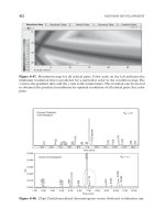
QT-RR plane. Figure 3.7 illustrates this point, with each of the central contours
indicating a response of either tachycardia (RT) and bradycardia (RB) or normal
resting. From the top right of each contour, moving counterclockwise (or anticlock-
wise); as the heart rate increases (the RR interval drops) the QT interval remains
constant for a few beats, and then begins to shorten, approximately in an inverse

square manner. When the heart rate drops (RR interval lengthens) a similar time
delay is observed before the QT interval begins to lengthen and the subject returns
to approximately the original point in the QT-RR phase plane. The difference be-
tween the two trajectories (caused by RR acceleration and deceleration) is the QT
hysteresis, and depends not only on the individual’s physiological condition, but
also on the specific activity in the ANS. Although the central contour defines the
limits of normality for a resting subject, active subjects exhibit an extended QT-RR
contour. The 95% limits of normal activity are defined by the large, asymmetric
dotted contour, and activity outside of this region can be considered abnormal.
The standard QT-RR relationship for low heart rates (defined by the Fridericia
correction factor QTc = QT/RR
1/3
) is shown by the line cutting the phase plane
from lower left to upper right. It can be seen that this factor, when applied to
the resting QT-RR interval relationship, overcorrects the dynamic responses in the
normal range (illustrated by the striped area above the correction line and below
the normal dynamic range) or underestimates QT prolongation at low heart rates
6.
Many QT correction factors have been considered that improve upon Bazett’s formula (QTc = QT/
√
RR),
including linear regression fitting (QTc = QT + 0.154(1 −RR)), which works well at high heart rates, and
the Fridericia correction (QTc = QT/RR
1/3
), which works well at low heart rates.
P1: Shashi
August 24, 2006 11:39 Chan-Horizon Azuaje˙Book
66 ECG Statistics, Noise, Artifacts, and Missing Data
Figure 3.7 Normal dynamic QT-RR interval relationship (dotted-line forming asymmetric contour)
encompasses autonomic reflex responses such as tachycardia (RT) and bradycardia (RB) with hys-

teresis. The statistical outer boundary of the normal contour is defined as the upper 95% confidence
bounds. The Fridericia correction factor applied to the resting QT-RR interval relationship overcor-
rects dynamic responses in the normal range (striped area above correction line and below 95%
confidence bounds) or underestimates QT prolongation at slow heart rates (shaded area above 95%
confidence bounds but below Fridericia correction). QT prolongation of undefined arrhythmogenic
risk (dark shaded area) occurs when exceeding the 95% confidence bounds of QT intervals during
unstressed autonomic influence. (From: [21].
c
 2005 ASPET: American Society for Pharmacology
and Experimental Therapeutics. Reprinted with permission.)
(shaded area above normal range but below Fridericia correction) [21]. Abnormal
QT prolongation is illustrated by the upper dark shaded area, and is defined to be
when the QT-RR vector exceeds the 95% normal boundary (dotted line) during
unstressed autonomic influence [21].
Another, more recently documented heart rate-related hysteresis is that of ST/HR
[22], which is a measure of the ischemic reaction of the heart to exercise. If ST de-
pression is plotted vertically so that negative values represent ST elevation, and
heart rate is plotted along the horizontal axis typical ST/HR diagrams for a clin-
ically normal subject display a negative hysteresis in ST depression against HR,
(a clockwise hysteresis loop in the ST-HR phase plane during postexercise recovery).
Coronary artery disease patients, on the other hand, display a positive hysteresis
in ST depression against HR (a counterclockwise movement in the hysteresis loop
during recovery) [23].
It is also known that the PR interval changes with heart rate, exhibiting a
(mostly) respiration-modulated dynamic, similar to (but not as strong as) the modu-
lation observed in the associated RR interval sequence [24]. This activity is described
in more detail in Section 3.7.
3.4.2 Arrhythmias
The normal nonstationary changes are induced, in part, by changes in the sympa-
thetic and parasympathetic branches of the autonomic nervous system. However,

P1: Shashi
August 24, 2006 11:39 Chan-Horizon Azuaje˙Book
3.5 Arrhythmia Detection 67
sudden (abnormal) changes in the ECG can occur as a result of malfunctions in the
normal conduction pathways of the heart. These disturbances manifest on the ECG
as, sometimes subtle, and sometimes gross distortions of the normal beat (depending
on the observation lead or the physiological origin of the abnormality). Such beats
are traditionally labeled by their etiology, into ventricular beats, supraventricular
and atrial.
7
Since ventricular beats are due to the excitation of the ventricles before the atria,
the P wave is absent or obscured. The QRS complex also broadens significantly since
conduction through the myocardium is consequently slowed (see Chapter 1). The
overall amplitude and duration (energy) of such a beat is thus generally higher. QRS
detectors can easily pick up such high energy beats and the distinct differences in
morphology make classifying such beats a fairly straightforward task. Furthermore,
ventricular beats usually occur much earlier or later than one would expect for a
normal sinus beat and are therefore known as VEBs, ventricular ectopic beats (from
the Greek, meaning out of place).
Abnormal atrial beats exhibit more subtle changes in morphology than ventric-
ular beats, often resulting in a reduced or absent P wave. The significant changes for
an atrial beat come from the differences in interbeat timings (see Section 3.2.2). Un-
fortunately, from a classification point of view, abnormal beats are sometimes more
frequent when artifact increases (such as during stress tests). Furthermore, artifacts
can often resemble abnormal beats, and therefore extra information from multiple
leads and beat context are often required to make an accurate classification.
3.5 Arrhythmia Detection
If conduction abnormalities are transient, then an abnormal beat manifests. If con-
duction problems persist, then the abnormal morphology repeats and an arrhythmia
is manifest, or the ECG degenerates into an almost unrecognizable pattern. There

are three general approaches to arrhythmia analysis. One method is to perform QRS
detection and beat classification, labeling an arrhythmia as a quorum of a series of
beats of a particular type. The common alternative approach is to analyze a section
of the ECG that spans several beat intervals, calculate a statistic (such as variance
or a ratio of power at different frequencies) on which the arrhythmia classifica-
tion is performed. A third option is to construct a model of the expected dynamics
for different rhythms and compare the observed signal (or derived features) to this
model. Such model-based approaches can be divided down into ECG-based meth-
ods or RR interval statistics-based methods. Linear ECG-modeling techniques [26]
are essentially equivalent to spectral analysis. Nonlinear state-space model recon-
structions have also been used [27], but with varying results. This may be partly due
to the sensitivity of nonlinear metrics to noise. See Chapter 6 for a more detailed
description of this technique together with a discussion of the problems associated
with applying nonlinear techniques to noisy data.
7.
The table in [25], which lists all the beat classifications labeled in the PhysioNet databases [2] together with
their alphanumeric labels, provides an excellent detailed list of beat types and rhythms.
P1: Shashi
August 24, 2006 11:39 Chan-Horizon Azuaje˙Book
68 ECG Statistics, Noise, Artifacts, and Missing Data
3.5.1 Arrhythmia Classification from Beat Typing
A run of abnormal beats can be classified as an arrhythmia. Therefore, as long as
consistent fiducial points can be located on a series of beats, simple postprocessing
of a beat classifier’s output together with a threshold on the heart rate can be
sufficient for correctly identifying many arrhythmias. For example, supraventricular
tachycardia is the sustained presence of supraventricular ectopic beats, at a rate over
100 bpm. Many more complex classification schemes have been proposed, including
the use of principal component analysis [28, 29] (see Chapters 9 and 10) hidden
Markov models [30], interlead comparisons [31], cluster analysis [32], and a variety
of supervised and unsupervised neural learning techniques [33–35]. Further details

of the latter category can be found in Chapters 12 and 13.
3.5.2 Arrhythmia Classification from Power-Frequency Analysis
Sometimes there is no consistently identifiable fiducial point in the ECG, and anal-
ysis of the normal clinical features is not possible. In such cases, it is usual to
exploit the changes in frequency characteristics that are present during arrhyth-
mias [36, 37]. More recently, joint time-frequency analysis techniques have been
applied [38–40], to take advantage of the nonstationary nature of the cardiac cycle.
Other interesting methods that make use of interchannel correlation techniques
have been proposed [31], but results from using a decision tree and linear classi-
fier on just three AR coefficients (effectively performing a multiple frequency band
thresholding) give some of the most promising results. Dingfei et al. [26] report clas-
sification performance statistics (sensitivity, specificity) on the MIT-BIH database [2]
of 93.2%, 94.4% for sinus rhythm, 100%, 96.2% for superventricular tachycardia,
97.7%, 98.6% for VT, and 98.6%, 97.7% for VFIB. They also report classification
statistics (sensitivity, specificity) of 96.4%, 96.7% for atrial premature contrac-
tions (APCs), and 94.8%, 96.8% for premature ventricular contractions (PVCs).
8
Sensitivity and specificity figures in the mid to upper 90s can be considered state
of the art. However, these results pertain to only one database and the (sensitive)
window size is prechosen based upon the prior expectation of the rhythm. Despite
this, this approach is extremely promising, and may be improved by developing a
method for adapting the window size and/or using a nonlinear classifier such as a
neural network.
3.5.3 Arrhythmia Classification from Beat-to-Beat Statistics
Zeng and Glass [8] described a model for AV node conduction which was able to
accurately model many observations of the statistical distribution of the beat-to-beat
intervals during atrial arrhythmias (see Chapter 4 for a more details on this model).
This model-based approach was further extended in [41] to produce a method of
classifying beats based upon their statistical distribution. Later, Schulte-Frohlinde
et al. [42] produced a variant of this technique that includes a dimension of time

and allows the researcher to observe the temporal statistical changes. Software for
this technique (known as heartprints) is freely available from [43].
More recent algorithms have attempted to combine both the spectral char-
acteristics and time domain features of the ECG (including RR intervals) [44].
8.
Sometimes called VPCs (ventricular premature contractions).
P1: Shashi
August 24, 2006 11:39 Chan-Horizon Azuaje˙Book
3.6 Noise and Artifact in the ECG 69
The integration of such techniques can help improve arrhythmia classification, but
only if the learning set is expanded in size and complexity in a manner that is
sufficient to provide enough training examples to account for the increased dimen-
sionality of the input feature space. See Chapters 12 and 13 for further discussions
of training, test, and validation data sets.
3.6 Noise and Artifact in the ECG
3.6.1 Noise and Artifact Sources
Unfortunately, the ECG is often contaminated by noise and artifacts
9
that can be
within the frequency band of interest and can manifest with similar morphologies
as the ECG itself. Broadly speaking, ECG contaminants can be classified as [45]:
1. Power line interference: 50 ±0.2 Hz mains noise (or 60 Hz in many data
sets
10
) with an amplitude of up to 50% of full scale deflection (FSD), the
peak-to-peak ECG amplitude;
2. Electrode pop or contact noise: Loss of contact between the electrode and the
skin manifesting as sharp changes with saturation at FSD levels for periods
of around 1 second on the ECG (usually due to an electrode being nearly or
completely pulled off);

3. Patient–electrode motion artifacts: Movement of the electrode away from
the contact area on the skin, leading to variations in the impedance between
the electrode and skin causing potential variations in the ECG and usually
manifesting themselves as rapid (but continuous) baseline jumps or complete
saturation for up to 0.5 second;
4. Electromyographic (EMG) noise: Electrical activity due to muscle contrac-
tions lasting around 50 ms between dc and 10,000 Hz with an average
amplitude of 10% FSD level;
5. Baseline drift: Usually from respiration with an amplitude of around 15%
FSD at frequencies drifting between 0.15 and 0.3 Hz;
6. Data collecting device noise: Artifacts generated by the signal processing
hardware, such as signal saturation;
7. Electrosurgical noise: Noise generated by other medical equipment present
in the patient care environment at frequencies between 100 kHz and 1 MHz,
lasting for approximately 1 and 10 seconds;
8. Quantization noise and aliasing;
9. Signal processing artifacts (e.g., Gibbs oscillations).
Although each of these contaminants can be reduced by judicious use of hard-
ware and experimental setup, it is impossible to remove all contaminants. There-
fore, it is important to quantify the nature of the noise in a particular data set and
9.
It should be noted that the terms noise and artifact are often used interchangeably. In this book artifact
is used to indicate the presence of a transient interruption (such as electrode motion) and noise is used to
describe a persistent contaminant (such as mains interference).
10.
Including recordings made in North and Central America, western Japan, South Korea, Taiwan, Liberia,
Saudi Arabia, and parts of the Caribbean, South America, and some South Pacific islands.
P1: Shashi
August 24, 2006 11:39 Chan-Horizon Azuaje˙Book
70 ECG Statistics, Noise, Artifacts, and Missing Data

choose an appropriate algorithm suited to the contaminants as well as the intended
application.
3.6.2 Measuring Noise in the ECG
The ECG contains very distinctive features, and automatic identification of these
features is, to some extent, a tractable problem. However, quantifying the nonsignal
(noise) element in the ECG is not as straightforward. This is partially due to the
fact that there are so many different types of noises and artifacts (see above) that
can occur simultaneously, and partially because these noises and artifacts are often
transient, and largely unpredictable in terms of their onset and duration. Standard
measures of noise-power assume stationarity in the dynamics and coloration of the
noise. These include:
•
Route mean square (RMS) power in the isoelectric region;
•
Ratio of the R-peak amplitude to the noise amplitude in the isoelectric region;
•
Crest factor / peak-to-RMS ratio (the ratio of the peak value of a signal to its
RMS value);
•
Ratio between in-band (5 to 40 Hz) and out-of-band spectral power;
•
Power in the residual after a filtering process.
Except for (16.
˙
6, 50, or 60 Hz) mains interference and sudden abrupt baseline
changes, the assumption that most noise is Gaussian in nature is approximately
correct (due to the central limit theorem). However, the coloration of the noise
can significantly affect any interpretation of the value of the noise power, since the
more colored a signal is, the larger the amplitude for a given power. This means
that a signal-to-noise ratio (SNR) for a brown noise contaminated ECG (such as

movement artifact) equates to a much cleaner ECG than the same SNR for an ECG
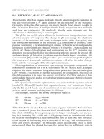
contaminated by pink noise (typical for observation noise). Figure 3.8 illustrates
this point by comparing a zero-mean unit-variance clean ECG (upper plot) with the
same signal with additive noise of decreasing coloration (lower autocorrelation).
In each case, the noise is set to be zero-mean with unit variance, and therefore has
the same power as the ECG (SNR = 1). Note that the whiter the noise, the more
significant the distortion for a given SNR. It is obvious that ECG analysis algorithms
will perform differently on each of these signals, and therefore it is important to
record the coloration of the noise in the signal as well as the SNR.
Determining the color of the noise in the ECG is a two-stage process which first
involves locating and removing the P-QRS-T features. Moody et al. [28, 29] have
shown that the QRS complex can be encoded in the first five principal components
(PCs). Therefore, a good approximate method for removing the signal component
from an ECG is to use all but the first five PCs to reconstruct the ECG. Principal
component analysis (PCA) involves the projection of N-dimensional data onto a
set of N orthogonal axes that represent the maximum directions of variance in the
data. If the data can be well represented by such a projection, the p axes along
which the variance is largest are good descriptors of the data. The N − p remaining
components are therefore projections of the noise. A more in-depth analysis of PCA
can be found in Chapters 5 and 9.
P1: Shashi
August 24, 2006 11:39 Chan-Horizon Azuaje˙Book
3.7 Heart Rate Variability 71
Figure 3.8 Zero-mean unit-variance clean ECG with additive brown, pink, and white noise (also
zero-mean and unit-variance, and hence SNR = 1 in all cases).
Practically, this involves segmenting each beat in the given analysis window
11
such that the start of each P wave and the end of each T wave (or U wave if present)
are captured in each segmentation with m-samples. The N beats are then aligned so
that they form an N×m matrix denoted, X. If singular value decomposition (SVD)

is then performed to determine the PCs, the five most significant components are
discarded (by setting the corresponding eigenvalues to zero), and the SVD inverted,
X becomes a matrix of only noise. The data can then be transformed back into a
1-D signal using the original segmentation indices.
The second stage involves calculating the log power-spectrum of this noise signal
and determine its slope. The resultant spectrum has a 1/f
β
form. That is, the slope
β determines the color of the signal with the higher the value of β, the higher the
auto-correlation. If β = 0, the signal is white (since the spectrum is flat) and is
completely uncorrelated. If β = 1, the spectrum has a 1/ f spectrum and is known
as pink noise, typical of the observation noise on the ECG. Electrode movement
noise has a Brownian motion-like form (with β = 2), and is therefore known as
brown noise.
3.7 Heart Rate Variability
The baseline variability of the heart rate time series is determined by many factors
including age, gender, activity, medications, and health [46]. However, not only
11.
The window must contain at least five beats, and preferably at least 30 to capture respiration and ANS-
induced changes in the ECG morphology; see Section 3.3.
P1: Shashi
August 24, 2006 11:39 Chan-Horizon Azuaje˙Book
72 ECG Statistics, Noise, Artifacts, and Missing Data
does the mean beat-to-beat interval (the heart rate) change on many scales, but the
variance of this sequence of each heartbeat interval does so too. On the shortest
scale, the time between each heartbeat is irregular (unless the heart is paced by an
artificial electrical source such as a pacemaker, or a patient is in a coma). These short-
term oscillations reflect changes in the relative balance between the sympathetic and
parasympathetic branches of the ANS, the sympathovagal balance. This heart rate
irregularity is a well-studied effect known as heart rate variability (HRV) [47].

HRV metric values are often considered to reflect the competing actions of these
different branches of the ANS on the sinoatrial (SA) node.
12
Therefore, RR intervals
associated with abnormal beats (that do not originate from the SA node) should
not be included in a HRV metric calculation and the series of consecutive normal-
to-normal (NN) beat intervals should be analyzed.
13
It is important to note that, the fiducial marker of each beat should be the onset
of the P wave, since this is a more accurate marker than the R peak of the SA node
stimulation (atrial depolarization onset) for each beat. Unfortunately, the P wave is
usually a low-amplitude wave and is therefore often difficult to detect. Conversely,
the R wave is easy to detect and label with a fiducial point. The exact location of this
marker is usually defined to be either the highest (or lowest) point, the QRS onset,
or the center of mass of the QRS complex. Furthermore, the competing effects of
the ANS branches lead to subtle changes in the features within the heartbeat. For
instance, a sympathetic innervation of the SA node (from exercise, for example) will
lead to an increased local heart rate, and an associated shortening of the PR interval
[10], QT interval [21], QRS width [48], and T wave [18]. Since the magnitude of
the beat-to-beat modulation of the PR interval is correlated with, and much less
significant than that of the RR interval [10, 49], and the R peak is well defined
and easy to locate, many researchers choose to analyze only the RR tachogram
(of normal intervals). It is unclear to what extent the differences in fiducial point
location affects measures of HRV, but the sensitivity of the spectral HRV metrics to
sampling frequencies below 1 kHz indicates that even small differences may have a
significant effect for such metrics under certain circumstances [50].
If we record a typical RR tachogram over at least 5 minutes, and calculate
the power spectral density,
14
then two dominant peaks are sometimes observable;

one in the low frequency (LF) range (0.015 < f < 0.15 Hz) and one in the high
frequency (HF) region (0.15 ≤ f ≤ 0.4 Hz). In general, the activity in the HF band
is thought to be due mainly to parasympathetic activity at the sinoatrial node. Since
respiration is a parasympathetically mediated activity (through the vagal nerve), a
peak corresponding to the rate of respiration can often be observed in this frequency
band (i.e., RSA). However, not all the parasympathetic activity is due to respiration.
Furthermore, the respiratory rate may drop below the (generally accepted) lower
bound of the HF region and therefore confound measures in the LF region. The LF
region is generally thought to reflect sympathetically mediated activity
15
such as
12.
See Chapter 1 for more details.
13.
The temporal sequence of events is therefore known as the NN tachogram, or more frequently the RR
tachogram (to indicate that each point is between each normal R peak).
14.
Care must be taken at this point, as the time series is unevenly sampled; see section 3.7.2.
15.
Although there is some evidence to show that this distinction does not always hold [46].
P1: Shashi
August 24, 2006 11:39 Chan-Horizon Azuaje˙Book
3.7 Heart Rate Variability 73
blood pressure-related phenomena. Activity in bands lower than the LF region are
less well understood but seem to be related to myogenic activity, physical activity,
and circadian variations. Note also that these frequency bands are on some level
quite ad hoc and should not be taken as the exact limits on different mechanisms
within the ANS; there are many studies that have used variants of these limits with
practical results.
Many metrics for evaluating HRV have been described in the literature, together

with their varying successes for discerning particular clinical problems. In general,
HRV metrics can be broken down into either statistical time-based metrics (e.g.,
variance), or frequency-based metrics that evaluate power, or ratios of power, in
certain spectral bands. Furthermore, most metrics are calculated either on a short
time scale (often about 5 minutes) or over extremely long periods of time (usually
24 hours). The following two subsections give a brief overview of many of the
common metrics. A more detailed analysis of these techniques can be found in the
references cited therein. A comprehensive survey of the field of HRV was conducted
by Malik et al. [46, 51] in 1995, and although much of the material remains relevant,
some recent notable recent developments are included below, which help clarify
some of the problems noted in the book. In particular, the sensitivity (and lack of
specificity) of HRV metrics in many experiments has been shown to be partly due
to activity-related changes [52] and the widespread use of resampling [53]. These
issues, together with some more recent metrics, will now be explored.
3.7.1 Time Domain and Distribution Statistics
Time domain statistics are generally calculated on RR intervals without resampling,
and are therefore robust to aggressive data removal (of artifacts and ectopic beats;
see Section 3.7.6). An excellent review of conventional time domain statistics can
be found in [46, 51]. One recently revisited time domain metric is the pNN50; the
percentage of adjacent NN intervals differing by more than 50 ms over an entire 24-
hour ECG recording. Mietus et al. [54] studied the generalization of this technique;
the pNNx— the percentage of NN intervals in a 24-hour time series differing by
more than xms (4 ≤ x ≤ 100). They found that enhanced discrimination between
a variety of normal and pathological conditions is possible by using a value of x
as low as 20 ms or less, rather than the standard 50 ms threshold. This tool, and
many of the standard HRV tools, are freely available from PhysioNet [2]. This work
can be considered similar to recent work by Grogan et al. [55], who analyzed the
predictive power of different bins in a smoothed RR interval histogram and termed
the metric cardiac volatility. Histogram bins were isolated that were more predictive
of deterioration in the ICU than conventional metrics, despite the fact that the data

was averaged over many seconds. These results indicate that only certain frequencies
of cardiac variability may be indicative of certain conditions, and that conventional
techniques may be including confounding factors, or simply noise, into the metric
and diminishing the metric’s predictive power.
In Malik and Camm’s collection of essays on HRV [51], metrics that involve a
quantification of the probability distribution function of the NN intervals over a
long period of time (such as the TINN, the “triangular index”), were referred to as
geometrical indices. In essence, these metrics are simply an attempt at calculating
P1: Shashi
August 24, 2006 11:39 Chan-Horizon Azuaje˙Book
74 ECG Statistics, Noise, Artifacts, and Missing Data
robust approximations of the higher order statistics. However, the higher the
moment, the more sensitive it is to outliers and artifacts, and therefore, such “geo-
metrical” techniques have faded from the literature.
The fourth moment, kurtosis, measures how peaked or flat a distribution is,
relative to a Gaussian (see Chapter 5), in a similar manner to the TINN. Approx-
imations to kurtosis often involve entropy, a much more robust measure of non-
Gaussianity. (A key result of information theory is that, for a set of independent
sources, with the same variance, a Gaussian distribution has the highest entropy,
of all the signals.) It is not surprising then, that entropy-based HRV measures are
more frequently employed that kurtosis.
The third moment of a distribution, skewness, quantifies the asymmetry of a
distribution and has therefore been applied to patients in which sudden acceler-
ations in heart rate, followed by longer decelerations, are indicative of a clinical
problem. In general, the RR interval sequence accelerates much more quickly than
it decelerates.
16
Griffin and Moorman [56] have shown that a small difference in
skewness (0.59 ±0.10 for sepsis and 0.51 ±0.012 for sepsis-like illness, compared
with −0.10 ± 0.13 for controls) can be an early indicator (up to 6 hours) of an

upcoming abrupt deterioration in newborn infants.
3.7.2 Frequency Domain HRV Analysis
Heart rate changes occur on a wide range of time scales. Millisecond sympathetic
changes stimulated by exercise cause an immediate increase in HR resulting in
a lower long-term baseline HR and increased HRV over a period of weeks and
months. Similarly, a sudden increase in blood pressure (due to an embolism, for
example) will lead to a sudden semipermanent increase in HR. However, over many
months the baroreceptors will reset their operating range to cause a drop in baseline
HR and blood pressure (BP). In order to better understand the contributing factors
to HRV and the time scales over which they affect the heart, it is useful to consider
the RR tachogram in the frequency domain.
3.7.3 Long-Term Components
In general, the spectral power in the RR tachogram is broken down into four bands
[46]:
1. Ultra low frequency (ULF): 0.0001 Hz ≥ ULF < 0.003 Hz;
2. Very low frequency (VLF): 0.003 Hz ≥ VLF < 0.04 Hz;
3. Low frequency (LF): 0.04 Hz ≥ LF < 0.15 Hz;
4. High frequency (HF): 0.15 Hz ≥ HF < 0.4 Hz.
Other upper- and lower-frequency bands are sometimes used. Frequency domain
HRV metrics are then formed by summing the power in these bands, taking ratios,
16.
Parasympathetic withdrawal is rapid, but is damped out by either parasympathetic activation or a much
slower sympathetic withdrawal.
P1: Shashi
August 24, 2006 11:39 Chan-Horizon Azuaje˙Book
3.7 Heart Rate Variability 75
Figure 3.9 Typical periodogram of a 24-hour RR tachogram where power is plotted vertically and
the frequency plotted horizontally on a log scale. Note that the gradient β of the log −log plot is
only meaningful for the longer scales. (After: [46].)
or calculating the slope,

17
β,ofthelog − log power spectrum; see Figure 3.9.
The motivation for splitting the spectrum into these frequency bands lies in the
belief that the distinct biological regulatory mechanisms that contribute to HRV act
at frequencies that are confined (approximately) within these bands. Fluctuations
below 0.04 Hz in the VLF and ULF bands are thought to be due to long-term
regulatory mechanisms such as the thermoregulatory system, the reninangiotensin
system (related to blood pressure and other chemical regulatory factors), and other
humoral factors [57]. In 1998 Taylor et al. [58] showed that the VLF fluctuations
appear to depend primarily on the parasympathetic outflow. In 1999 Serrador et al.
[59] demonstrated that the ULF band appears to be dominated by contributions
from physical activity and that HRV in this band tends to increase during exercise.
They therefore assert that any study that assesses HRV using data (even partially)
from this frequency band should always include an indication of physical activity
patterns. However, the effect of physical (and moreover, mental) activity on HRV is
so significant that it has been suggested that controlling for activity for all metrics
is extremely important [52].
Since spectral analysis was first introduced into HRV analysis in the late 1960s
and early 1970s [60, 61], a large body of literature has arisen concerning this topic.
17.
In the HRV literature, this slope is sometimes denoted by α.
P1: Shashi
August 24, 2006 11:39 Chan-Horizon Azuaje˙Book
76 ECG Statistics, Noise, Artifacts, and Missing Data
In 1993, the U.S. Food and Drug Administration (FDA) withdrew its support of
HRV as a useful clinical parameter due to a lack of consensus on the efficacy and
applicability of HRV in the literature [62]. Although the Task Force of the European
Society of Cardiology and the North American Society of Pacing Electrophysiology
[46] provided an extensive overview of HRV estimation methods and the associated
experimental protocols in 1996, the FDA has been reluctant to approve medical

devices that calculate HRV unless the results are not explicitly used to make a
specific medical diagnosis (e.g., see [63]). Furthermore, the clinical utility of HRV
analysis (together with FDA approval) has only been demonstrated in very limited
circumstances, where the patient undergoes specific tests (such as paced breathing
or the Valsalva Maneuver) and the data are analyzed off-line by experts [64].
Almost all spectral analysis of the RR tachogram has been performed using
some variant of autoregressive (AR) spectral estimation
18
or the FFT [46], which
implicitly requires stationarity and regularly spaced samples. It should also be noted
that most spectral estimation techniques such as the FFT require a windowing tech-
nique (e.g., the hamming window
19
), which leads to an implicit nonlinear distortion
of the RR tachogram, since the value of the RR tachogram is explicitly joined to
the time stamp.
20
To mitigate for nonstationarities, linear and polynomial detrending is often
employed, despite the lack of any real justification for this procedure. Furthermore,
since the time stamps of each RR interval are related to the previous RR interval,
the RR tachogram is inherently unevenly (or irregularly) sampled. Therefore, when
using the FFT, the RR tachogram must either be represented in terms of power
per cycle per beat (which varies based upon the local heart rate, and it is therefore
extremely difficult, if not impossible, to compare one calculation with another) or
a resampling method is required to make the time series evenly sampled.
Common resampling schemes involve either linear or cubic spline interpola-
tive resampling. Resampling frequencies between 2 and 10 Hz have been used,
but as long as the Nyquist criterion is satisfied, the resampling rate does not ap-
pear to have a serious effect on the FFT-based metrics [53]. However, experiments
on both artificial and real data reveal that such processes overestimate the total

power in the LF and HF bands [53] (although the increase is marginal for the cubic
18.
Clayton et al. [65] have demonstrated that FFT and AR methods can provide a comparable measure of the
low-frequency LF and high-frequency HF metrics on linearly resampled 5-minute RR tachograms across
a patient population with a wide variety of ages and medical conditions (ranging from heart transplant
patients who have the lowest known HRV to normals who often exhibit the highest overall HRV). AR
models are particularly good at identifying line spectra and are therefore perhaps not an appropriate
technique for analyzing HRV activity. Furthermore, since the optimal AR model order is likely to change
based on the activity of the patient, AR spectral estimation techniques introduce an extra complication in
frequency-based HRV metric estimation. AR modeling techniques will therefore not be considered in this
chapter. As a final aside on AR analysis, it is interesting to note that measuring the width of a Poincar
´
e plot
is the same as treating the RR tachogram as an AR1 process and then estimating the process coefficient.
19.
In the seminal 1978 paper on spectral windowing [66], Harris demonstrated that a hamming window
(given by W(t
j
) = 0.54 − 0.46 cos(ωt
j
), [ j = 0, 1, 2, , N − 1]) provides an excellent performance for
FFT analysis in terms of spectral leakage, side lobe amplitude, and width of the central peak (as well as a
rapid computational time).
20.
However, the window choice does not appear to affect the HRV spectral estimates significantly for RR
interval variability.
P1: Shashi
August 24, 2006 11:39 Chan-Horizon Azuaje˙Book
3.7 Heart Rate Variability 77
spline resampling if the RR tachogram is smoothly varying and there are no missing

or removed data points due to ectopy or artifact; see Section 3.7.6). The FFT over-
estimates the
LF
HF
-ratio by about 50% with linear resampling and by approximately
10% with cubic spline resampling [53]. This error can be greater than the difference
in the
LF
HF
-ratio between patient categories and is therefore extremely significant (see
Section 3.7.7). One method for reducing (and almost entirely removing) this distor-
tion is to use the Lomb-Scargle periodogram (LSP) [67–71], a method of spectral
estimation which requires no explicit data replacement (nor assumes any underly-
ing model) and calculates the PSD from only the known (observed) values in a time
series.
3.7.4 The Lomb-Scargle Periodogram
Consider a physical variable X measured at a set of times t
j
where the sampling is
at equal times (t = t
j+1
− t
j
= constant) from a stochastic process. The resulting
time series data, {X(t
j
)} (i = 1, 2, , N), are assumed to be the sum of a signal
X
s
and random observational errors,

21
R;
X
j
= X(t
j
) = X
s
(t
j
) + R(t
j
) (3.2)
Furthermore, it is assumed that the signal is periodic, that the errors at different
times are independent (R(t
j
) = f ( R(t
k
)) for j = k) and that R(t
j
) is normally
distributed with zero mean and constant variance, σ
2
.
The N-point discrete Fourier transform (DFT) of this sequence is
FT
X
(ω) =
N−1


j=0
X(t
j
)e
−iωt
j
(3.3)
(ω
n
= 2π f
n
, n = 1, 2, , N) and the power spectral density estimate is therefore
given by the standard method for calculating a periodogram:
P
X
(ω) =
1
N
N−1

j=0


X(t
j
)e
−iωt
j



2
(3.4)
Now consider arbitrary t
j
’s or uneven sampling (t = t
j+1
− t
j
=constant) and a
generalization of the N-point DFT [68]:
F :T
X
(ω) =

N
2

1
2
N−1

j=0
X(t
j
)[Acos(ωt
j
) −iBsin(ωt
j
)] (3.5)
where i =

√
−1, j is the summation index, and A and B are as yet unspecified
functions of the angular frequency ω. This angular frequency may depend on the
21.
Due to the additive nature of the signal and the errors in measuring it, the errors are often referred to as
noise.
P1: Shashi
August 24, 2006 11:39 Chan-Horizon Azuaje˙Book
78 ECG Statistics, Noise, Artifacts, and Missing Data
vector of sample times, {t
j
}, but not on the data, {X(t
j
)}, nor on the summation
index j. The corresponding (normalized) periodogram is then
P
X
(ω) =
1
N
|FT
X
(ω)|
2
=
A
2
2




j
X(t
j
) cos(ωt
j
)


2
+
B
2
2



j
X(t
j
) sin(ωt
j
)


2
(3.6)
If A = B =

2

N

1
2
, (3.5) and (3.6) reduce to the classical definitions [(3.3) and
(3.4)] For even sampling (t = constant) FT
X
reduces to the DFT and in the limit
t → 0, N →∞, it is proportional to the Fourier transform. Scargle [68] shows
how (3.6) is not unique and further conditions must be imposed in order to derive
the corrected expression for the LSP:
P
N
(ω) ≡
1
2σ
2







j
(x
j
− x) cos(ω(t
j
− τ ))


2

j
cos
2
(ω(t
j
− τ ))
+


j
(x
j
− x) sin(ω(t
j
− τ ))

2

j
sin
2
(ω(t
j
− τ ))






(3.7)
where τ ≡ tan
−1


j
sin(2ωt
j
)
2ω

j
cos(2ωt
j
)

. τ is an offset that makes P
N
(ω) completely in-
dependent of shifting all the t
j
’s by any constant. This choice of offset makes (3.7)
exactly the solution that one would obtain if the harmonic content of a data set,
at a given frequency ω, was estimated by linear least-squares fitting to the model
x(t) = Acos(ωt) + B sin(ωt). Thus, the LSP weights the data on a per-point basis
instead of weighting the data on a per-time interval basis. Note that in the evenly
sampled limit (t = t
j+1

−t
j
= constant), (3.7) reduces to the classical periodogram
definition [67]. See [67–72] for mathematical derivations and further details. C and
Matlab code (lomb.c and lomb.m) for this routine are available from PhysioNet
[2, 70] and the accompanying book Web site [73]. The well-known numerical
computation library Numerical Recipes in C [74] also includes a rapid FFT-based
method for computing the LSP, which claims not to use interpolation (rather
extirpolation), but an implicit interpolation is still performed in the Fourier do-
main. Other methods for performing spectral estimation from irregularly sampled
data do exist and include the min-max interpolation method [75] and the well-
known geostatistical technique of krigging
22
[76]. The closely related fields of miss-
ing data imputation [77] and latent variable discovery [78] are also appropriate
routes for dealing with missing data. However, the LSP appears to be sufficient for
HRV analysis, even with a low SNR [53].
22.
Instead of weighting nearby data points by some power of their inverted distance, krigging uses the spatial
correlation structure of the data to determine the weighting values.
P1: Shashi
August 24, 2006 11:39 Chan-Horizon Azuaje˙Book
3.7 Heart Rate Variability 79
3.7.5 Information Limits and Background Noise
In order to choose a sensible window size, the requirement of stationarity must be
balanced against the time required to resolve the information present. The European
and North American Task Force on standards in HRV [46] suggests that the shortest
time period over which HRV metrics should be assessed is 5 minutes. As a result, the
lowest frequency that can be resolved is
1

300
≈ 0.003 Hz (just above the lower limit of
the VLF region). Such short segments can therefore only be used to evaluate metrics
involving the LF and HF bands. The upper frequency limit of the highest band for
HRV analysis is 0.4 Hz [51]. Since the average time interval for N points over a time
T is t
av
=
T
N
, then the average Nyquist frequency [68] is then f

c
=
1
2t
av
=
N
2T
.
Thus, a 5-minute window (T = 300) with the Nyquist constraint of
N
2T
≥ 0.4 for
resolving the upper frequency band of the HF region, leads to a lower limit on N
of 240 beats (an average heart rate of 48 bpm if all beats in a 5-minute segment
are used). Utilization of the LSP, therefore, reveals a theoretical lower information
threshold for accepting segments of an RR tachogram for spectral analysis in the
upper HF region. If RR intervals of at least 1.25 seconds (corresponding to an

instantaneous heart rate of HR
i
=
60
RR
i
= 48 bpm) exist within an RR tachogram,
then frequencies up to 0.4 Hz do exist. However, the accuracy of the estimates of
the higher frequencies is a function of the number of RR intervals that exist with
a value corresponding to this spectral region. Tachograms with no RR intervals
smaller than 1.25s (HR
i
< 48 bpm) can still be analyzed, but there is no power
contribution at 0.4 Hz.
This line of thought leads to an interesting viewpoint on traditional short-term
HRV spectral analysis; interpolation adds extra (erroneous) information into the
time series and pads the FFT (in the time domain), tricking the user into assuming
that there is a signal there, when really, there are simply not enough samples within
a given range to allow the detection of a signal (in a statistically significant sense).
Scargle [68] shows that at any particular frequency, f , and in the case of the null
hypothesis, P
X
(ω), has an exponential probability distribution with unit mean.
Therefore, the probability that P
X
(ω) will be between some positive value z and dz
is e
−z
dz, and hence, for a set of M independent frequencies, the probability that
none give values larger than z is (1 − e

−z
)
M
. The false alarm probability of the null
hypothesis is therefore
P(> z) ≡ 1 − (1 − e
−z
)
M
(3.8)
Equation (3.8) gives the significance level for any peak in the LSP, P
X
(ω) (a small
value, say, P < 0.05 indicates a highly significant periodic signal at a given fre-
quency). M can be determined by the number of frequencies sampled and the num-
ber of data points, N (see Press et al. [69]). It is therefore important to perform
this test on each periodogram before calculating a frequency-based HRV metric,
in order to check that there really are measurable frequencies that are not masked
by noise or nonstationarity. There is one further caveat: Fourier analysis assumes
that the signals at each frequency are independent. As we shall see in the next chap-
ter on modeling, this assumption may be approximately true at best, and in some
cases the coupling between different parts of the cardiovascular system may render
Fourier-based spectral estimation inapplicable.
P1: Shashi
August 24, 2006 11:39 Chan-Horizon Azuaje˙Book
80 ECG Statistics, Noise, Artifacts, and Missing Data
3.7.5.1 A Note on Spectral Leakage and Window Carpentry
The periodogram for unevenly spaced data allows two different forms of spectral
adjustment: the application of time-domain (data) windows through weighting the
signal at each point, and adjustment of the locations of the sampling times. The

time points control the power in the window function, which leaks to the Nyquist
frequency and beyond (the aliasing), while the weights control the side lobes. Since
the axes of the RR tachogram are intricately linked (one is the first difference of the
other), applying a windowing function to the amplitude of the data implicitly applies
a nonlinear stretching function to the sample points in time. For an evenly sampled
stationary signal, this distortion would affect all frequencies equally. Therefore,
the reductions in LF and HF power cancel when calculating the
LF
HF
-ratio. For an
irregularly sampled time series, the distortion will depend on the distribution of the
sampling irregularity. A windowing function is therefore generally not applied to
the irregularly sampled data. Distortion in the spectral estimate due to edge effects
will not result as long as the start and end point means and first derivatives do not
differ greatly [79].
3.7.6 The Effect of Ectopy and Artifact and How to Deal with It
To evaluate the effect of ectopy on HRV metrics, we can add artificial ectopic beats to
an RR tachogram using a simple procedure. Kamath et al. [80] define ectopic beats
(in terms of timing) as those which have intervals less than or equal to 80% of the
previous sinus cycle length. Each datum in the RR tachogram represents an interval
between two beats and the insertion of an ectopic beat therefore corresponds to the
replacement of two data points as follows. The nth and (n +1)th beats (where n is
chosen randomly) are replaced (respectively) by
RR

n
= γ RR
n−1
(3.9)
RR


n+1
= RR
n+1
+ RR
n
− RR

n
(3.10)
where the ectopic beat’s timing is the fraction, γ , of the previous RR interval (initially
0.8). Note that the ectopic beat must be introduced at random within the central
50% of the 5-minute window to avoid windowing effects. Table 3.2 illustrates
the effect of calculating the LF, HF, and
LF
HF
-ratio HRV metrics on an artificial
RR tachogram with a known
LF
HF
-ratio (0.64) for varying levels of ectopy (adapted
from [53]). Note that increasing levels of ectopy lead to an increase in HF power and
a reduction in LF power, significantly distorting the
LF
HF
-ratio (even for just one beat).
It is therefore obvious that ectopic beats must be removed from the RR tacho-
gram. In general, FFT-based techniques require the replacement of the removed beat
with a phantom beat at a location where one would have expected the beat to have
occurred if it was a sinus beat. Methods for performing phantom beat replacement

range from linear and cubic spline interpolation,
23
AR model prediction, segment
removal, and segment replacement.
23.
Confusingly, phantom beat replacement is generally referred to as interpolation. In this chapter, it is referred
to as phantom beat insertion, to distinguish it from the mathematical methods used to either place the
phantom beat, or resample the unevenly sampled tachogram.
P1: Shashi
August 24, 2006 11:39 Chan-Horizon Azuaje˙Book
3.7 Heart Rate Variability 81
Table 3.2 LSP Derived Frequency Metrics for Different
Magnitudes of Ectopy (γ )
Metric →
LF
HF
LF HF γ
Actual Value ↓
0.64 0.64 0.39 0.61
†
0.64 0.60 0.37 0.62 0.8
0.64 0.34 0.26 0.74 0.7
0.64 0.32 0.25 0.76 0.6
0.64 0.47 0.32 0.68 0.8
‡
†
indicates no ectopy is present.
‡ indicates two ectopic beats are present.
Source: [52].
Although more robust and promising model-based techniques have been used

[81], Lippman et al. [82] found that simply removing the signal around the ectopic
beat performed as well as these more complicated methods. Furthermore, resam-
pling the RR tachogram at a frequency ( f
s
) below the original ECG ( f
ecg
> f
s
) from
which it is derived effectively shifts the fiducial point by up to
1
2
(
1
f
s
−
1
f
ecg
)s. The
introduction of errors in HRV estimates due to low sampling rates is a well-known
problem, but the additive effect from resampling is underappreciated. If a patient is
suffering from low HRV (e.g., because they have recently undergone a heart trans-
plant or are in a state of coma) then the sampling frequency of the ECG must be
higher than normal. Merri et al. [83], and Abboud et al. [84] have shown that for
such patients a sampling rate of at least 1,000 Hz is required. Work by Clifford et
al. [85] and Ward et al. [50] demonstrate that a sampling frequency of 500 Hz or
greater is generally recommended (see Figure 4.9 and Section 4.3.2).
The obvious choice for spectral estimation for HRV is therefore the LSP, which

allows the removal of up to 20% of the data points in an RR tachogram without
introducing a significant error in an HRV metric [53]. Therefore, if no morpho-
logical ECG is available, and only the RR intervals are available, it is appropriate
to employ an aggressive beat removal scheme (removing any interval that changes
by more than 12.5% on the previous interval [86]) to ensure that ectopic beats are
not included in the calculation. Of course, since the ectopic beat causes a change in
conduction, and momentarily disturbs the sinus rhythm, it is inappropriate to in-
clude the intervals associated with the beats that directly follow an ectopic beat (see
Section 3.8.3.1) and therefore, all the affected beats should be removed at this non-
stationarity. As long as there is no significant change in the phase of the sinus rhythm
after the run of affected beats, then the LSP can be used without seriously affecting
the estimate. Otherwise, the time series should be segmented at the nonstationarity.
3.7.7 Choosing an Experimental Protocol: Activity-Related Changes
It is well known that clinical investigations should be controlled for drugs, age,
gender, and preexisting conditions. One further factor to consider is the activity
of the patient population group, for this may turn out to be the single largest
confounder of metrics, particularly in HRV studies. In fact, some HRV studies
may be doing little more than identifying the difference in activity between two
P1: Shashi
August 24, 2006 11:39 Chan-Horizon Azuaje˙Book
82 ECG Statistics, Noise, Artifacts, and Missing Data
patient groups, something that can be more easily achieved by methods such as
actigraphy, direct electrode noise analysis [87], or simply noting of the patient’s
activity using an empirical scale. Bernardi et al. [88] demonstrated that HRV in
conscious patients (as measured by the
LF
HF
-ratio) changes markedly depending on a
subject’s activity. Their analysis involved measuring the ECG, respiration, and blood
pressure of 12 healthy subjects, all aged around 29 years, for 5 minutes during a

series of simple physical (verbal) and mental activities. Despite the similarity in
subject physiology and physical activity (all remained in the supine position for at
least 20 minutes prior to, and during the recording), the day-time
LF
HF
-ratio had a
strong dependence on mental activity, ranging from 0.7 for controlled breathing to
3.6 for free talking. It may be argued that the changes in these values are simply an
effect of changing breathing patterns (that modify the HF component). However,
significant changes in both the LF component and blood pressure readings were also
observed, indicating that the feedback loop to the central nervous system (CNS)
was affected. The resultant change in HRV is therefore likely to be more than just
a respiratory phenomenon.
Differences in mental as well as physical activity should therefore be minimized
when comparing HRV metrics on an interpatient or intrapatient basis. Since it is
probably impossible to be sure whether or not even a willing subject is controlling
their thought processes for a few minutes (the shortest time window for traditional
HRV metrics [46]), this would imply that HRV is best monitored while the subject
is asleep, during which the level of mental activity can be more easily assessed.
Furthermore, artifact in the ECG is significantly reduced during sleep (because
there is less physical movement by the subject) and the variation in
LF
HF
-ratio with
respect to the mean value is reduced within a sleep state [52, 53, 72]. Sleep stages
usually last more than 5 minutes [89], which is larger than the minimum required
for spectral analysis of HRV [51]. Segmenting the RR time series according to sleep
state basis should therefore provide data segments of sufficient length with minimal
data corruption and departures from stationarity (which otherwise invalidate the
use of Fourier techniques).

The standard objective scale for CNS activity during sleep was defined by
Rechtschaffen and Kales [90], a set of heuristics known as the R&K rules. These
rules are based partially on the frequency content of the EEG, assessed by expert
observers over 30-second epochs. One of the five defined stages of sleep is termed
dream, or rapid eye movement (REM), sleep. Stages 1–4 (light to deep) are non-REM
(NREM) sleep, in which dreaming does not occur. NREM sleep can be further bro-
ken down into drowsy sleep (stage 1), light sleep, (stages 1 and 2), and deep sleep
(stages 3 and 4), or slow wave sleep (SWS). Healthy humans cycle through these
five sleep stages with a period of around 100 minutes, and each sleep stage can
last up to 20 minutes during which time the cardiovascular system undergoes few
changes, with the exception of brief arousals [89].
When loss of consciousness occurs, the parasympathetic nervous system begins
to dominate with an associated rise in HF and decrease in
LF
HF
-ratio. This trend
is more marked for deeper levels of sleep [91, 92]. PSDs calculated from 5 min-
utes of RR interval data during wakefulness and REM sleep reveal similar spectral
components and
LF
HF
-ratios [92]. However, stage 2 sleep and SWS sleep exhibit a
shift towards an increase in percentage contributions from the HF components
P1: Shashi
August 24, 2006 11:39 Chan-Horizon Azuaje˙Book
3.8 Dealing with Nonstationarities 83
Table 3.3
LF
HF
-Ratios During Wakefulness, NREM and REM Sleep

Activity → Awake REM NREM
Condition ↓ Sleep Sleep
Normal [92] N/A 2→2.5 0.5→1
Normal [46] 3.9 2.7 1.7
Normal [91] 4.0 ± 1.43.1 ± 0.71.2 ± 0.4
CNS Problem [93] N/A 3.5→5.5 2→3.5
Post-MI [91] 2.4 ± 0.78.9 ± 1.65.1 ± 1.4
Note: N/A = not available; Post-MI = a few days after myocardial infarction;
CNS = noncardiac related problem. Results quoted from [46, 91–93].
(above 0.15 Hz) with
LF
HF
-ratio values around 0.5 to 1 in NREM sleep and 2 to
2.5 in REM sleep [92]. In patients suffering from a simple CNS but noncardiac
related problem, Lavie et al. [93] found slightly elevated NREM
LF
HF
-ratio values
of between 2 and 3.5 and between 3.5 and 5.5 for REM sleep. Vanoli et al. [91]
report that myocardial infarction (MI) generally results in a raised overall
LF
HF
-ratio
during REM and NREM sleep with elevated LF and
LF
HF
-ratio (as high as 8.9) and
lower HF. Values for all subjects during wakefulness in these studies (2.4 to 4.0) lie
well within the range of values found during sleep (0.5 to 8.9) for the same patient
population (see Table 3.3). This demonstrates that comparisons of HRV between

subjects should be performed on a sleep-stage specific basis.
Recent studies [52, 53] have shown that the segmentation of the ECG into
sleep states and the comparison of HRV metrics between patients on a per-sleep
stage basis increases the sensitivity sufficiently to allow the separation of subtly
different patient groups (normals and sleep apneics
24
), as long as a suitable spectral
estimation technique (the LSP) is also employed. In particular, it was found that
deep sleep or SWS gave the lowest variance in the
LF
HF
-ratio both in an intrapatient
and interpatient basis, with the fewest artifacts, confirming that SWS is the most
stable of all the sleep stages. However, since certain populations do not experience
much SWS, it was found that REM sleep is an alternative (although slightly more
noisy) state in which to compare HRV metrics. Further large-scale studies are re-
quired to prove that sleep-based segmentation will actually provide patient-specific
assessments from HRV, although recent studies are promising.
3.8 Dealing with Nonstationarities
It should be noted at this point that all of the traditional HRV indices employ
techniques that assume (weak) stationarity in the data. If part of the data in the
window of analysis exhibits significant changes in the mean or variance over the
length of the window, the HRV estimation technique can no longer be trusted. A
cursory analysis of any real RR tachogram reveals that shifts in the mean or variance
are a frequent occurrence [94]. For this reason it is common practice to detrend the
signal by removing the linear or parabolic baseline trend from the window prior to
calculating a metric.
24.
Even when all data associated with the apneic episodes were excluded.
P1: Shashi

August 24, 2006 11:39 Chan-Horizon Azuaje˙Book
84 ECG Statistics, Noise, Artifacts, and Missing Data
However, this detrending does not remove any changes in variance over a sta-
tionarity change, nor any changes in the spectral distribution of component frequen-
cies. It is not only illogical to attempt to calculate a metric that assumes stationarity
over the window of interest in such circumstances, it is unclear what the meaning
of a metric taken over segments of differing autonomic tone could be. Moreover,
changes in stationarity of RR tachograms are often joined by transient sections of
heart rate overshoot and an accompanying increased probability of artifact on the
ECG (and hence missing data) [86, 95].
In this section we will explore a selection of methods for dealing with nonsta-
tionarities, including multiscale techniques, detrending, segmentation (both statis-
tically and from a clinical biological perspective), and the analysis of change points
themselves.
3.8.1 Nonstationary HRV Metrics and Fractal Scaling
Empirical analyses employing detrending techniques can lead to metrics that appear
to distinguish between certain patient populations. Such techniques include multi-
scale power analysis such as detrended fluctuation analysis (DFA) [96, 97]. Such
techniques aid in the quantification of long-range correlations in a time series, and
in particular, the fractal scaling of the RR tachogram. If a time series is self-similar
over many scales, then the log −log power-frequency spectrum will exhibit a 1/f
β
scaling, where β is the slope of the spectrum. For a white noise process the spectrum
is flat and β = 0. For pink noise processes, β = 1, and for Brownian processes,
β = 2. Black noise has β>2.
DFA is an alternative variance-based method for measuring the fractal scal-
ing of a time series. Consider an N-sample time series x
k
, which is integrated to
give a time series y

k
that is divided into boxes of equal length, m. In each box a
least squares line fit is performed on the data (to estimate the trend in that box).
The y coordinate of the straight line segments is denoted by y
(m)
k
. Next, the inte-
grated time series, y
k
, is detrended by subtracting the local trend, y
(m)
k
, in each box.
The root-mean-square fluctuation of this integrated and detrended time series is
calculated by
F (m) =




1
N

N

k=1

y
k
− y

(m)
k

2

(3.11)
This computation is repeated over all time scales (box sizes) to characterize the rela-
tionship between F (m), the average fluctuation, as a function of box size. Typically,
F (m) will increase with box size m. A linear relationship on a log−log plot indicates
the presence of power law (fractal) scaling. Under such conditions, the fluctuations
can be characterized by a scaling exponent α, the slope of the line relating log F (m)
to log m, that is, F(m) ∼ m
α
.
A direct link between DFA and conventional spectral analysis techniques and
other fractal dimension estimation techniques exists [98–101]. These techniques in-
clude semivariograms (to estimate the Hausdorf dimension, H
a
, [98]), the rescaled
range (to estimate the Hurst exponent, H
u
[98, 102]), wavelet transforms
P1: Shashi
August 24, 2006 11:39 Chan-Horizon Azuaje˙Book
3.8 Dealing with Nonstationarities 85
(to estimate the variance of the wavelets H
w
[100, 103]), the Fano factor α
F
[102,

104], and the Allan factor, α
A
[102]. Their equivalences can be summarized as [105]
β = 2α − 1
β = 2H
a
+ 1
β = 2H
u
− 1 (3.12)
β = H
w
β = α
F
β = α
A
However, it is interesting to note that each of these fractal measures has limited
ranges of applicability and suffer from differing problems [106]. In particular, the
Fano factor is unsuitable for estimating β>1, and the Allan factor (a ratio of the
variance to the mean) is confined to 0 <β<3 [106]. Recently McSharry et al.
[100] performed an analysis to determine the sensitivity of each of these metrics for
determining fractal scaling in RR interval time series. They demonstrated that for a
range of colored Gaussian and non-Gaussian processes (−2 <β<4), H
w
provided
the best fractal scaling range (−2 <β<4 for Gaussian and −0.8 <β<4 for
non-Gaussian processes).
3.8.1.1 Multiscale Entropy
Multiscale entropy (MSE) is a nonlinear variant of these multiscale metrics that
uses an entropy-based metric known as the sample entropy.

25
For a time series of
N points, {u( j):1≤ j ≤ N} forms the N − m + 1 vectors x
m
(i) for {i|1 ≤ i ≤
N − m + 1}, where x
m
(i) = u(i + k):0≤ k ≤ m − 1 is the vector of m data points
from u(i)tou(i + m − 1). If A
i
is the number of vectors x
m+1
( j) within a given
tolerance r of x
m+1
(i), B
i
is the number of vectors x
m
( j) within r of x
m
(i) and
B(0) = N, is the length of the input series, the sample entropy is given by
SampEn(k, r, N) =−ln
A(k)
B(k − 1)
(k = 0, 1, , m − 1) (3.13)
Sample entropy is the negative natural logarithm of an estimate of the conditional
probability that subseries (epochs) of length m that match point-wise within a tol-
erance r also match at the next point.

The algorithm for calculating sample entropy over many scales builds up runs
of points matching within the tolerance r until there is not a match, and keeps
track of template matches in counters A(k) and B(k) for all lengths k up to m.
Once all the matches are counted, the sample entropy values are calculated by
SampEn(k, r, N) =−ln(
A(k)
B(k−1)
) for k = 0, 1, , m − 1 with B(0) = N, the length
of the input series.
25.
Sample entropy has been shown to be a more accurate predictor of entropy in the RR tachogram than other
traditional entropy estimation methods.
P1: Shashi
August 24, 2006 11:39 Chan-Horizon Azuaje˙Book
86 ECG Statistics, Noise, Artifacts, and Missing Data
MSE does not change linearly with scale and therefore cannot be quantified
by one exponent. In general, MSE increases (nonlinearly) with increasing N (or
decreasing scale factor), reflecting the reduction in long-term coherence at longer
and longer scales (shorter scale factors). This metric has been shown to be an inde-
pendent descriptor of HRV to the fractal scaling exponent β [95]. An open-source
implementation of this algorithm can be found on the PhysioNet Web site [107].
3.8.2 Activity-Related Changes
3.8.2.1 Segmentation of the Cardiac Time Series
Another possibility when dealing with nonstationarities is to simply segment the
time series at an identifiable point of change and analyze the segments in isolation.
26
An early approach by Moody [110] involved a metric of nonstationarity that in-
cluded mean heart rate and HRV. Later, Fukada et al. [111] used a modified t-test to
identify shifts in the mean RR interval. If we assume that the RR tachogram is a series
of approximately stationary states and measure the distribution of the frequency

of length and size of the switching between states, we find that the distributions
approximately fit specific power laws which vary depending on a subject’s condi-
tion. Fukada et al. [111] achieved the segmentation of the time series by performing
a t-test
27
to determine the most significant change in the mean RR interval. This
process is repeated in a recursive manner on each bisection until the statistics of
small numbers prevents any further divisions. One interesting result of the applica-
tion of this method to the RR tachogram is the discovery that the scaling laws differ
significantly depending on whether a subject is asleep or not. It is unclear if this is a
reflection of the fact that differing parts of the human brain control these two major
states, but the connections between the cardiovascular system and the mechanisms
that control the interplay between sleep and arousals is rapidly becoming a research
field of great interest [108, 109, 112, 113]. Models that reproduce this activity in
a realistic manner are detailed in Chapter 4.
Unfortunately, empirical methods for segmenting the cardiac time series based
purely on the RR tachogram have shown limited success and more detailed infor-
mation is often needed. It has recently been shown [52] that by quantifying HRV
only during sleep states, and comparing HRV between patients only for a particular
sleep state, the sensitivity of a particular HRV metric is significantly increased. Fur-
thermore, the deeper the sleep state, the more stationary the signal, the lower the
noise, and the more sensitive is the HRV metric. Another method for segmenting
the cardiac time series into active and inactive regions is based upon the work of
Mietus et al. for quantifying sleep patterns from the ECG [87, 114].
26.
Or some property derived from the frequency distribution of the means or lengths of the segments [108,
109].
27.
The t-test is modified to account for the fact that each sample is not independent. This may not actually be
necessary if each state is independent, although the success of modeling 24-hour fluctuations with hidden

Markov models may indicate that there is some correlation between states, at least in the short term.
However, the success of simple t-tests demonstrate that independence may be a reasonable approximation
under certain circumstances [86].
P1: Shashi
August 24, 2006 11:39 Chan-Horizon Azuaje˙Book
3.8 Dealing with Nonstationarities 87
3.8.2.2 Sleep Staging from the ECG
Respiratory rate may be derived from the body surface ECG by measuring the fluc-
tuation of the mean cardiac electrical axis [115] or peak QRS amplitudes which
accompany respiration. This phenomenon is known as ECG-derived respiration
(EDR); see Chapter 8 for an in-depth analysis of this technique. The changes in the
sequence of RR intervals during RSA are also heavily correlated with respiration
through neurological modulation of the SA node. However, since the QRS morphol-
ogy shifts due to respiration are mostly mechanically mediated, the phase difference
between the two signals is not always constant. Recently Mietus et al. [114] demon-
strated that by tracking changes in this coupling through cross-spectral analysis of
the EDR and RSA time series, they were able to quantify the type and depth of sleep
that humans experience into cyclic alternating pattern (CAP) and non-CAP sleep
(rather than the traditional Rechtschaffen and Kales [90] scoring).
Following [114], frequency coupling can be measured using the cross-spectral
density between RSA and EDR. There are two slightly different measures: cou-
pling frequency with respect to magnitude of the sinusoidal oscillations A( f ) and
the consistency in phase of the oscillations ( f ). These are calculated separately
such that
A( f ) =
E

|P
i
xy

( f )|
2

(3.14)
and
( f ) =



E
[P
i
xy
( f )]



2
(3.15)
where
E[.] denotes averaging across all the i = 1, , N segments and P
i
xy
( f ) is the
cross-periodogram of the ith segment.
In general, P
xy
( f ) is complex even if X(t) and Y(t) are real. Since A( f )is
calculated by taking the magnitude squared of P
xy

( f ) in each block followed by
averaging, it corresponds to the frequency coupling of the two signals due to the
oscillations in amplitude only. Similarly, since ( f ) is computed by first averaging
the real and imaginary parts of P
xy
( f ) across all blocks followed by magnitude
squaring, it measures the consistency in phase of the oscillations across all blocks.
A( f ) and ( f ) are normalized and multiplied together to obtain the cardiorespira-
tory coupling (CRC), a measure of the strength of coupling between RSA and EDR
as follows:
CRC( f ) =
A( f )
max[A( f )]
∗
( f )
max[( f )]
(3.16)
CRC ranges between 0 and 1 with a low CRC indicating poor coupling and there-
fore increased activity. A high CRC (>0.4) indicates decreased activity that can be
interpreted as sleep or sometimes sedation [87]. A value closer to 1 means strong
coupling of RSA and EDR at a given frequency. It should be noted that this method,
P1: Shashi
September 4, 2006 10:23 Chan-Horizon Azuaje˙Book
88 ECG Statistics, Noise, Artifacts, and Missing Data
Figure 3.10 Spectrogram (lower) of EDR-RSA coherence, with associated sleep stability (upper)
derived from thresholding a ratio of low frequency and high frequency (Lo/Hi) power for each
segment. Note that this patient is on a ventilator so the respiratory frequency is sharp and
fixed at 0.3 Hz. Stable non-CAP (NC) sleep is still observable despite the ventilation. (
c
 2005

J. Mietus. Reprinted with permission.)
is a slight modification of the one used in [114] (called cardiopulmonary coupling,
or CPC), where the squaring of the phase is taken before the averaging.
28
Figure 3.10 illustrates the application of this technique to a sedated and venti-
lated patient in an intensive care unit. The lower plot is a spectrogram; a time series
of the cross spectral density between the EDR and RSA. The upper plot represents
a stability of sleep from WR (wakefulness or REM sleep) to CAP sleep (C) to stable
non-CAP (NC) sleep. This time series is derived by thresholding the ratio of the
low (Lo) to high (Hi) frequency regions of the cross-spectral coherence. Note that
despite the fact that this patient is ventilated (and hence the respiratory frequency
is sharp and fixed at 0.3 Hz), stable (NC) sleep is still observable.
Coupling between RSA and EDR is more evident or easily obtainable when the
subject is at rest (or in stable sleep, or perhaps, deep sleep) where there are fewer
factors that may significantly influence changes in the respiratory rate or heart
28.
These differences do not lead to significant differences in the metric as a predictor of stable (coupled high
frequency) activity however. Furthermore, in CPC, the cross-power is thresholded at different frequencies
to produce an output of wakefulness/REM sleep (WR), unstable/cyclic alternating pattern (CAP) sleep, or
stable/non-CAP (NC) sleep. NC sleep is correlated with low sedation/agitation (Riker) levels [87, 116],
and WR is correlated with medium to high agitation (Riker) scores.
P1: Shashi
August 24, 2006 11:39 Chan-Horizon Azuaje˙Book
3.8 Dealing with Nonstationarities 89
rate. Therefore, this technique has also been employed to detect changes in activity
or stationarity in patients [87]. Furthermore, the strongest coupling frequency is
directly correlated with respiration, which is also a good index of activity, as well as
an estimate of the prevailing respiratory rate. A sensitivity analysis of this technique
also shows that the CPC metric is extremely robust to noise [87], since the presence
of noise on the ECG is correlated with changes in activity [86].

It should be noted that the analysis of synchronization between the cardiac cycle
and the respiratory frequency has been an area of interest for few years now [117],
with promising results for determining the health of certain patient groups.
3.8.3 Perturbation Analysis
An alternative to detrending, or segmenting, the cardiac time series at nonstationary
changes and analyzing the segments in isolation, is to perform an analysis of the
ephemeral changes in the signal at the point of change. This type of perturbation
analysis is a standard technique in clinical medicine and includes stress testing
29
and the Valsalva Maneuver.
30
However, interventionist tests may not always be possible or appropriate, and
a more passive analysis of change points is sometimes required. These include an-
alyzing the periodicity of these changes, and the transient changes due to passive
intrinsic shifts in cardiac activity, such as transitions between sleep states, changes
due to arousals during sleep, or changes due to ectopy.
3.8.3.1 Heart Rate Turbulence
The changes in quasi-stationarity of the sinus rhythm due to the biphasic physiologi-
cal change in SA node activity from PVCs is known as heart rate turbulence
31
(HRT)
[118, 119]. In HRV analysis, this disturbance is removed from the RR tachogram,
and an assumption is made that the phase of the RR tachogram is unchanged af-
ter the signal returns to the “undisturbed rhythm.” In HRT, the changes in the
“disturbed” section are analyzed to extract metrics to quantify the changes.
In general, HRT manifests as a short initial acceleration of the heart rate for a
few beats, followed by a deceleration back to the basal value from before the PVC.
HRT is usually quantified by two numerical parameters: turbulence onset (TO)
and turbulence slope (TS). TO is defined as the percentage difference between the
average value of the first two normal RR intervals following the PVC (RR

n
, n = 2, 3)
and of the last two normal intervals preceding the PVC (RR
−n
, n = 2, 1) and is given
by [119]:
TO=
(RR
+2
+ RR
+3
) − ( RR
−2
+ RR
−1
)
RR
−2
+ RR
−1
× 100 (3.17)
29.
A series of exercise tests that attempt to induce heart-related problems which manifest on the ECG at high
heart rates or due to strong sympathetic innervation.
30.
A pressure-inducing respiratory procedure which is thought to provide a rough guide to the integrity of the
autonomic neural pathways involved in the response [51].
31.
It should be noted that the term turbulence is a misnomer, since there is no strict evidence of actual turbulence
in the neural modulation, electrophysical activity, or the resultant hemodynamic flow. A more appropriate

term may be heart rate perturbation (HRP).