372 Advanced mechanics of composite materials
laminate element with the aid of Eqs. (5.3) and (5.14), i.e.,
ε
0
xT
=
∂
u
∂
x
,ε
0
yT
=
∂
v
∂
y
,γ
0
xyT
=
∂
u
∂
y
+
∂
v
∂
x

(7.28)
κ
xT
=
∂
θ
x
∂
x
,κ
yT
=
∂
θ
y
∂
y
,κ
xyT
=
∂
θ
x
∂
y
+
∂
θ
y
∂

x
(7.29)
γ
xT
= θ
x
+
∂
w
∂
x
,γ
yT
= θ
y
+
∂
w
∂
y
(7.30)
It follows from Eqs. (7.23) that in the general case, uniform heating of laminates induces,
in contrast to homogeneous materials, not only in-plane strains but also changes to the
laminate curvatures and twist. Indeed, assume that the laminate is free from edge and
surface loads so that forces and moments in the left-hand sides of Eqs. (7.23) are equal to
zero. Since the CTE of the layers, in the general case, are different, the thermal terms N
T
and M
T
in the right-hand sides of Eqs. (7.23) are not equal to zero even for a uniform

temperature field, and these equations enable us to find ε
T
,γ
T
, and κ
T
specifying the
laminate in-plane and out-of-plane deformation. Moreover, using the approach described
in Section 5.11, we can conclude that uniform heating of the laminate is accompanied, in
the general case, by stresses acting in the layers and between the layers.
As an example, consider the four-layered structure of the space telescope described in
Section 7.1.1.
First, we calculate the stiffness coefficients of the layers, i.e.,
• for the internal layer of aluminum foil,
A
(1)
11
= A
(1)
22
= E
f
= 76.92 GPa,A
(1)
12
= ν
f
E
f
= 23.08 GPa

• for the inner skin,
A
(2)
11
= A
(2)
22
= E
i
x
= 34.87 GPa,A
(2)
12
= ν
i
xy
E
i
x
= 5.23 GPa
• for the lattice layer,
A
(3)
11
= 2E
r
δ
r
a
r

cos
4
φ
r
= 14.4 GPa
A
(3)
22
= 2E
r
δ
r
a
r
sin
4
φ
r
= 0.25 GPa
A
(3)
12
= 2E
r
δ
r
a
r
sin
2

φ cos
2
φ = 1.91 GPa
• for the external skin,
A
(4)
11
= E
e
1
cos
4
φ
e
+E
e
2
sin
4
φ
e
+2

E
e
1
ν
e
12
+2G

e
12

sin
2
φ
e
cos
2
φ
e
= 99.05 GPa
Chapter 7. Environmental, special loading, and manufacturing effects 373
A
(4)
22
= E
e
1
sin
4
φ
e
+E
e
2
cos
4
φ
e

+2

E
e
1
ν
e
12
+2G
e
12

sin
2
φ
e
cos
2
φ
e
= 13.39 GPa
A
(4)
12
= E
e
1
ν
e
12

+

E
e
1
+E
e
2
−2

E
e
1
ν
e
12
+2G
e
12

sin
2
φ
e
cos
2
φ
e
= 13.96 GPa
Using Eqs. (7.18), we find the thermal coefficients of the layers (the temperature is

uniformly distributed over the laminate thickness)

A
T
11

1
=

A
T
22

1
= E
f
α
f
T = 1715 ·10
−6
T GPa/
◦
C

A
T
11

2
=


A
T
22

2
= E
i
x

1 +ν
i
xy

α
i
x
T = 32.08 ·10
−6
T GPa/
◦
C

A
T
11

3
= 2E
r

δ
r
a
r
α
r
cos
2
φ
r
T = 4.46 ·10
−6
T GPa/
◦
C

A
T
22

3
= 2E
r
δ
r
a
r
α
r
sin

2
φ
r
T = 1.06 ·10
−6
T GPa/
◦
C

A
T
11

4
=

E
e
1

α
e
1
+ν
e
12
α
e
2


cos
2
φ +E
e
2

α
e
2
+ν
e
21
α
e
1

sin
2
φ

T
= 132.43 · 10
−6
T GPa/
◦
C

A
T
22


4
=

E
e
1

α
e
1
+ν
e
12
α
e
2

sin
2
φ +E
e
2

α
e
2
+ν
e
21

α
e
1

cos
2
φ

T
= 317.61 · 10
−6
T GPa/
◦
C
Since the layers are orthotropic, A
T
12
= 0 for all of them. Specifying the coordinates of
the layers (see Fig. 5.10) i.e.,
t
0
= 0mm,t
1
= 0.02 mm,t
2
= 1.02 mm,t
3
= 10.02 mm,t
4
= 13.52 mm

and applying Eq. (7.27), we calculate the parameters J
(r)
mn
for the laminate
J
(0)
11
=

A
T
11

1
(
t
1
−t
0
)
+

A
T
11

2
(
t
2

−t
1
)
+

A
T
11

3
(
t
3
−t
2
)
+

A
T
11

4
(
t
4
−t
3
)
= 570 · 10

−6
T GPa mm/
◦
C
J
(0)
22
= 1190 · 10
−6
T GPa mm/
◦
C
J
(1)
11
=
1
2

A
T
11

1

t
2
1
−t
2

0

+

A
T
11

2

t
2
2
−t
2
1

+

A
T
11

3

t
2
3
−t
2

2

+

A
T
11

4

t
2
4
−t
2
3

= 5690 · 10
−6
T GPa mm/
◦
C
J
(1)
22
= 13150 · 10
−6
T GPa mm/
◦
C

374 Advanced mechanics of composite materials
To determine M
T
mn
, we need to specify the reference surface of the laminate. Assume
that this surface coincides with the middle surface, i.e., that e = h/2 = 6.76 mm. Then,
Eqs. (7.25) yield
N
T
11
= J
(0)
11
= 570 · 10
−6
T GPa mm/
◦
C
N
T
22
= J
(0)
22
= 1190 · 10
−6
T GPa mm/
◦
C
M

T
11
= J
(1)
11
−eJ
(0)
11
= 1840 · 10
−6
T GPa mm/
◦
C
M
T
22
= 5100 · 10
−6
T GPa mm/
◦
C
Thus, the thermal terms entering the constitutive equations of thermoplasticity, Eqs. (7.23),
are specified. Using these results, we can determine the apparent coefficients of thermal
expansion for the space telescope section under study (see Fig. 7.3). We can assume that,
under uniform heating, the curvatures do not change in the middle part of the cylinder
so that κ
xT
= 0 and κ
yT
= 0. Since there are no external loads, the free body diagram

enables us to conclude that N
x
= 0 and N
y
= 0. As a result, the first two equations of
Eqs. (7.23) for the structure under study become
B
11
ε
0
xT
+B
12
ε
0
yT
= N
T
11
B
21
ε
0
xT
+B
22
ε
0
yT
= N

T
22
Solving these equations for thermal strains and taking into account Eqs. (7.20), we get
ε
0
xT
=
1
B

B
22
N
T
11
−B
12
N
T
22

= α
x
T
ε
0
yT
=
1
B


B
11
N
T
22
−B
12
N
T
11

= α
y
T
where B = B
11
B
22
−B
2
12
. For the laminate under study, calculation yields
α
x
=−0.94 ·10
−6
1/
◦
C,α

y
= 14.7 · 10
−6
1/
◦
C
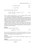
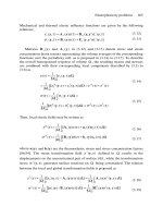
Return to Eqs. (7.13) and (7.20) based on the assumption that the coefficients of thermal
expansion do not depend on temperature. For moderate temperatures, this is a reasonable
approximation. This conclusion follows from Fig. 7.6, in which the experimental results
of Sukhanov et al. (1990) (shown with solid lines) are compared with Eqs. (7.20), in which
T = T − 20
◦
C (dashed lines) represent carbon–epoxy angle-ply laminates. However,
for relatively high temperatures, some deviation from linear behavior can be observed.
In this case, Eqs. (7.13) and (7.20) for thermal strains can be generalized as
ε
T
=

T
T
0
α(T )dT
Chapter 7. Environmental, special loading, and manufacturing effects 375
−30
−20
−10
10
20
30

−100 −50 50
100
±10°
±10°
0°
0°
90°
90°
±45°
±45°
T,°C
10
5
ε
T
x
Fig. 7.6. Experimental dependencies of thermal strains on temperature (solid lines) for ±φ angle-ply carbon–
epoxy composite and the corresponding linear approximations (dashed lines).
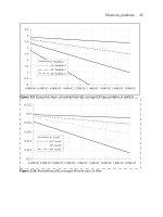
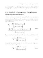
Temperature variations can also result in a change in material mechanical properties.
As follows from Fig. 7.7, in which the circles correspond to the experimental data of
Ha and Springer (1987), elevated temperatures result in either higher or lower reduction
of material strength and stiffness characteristics, depending on whether the corresponding
material characteristic is controlled mainly by the fibers or by the matrix. The curves
presented in Fig. 7.7 correspond to a carbon–epoxy composite, but they are typical
for polymeric unidirectional composites. The longitudinal modulus and tensile strength,
being controlled by the fibers, are less sensitive to temperature than longitudinal com-
pressive strength, and transverse and shear characteristics. Analogous results for a more
temperature-sensitive thermoplastic composite studied by Soutis and Turkmen (1993) are
presented in Fig. 7.8. Metal matrix composites demonstrate much higher thermal resis-
tance, whereas ceramic and carbon–carbon composites have been specially developed to

withstand high temperatures. For example, carbon–carbon fabric composite under heat-
ing up to 2500
◦
C demonstrates only a 7% reduction in tensile strength and about 30%
reduction in compressive strength without significant change of stiffness.
Analysis of thermoelastic deformation for materials whose stiffness characteristics
depend on temperature presents substantial difficulties because thermal strains are caused
not only by material thermal expansion, but also by external forces. Consider, for example,
a structural element under temperature T
0
loaded with some external force P
0
, and assume
that the temperature is increased to a value T
1
. Then, the temperature change will cause a
thermal strain associated with material expansion, and the force P
0
, being constant, also
induces additional strain because the material stiffness at temperature T
1
is less than its
stiffness at temperature T
0
. To determine the final stress and strain state of the structure,
376 Advanced mechanics of composite materials
+
s
1
−

+
E
2
E
1
G
12
0
0.2
0.4
0.6
0.8
1
0 50 100 150 200
T,°C
t
12
s
2
s
1
Fig. 7.7. Experimental dependencies of normalized stiffness (solid lines) and strength (dashed lines) character-
istics of unidirectional carbon–epoxy composite on temperature.
0
0.2
0.4
0.6
0.8
1
0 40 80 120

T,°C
E
1
E
2
s
−
1
s
+
2
s
+
1
Fig. 7.8. Experimental dependencies of normalized stiffness (solid lines) and strength (dashed lines) character-
istics of unidirectional glass–polypropylene composite on temperature.
Chapter 7. Environmental, special loading, and manufacturing effects 377
we should describe the process of loading and heating using, e.g., the method of successive
loading (and heating) presented in Section 4.1.2.
7.2. Hygrothermal effects and aging
Effects that are similar to temperature variations, i.e., expansion and degradation of
properties, can also be caused by moisture. Moisture absorption is governed by Fick’s
law, which is analogous to Fourier’s law, Eq. (7.1), for thermal conductivity, i.e.,
q
W
=−D
∂
W
∂
n

(7.31)
in which q
W
is the diffusion flow through a unit area of surface with normal n, D is the
diffusivity of the material whose moisture absorption is being considered, and W is the
relative mass moisture concentration in the material, i.e.,
W =
m
m
(7.32)
where m is the increase in the mass of a unit volume material element due to mois-
ture absorption and m is the mass of the dry material element. Moisture distribution
in the material is governed by the following equation, similar to Eq. (7.2) for thermal
conductivity
∂
∂
n

D
∂
W
∂
n

=
∂
W
∂
t
(7.33)

Consider a laminated composite material shown in Fig. 7.9 for which n coincides with the
z axis. Despite the formal correspondence between Eq. (7.2) for thermal conductivity and
Eq. (7.32) for moisture diffusion, there is a difference in principle between these problems.
This difference is associated with the diffusivity coefficient D, which is much lower than
z
W
m
W
m
W
m
h
h
x
x
z
(b)(a)
Fig. 7.9. Composite material exposed to moisture on both surfaces z = 0 and z = h (a), and on the surface
z = 0 only (b).
378 Advanced mechanics of composite materials
the thermal conductivity λ of the same material. As is known, there are materials, e.g.,
metals, with relatively high λ and practically zero D coefficients. Low D-value means
that moisture diffusion is a rather slow process. As shown by Shen and Springer (1976),
the temperature increase in time inside a surface-heated composite material reaches a
steady (equilibrium) state temperature about 10
6
times faster than the moisture content
approaching the corresponding stable state. This means that, in contrast to Section 7.1.1 in
which the steady (time-independent) temperature distribution is studied, we must consider
the time-dependent process of moisture diffusion. To simplify the problem, we can neglect

the possible variation of the mass diffusion coefficient D over the laminate thickness,
taking D = constant for polymeric composites. Then, Eq. (7.33) reduces to
D
∂
2
W
∂
z
2
=
∂
W
∂
t
(7.34)
Consider the laminate in Fig. 7.9a. Introduce the maximum moisture content W
m
that
can exist in the material under the preassigned environmental conditions. Naturally, W
m
depends on the material nature and structure, temperature, relative humidity (RH)ofthe
gas (e.g., humid air), or on the nature of the liquid (distilled water, salted water, fuel,
lubricating oil, etc.) to the action of which the material is exposed. Introduce also the
normalized moisture concentration as
w(z, t) =
W(z,t)
W
m
(7.35)
Obviously, for t →∞, we have w → 1. Then, the function w(z, t) can be presented in

the form
w(z, t) = 1 −
∞

n=1
w
n
(z)e
−k
n
t
(7.36)
Substitution into Eq. (7.34), with due regard to Eq. (7.35), yields the following ordinary
differential equation
w

n
+r
2
n
w
n
= 0
in which r
2
n
= k
n
/D and ()


= d()/dz. The general solution is
w
n
= C
1n
sin r
n
z +C
2n
cos r
n
z
The integration constants can be found from the boundary conditions on the surfaces z = 0
and z = h (see Fig. 7.9a). Assume that on these surfaces W = W
m
or w = 1. Then, in
accordance with Eq. (7.36), we get
w
n
(0,t)= 0,w
n
(h, t) = 0 (7.37)
Chapter 7. Environmental, special loading, and manufacturing effects 379
The first of these conditions yields C
2n
= 0, whereas from the second condition we have
sin r
n
h = 0, which yields
r

n
h = (2n −1)π (n = 1, 2, 3, ) (7.38)
Thus, the solution in Eq. (7.36) takes the form
w(z, t) = 1 −
∞

n=1
C
1n
sin

2n −1
h
πz

exp

−

2n −1
h

2
π
2
Dt

(7.39)
To determine C
1n

, we must use the initial condition, according to which
w(0 <z<h,t= 0) = 0
Using the following Fourier series
1 =
4
π
∞

n=1
sin(2n −1)z
2n −1
we get C
1n
= 4/(2n −1)π, and the solution in Eq. (7.39) can be written in its final form
w(z, t) = 1 −
4
π
∞

n=1
sin(2n −1)πz
2n −1
exp

−

2n −1
h

2

π
2
Dt

(7.40)
where
z = z/ h.
For the structure in Fig. 7.9b, the surface z = h is not exposed to moisture, and hence
q
W
(z = h) = 0. So, in accordance with Eq. (7.31), the second boundary condition in
Eqs. (7.37) must be changed to w

(h, t) = 0. Then, instead of Eq. (7.38), we must use
r
n
h =
π
2
(2n −1)
Comparing this result with Eq. (7.38), we can conclude that for the laminate in Fig. 7.9b,
w(z, t) is specified by the solution in Eq. (7.40) in which we must change h to 2h.
The mass increase of the material with thickness h is
M = A

h
0
mdz
where A is the surface area. Using Eqs. (7.32) and (7.35), we get
M = AmW

m

h
0
wdz
380 Advanced mechanics of composite materials
Switching to a dimensionless variable z = z/ h and taking the total moisture content as
C =
M
Amh
(7.41)
we arrive at
C = W
m

1
0
w dz
where w is specified by Eq. (7.40). Substitution of this equation and integration yields
C =
C
W
m
= 1 −
8
π
2
∞

n=1

1
(2n −1)
2
exp

−

2n −1
h

2
π
2
Dt

(7.42)
For numerical analysis, consider a carbon–epoxy laminate for which D = 10
−3
mm
2
/
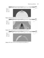
hour (Tsai, 1987) and h = 1 mm. The distributions of the moisture concentration over the
laminate thickness are shown in Fig. 7.10 for t = 1, 10, 50, 100, 200, and 500 h. As can be
seen, complete impregnation of 1-mm-thick material takes about 500 h. The dependence
of
Con t found in accordance with Eq. (7.42) is presented in Fig. 7.11.
An interesting interpretation of the curve in Fig. 7.11 can be noted if we change the vari-
able t to
√
t. The resulting dependence is shown in Fig. 7.12. As can be seen, the initial

0
0.2
0.4
0.6
0.8
1
0 0.2 0.4 0.6 0.8 1
w(z,t)
z
t = 500 hours
200
100
50
10
1
Fig. 7.10. Distribution of the normalized moisture concentration w over the thickness of 1-mm-thick carbon–
epoxy composite for various exposure times t.
Chapter 7. Environmental, special loading, and manufacturing effects 381
C(t)
t, hours
0
0.2
0.4
0.6
0.8
1
0 100 200 300 400 500
Fig. 7.11. Dependence of the normalized moisture concentration C on time t.
0
0.2

0.4
0.6
0.8
1
0 5 10 15 20 25
t)C(
hourt,
Fig. 7.12. Dependence of the normalized moisture concentration on
√
t.
part of the curve is close to a straight line whose slope can be used to determine the
diffusion coefficient of the material matching the theoretical dependence C(t) with the
experimental one. Note that experimental methods usually result in rather approximate
evaluation of the material diffusivity D with possible variations up to 100% (Tsai, 1987).
The maximum value of the function C(t) to which it tends to approach determines the
maximum moisture content C
m
= W
m
.
382 Advanced mechanics of composite materials
0
0.4
0.8
1.2
1.6
01020 304050
C(t),%
hourt ,
3

2
1
Fig. 7.13. Dependence of the moisture content on time for a carbon–epoxy composite exposed to air with
45% RH (1), 75% RH (2), 95% RH (3).
Thus, the material behavior under the action of moisture is specified by two experimen-
tal parameters – D and C
m
– which can depend on the ambient media, its moisture content,
and temperature. The experimental dependencies of C in Eq. (7.41) on t for 0.6-mm-thick
carbon–epoxy composite exposed to humid air with various relative humidity (RH ) levels
are shown in Fig. 7.13 (Survey, 1984). As can be seen, the moisture content is approxi-
mately proportional to the air humidity. The gradients of the curves in Fig. 7.13 depend
on the laminate thickness (Fig. 7.14, Survey, 1984).
0
0.4
0.8
1.2
1.6
01020304050
C(t),%
hourt,
3
2
1
Fig. 7.14. Dependencies of the moisture content on time for a carbon–epoxy composite with thickness
3.6 mm (1), 1.2 mm (2), and 0.6 mm (3) exposed to humid air with 75% RH.
Chapter 7. Environmental, special loading, and manufacturing effects 383
Among polymeric composites, the highest capacity for moisture absorption under room
temperature is demonstrated by aramid composites (7 ±0.25% by weight) in which both
the polymeric matrix and fibers are susceptible to moisture. Glass and carbon polymeric

composites are characterized with moisture content 3.5±0.2% and 2±0.75%, respectively.
In real aramid–epoxy and carbon–epoxy composite structures, the moisture content is
usually about 2% and 1%, respectively. The lowest susceptibility to moisture is demon-
strated by boron composites. Metal matrix, ceramic, and carbon–carbon composites are
not affected by moisture.
The material diffusivity coefficient D depends on temperature in accordance with the
Arrhenius relationship (Tsai, 1987)
D(T
a
) =
D
0
e
k/T
a
in which D
0
and k are some material constants and T
a
is the absolute temperature. Exper-
imental dependencies of the moisture content on time in a 1.2-mm-thick carbon–epoxy
composite exposed to humid air with 95% RH at various temperatures are presented
in Fig. 7.15 (Survey, 1984). The most pronounced effect of temperature is observed
for aramid–epoxy composites. The corresponding experimental results of Milyutin et al.
(1989) are shown in Fig. 7.16.
When a material absorbs moisture, it expands, demonstrating effects that are similar to
thermal effects, which can be modeled using the equations presented in Section 7.1.2, if
we treat α
1
,α

2
and α
x
,α
y
as coefficients of moisture expansion and change T for C.
Similar to temperature, increase in moisture reduces material strength and stiffness. For
carbon–epoxy composites, this reduction is about 12%, for aramid–epoxy composites,
about 25%, and for glass–epoxy materials, about 35%. After drying out, the effect of
moisture usually disappears.
0
0.4
0.8
1.2
010 2030 4050
C(t),%
hourt ,
1
2
3
Fig. 7.15. Dependencies of the moisture content on time for 1.2-mm-thick carbon–epoxy composite exposed to
humid air with 95% RH under temperatures 25
◦
C (1), 50
◦
C (2), and 80
◦
C (3).
384 Advanced mechanics of composite materials
0

4
8
12
16
01020304050
75°C
60°C
40°C
T=20°C
hour
t,
C(t),%
Fig. 7.16. Moisture content as a function of time and temperature for aramid–epoxy composites.
The cyclic action of temperature, moisture, or sun radiation results in material aging, i.e.,
in degradation of the material properties during the process of material or structure storage.
For some polymeric composites, exposure to elevated temperature, which can reach 70
◦
C,
and radiation, whose intensity can be as high as 1 kW/m
2
, can cause more complete curing
of the resin and some increase of material strength in compression, shear, or bending.
However, under long-term action of the aforementioned factors, the material strength
and stiffness decrease. To evaluate the effect of aging, testing under transverse bending
(see Fig. 4.98) is usually performed. The flexural strength obtained
σ
f
=
3
Pl

2bh
2
allows for both fiber and matrix material degradation in the process of aging. Experimental
results from G.M. Gunyaev et al. showing the dependence of the normalized flexural
strength on time for advanced composites are presented in Fig. 7.17. The most dramatic
is the effect of aging on the ultimate transverse tensile deformation
ε
2
of unidirectional
composites: the low value of which results in cracking of the matrix as discussed in
Sections 4.4.2 and 6.4. After accelerated aging, i.e., long-term moisture conditioning at
temperature 70
◦
C, a 0.75% moisture content in carbon–epoxy composites results in about
20% reduction of
ε
2
, whereas a 1.15% moisture content causes about 45% reduction.
Environmental effects on composite materials are discussed in detail elsewhere
(Tsai, 1987; Springer, 1981, 1984, 1988).
Chapter 7. Environmental, special loading, and manufacturing effects 385
0
0.2
0.4
0.6
0.8
1
012 345
t, yea
r

1
2
4
3
s
f
Fig. 7.17. Dependence of the normalized flexural strength on the time of aging for boron (1), carbon (2),
aramid (3), and glass (4) epoxy composites.
7.3. Time and time-dependent loading effects
7.3.1. Viscoelastisity
Polymeric matrices are characterized with pronounced viscoelastic properties result-
ing in time-dependent behavior of polymeric composites that manifests itself in creep
(see Section 1.1), stress relaxation, and dependence of the stress–strain diagram on the
rate of loading. It should be emphasized that in composite materials, viscoelastic defor-
mation of the polymeric matrix is restricted by the fibers that are usually linear elastic
and do not demonstrate time-dependent behavior. The one exception to existing fibers
is represented by aramid fibers that are actually polymeric themselves by their nature.
The properties of metal matrix, ceramic, and carbon–carbon composites under normal
conditions do not depend on time. Rheological (time-dependent) characteristics of struc-
tural materials are revealed in creep tests allowing us to plot the dependence of strain on
time under constant stress. Such diagrams are shown in Fig. 7.18 for the aramid–epoxy
composite described by Skudra et al. (1989). An important characteristic of the mate-
rial can be established if we plot the so-called isochrone stress–strain diagrams shown in
Fig. 7.19. Three curves in this figure are plotted for t = 0, t = 100, and t = 1000 days,
and the points on these curves correspond to points 1, 2, 3 in Fig. 7.18. As can be seen,
the initial parts of the isochrone diagrams are linear, which means that under moderate
stress, the material under study can be classified as a linear-viscoelastic material. To char-
acterize such a material, we need to have only one creep diagram, whereby the other
curves can be plotted, increasing strains in proportion to stress. For example, the creep
curve corresponding to σ

1
= 450 MPa in Fig. 7.18 can be obtained if we multiply strains
corresponding to σ
1
= 300 MPa by 1.5.
386 Advanced mechanics of composite materials
3
0
0.5
1
1.5
0 200 400 600 800 1000
3
2
1
2
1
t, Days (24 hours)
s
1
= 600 MPa
s
1
= 450 MPa
s
1
= 300 MPa
e
1
,%

e
1
0
Fig. 7.18. Creep strain response of unidirectional aramid–epoxy composite under tension in longitudinal
direction with three constant stresses.
0
200
400
600
0 0.5 1 1.5
s
1
, MPa
t = 0
t = 100
t = 1000
1
1
2
2
3
3
e
1
,%
Fig. 7.19. Isochrone stress–strain diagrams corresponding to creep curves in Fig. 7.18.
Linear-viscoelastic material behavior is described with reasonable accuracy by the
hereditary theory, according to which the dependence of strain on time is expressed as
ε(t) =
1

E

σ(t)+

t
0
C(t −τ)σ(τ)dτ

(7.43)
Here, t is the current time, τ is some moment of time in the past (0 ≤ τ ≤ t) at which
stress σ(τ) acts, and C(t − τ) is the creep compliance (or creep kernel) depending on
time passing from the moment τ to the moment t. The constitutive equation of hereditary
theory, Eq. (7.43), is illustrated in Fig. 7.20. As can be seen, the total strain ε(t) is
composed of the elastic strain ε
e
governed by the current stress σ(t) and the viscous
Chapter 7. Environmental, special loading, and manufacturing effects 387
s
t
t
dt
t
tt − t
E
e
s(t)
s(t)
e
e
=

s (t)
e
v
t
t
Fig. 7.20. Geometric interpretation of the hereditary constitutive theory.
strain ε
v
depending on the loading process as if the material ‘remembers’ this process.
Within the framework of this interpretation, the creep compliance C(θ), where θ = t −τ
can be treated as some ‘memory function’ that should, obviously, be infinitely high at
θ = 0 and tend to zero for θ →∞, as in Fig. 7.21.
The inverse form of Eq. (7.43) is
σ(t) = E

ε(t) −

t
0
R(t −τ)ε(τ)dτ

(7.44)
Here, R(t − τ) is the relaxation modulus or the relaxation kernel that can be expressed,
as shown below, in terms of C(t − τ).
The creep compliance is determined using experimental creep diagrams. Transforming
to a new variable θ = t −τ, we can write Eq. (7.43) in the following form
ε(t) =
1
E


σ(t)+

t
0
C(θ)σ(θ −t)dθ

(7.45)
388 Advanced mechanics of composite materials
q = t –
t
C(q)
Fig. 7.21. Typical form of the creep compliance function.
For a creep test, the stress is constant, so σ = σ
0
, and Eq. (7.44) yields
ε(t) = ε
0

1 +

t
0
C(θ)dθ

(7.46)
where ε
0
= σ
0
/E = ε(t = 0) is the instantaneous elastic strain (see Fig. 7.18). Differen-

tiating this equation with respect to t,weget
C(t) =
1
ε
0
dε(t)
dt
x
This expression allows us to determine the creep compliance by differentiating the given
experimental creep diagram or its analytical approximation. However, for practical analy-
sis, C(θ) is usually determined directly from Eq. (7.46) introducing some approximation
for C(θ) and matching the function obtained ε(t) with the experimental creep diagram.
For this purpose, Eq. (7.46) is written in the form
ε(t)
ε
0
= 1 +

t
0
C(θ)dθ (7.47)
Experimental creep diagrams for unidirectional glass–epoxy composite are presented in
this form in Fig. 7.22 (solid lines).
The simplest form is an exponential approximation of the type
C(θ) =
N

n=1
A
n

e
−α
n
θ
(7.48)
Chapter 7. Environmental, special loading, and manufacturing effects 389
1
1.2
1.4
1.6
1.8
2
0 50 100 150
,,
(24 hours)t, Days
e
1
e
1
0
e
2
0
g
12
e
2
g
12
e

1
/e
1
0
e
2
/e
2
0
g
12
/g
0
12
0
Fig. 7.22. Creep strain diagrams for unidirectional glass–epoxy composite (solid lines) under tension in longi-
tudinal direction (ε
1
/ε
0
1
), transverse direction (ε
2
/ε
0
2
), and under in-plane shear (γ
12
/γ
0

12
) and the corresponding
exponential approximations (dashed lines).
Substituting Eq. (7.48) into Eq. (7.47), we obtain
ε(t)
ε
0
= 1 +
N

n=1
A
n
α
n
(1 −e
−α
n
t
)
For the curves presented in Fig. 7.22, calculation yields
• longitudinal tension: N = 1, A
1
= 0;
• transverse tension: N = 1, A
1
= 0.04, α
1
= 0.06 1/day;
• in-plane shear: N = 2, A

1
= 0.033, α
1
= 0.04 1/day, A
2
= 0.06, α
2
= 0.4 1/day.
The corresponding approximations are shown in Fig. 7.22 with dashed lines. The main
shortcoming of the exponential approximation in Eq. (7.48) is associated with the fact
that, in contrast to Fig. 7.21, C(θ) has no singularity at θ = 0, which means that it cannot
properly describe material behavior in the vicinity of t = 0.
It should be emphasized that the one-term exponential approximation corresponds to
a simple rheological mechanical model shown in Fig. 7.23. The model consists of two
linear springs simulating material elastic behavior in accordance with Hooke’s law
σ
1
= E
1
ε
1
,σ
2
= E
2
ε
2
(7.49)
and one dash-pot simulating material viscous behavior obeying the Newton flow law
σ

v
= η
dε
v
dt
(7.50)
390 Advanced mechanics of composite materials
s, e
E
1
, s
1
, e
1
s, e
E
2
, s
2
, e
2
h, s
v
, e
v
Fig. 7.23. Three-element mechanical model.
Equilibrium and compatibility conditions for the model in Fig. 7.23 are
σ = σ
2
+σ

v
,σ
1
= σ
ε
v
= ε
2
,ε
1
+ε
2
= ε
Using the first of these equations and Eqs. (7.49)–(7.50), we get
σ = E
2
ε
2
+η
dε
v
dt
Taking into account that
ε
2
= ε
v
= ε −
σ
E

we finally arrive at the following constitutive equation relating the apparent stress σ to
the apparent strain ε
σ

1 +
E
2
E
1

+
η
E
1
dσ
dt
= E
2
ε + η
dε
dt
(7.51)
This equation allows us to introduce some useful material characteristics. Indeed, consider
a very fast loading, i.e., such that stress σ and strain ε can be neglected in comparison
Chapter 7. Environmental, special loading, and manufacturing effects 391
with their rates. Then, integration yields σ = E
i
ε, where E
i
= E

1
is the instantaneous
modulus of the material. Now assume that the loading is so slow that stress and strain
rates can be neglected. Then, Eq. (7.51) yields σ = E
l
ε, where
E
l
=
E
1
E
2
E
1
+E
2
(7.52)
is the long-time modulus.
We can now apply the model under study to describe material creep. Taking σ = σ
0
and integrating Eq. (7.51) with initial condition ε
0
(0) = σ
0
/E, we get
ε =
σ
0
E

1

1 +
E
1
E
2

1 −e
E
2
η
t

The corresponding creep diagram is shown in Fig. 7.24. As follows from this figure,
ε(t →∞) = σ
0
/E
l
, where E
l
is specified by Eq. (7.52). This means that there exists
some limit for the creep strain, and materials that can be described with this model should
possess the so-called limited creep.
Now assume that the model is loaded in such a way that the apparent strain is
constant, i.e., that ε = ε
0
. Then, the solution of Eq. (7.51) that satisfies the condition
σ(0) = E
1

ε
0
is
σ =
E
1
ε
0
E
1
+E
2

E
2
+E
1
e
−t/t
r

,t
r
=
η
E
1
+E
2
The corresponding dependence is presented in Fig. 7.25 and illustrates the process of

stress relaxation. The parameter t
r
is called the time of relaxation. During this time, the
stress decreases by the factor of e.
Consider again Eq. (7.51) and express E
1
,E
2
, and η in terms of E
i
,E
l
, and t
r
. The
resulting equation is as follows
σ + t
r
dσ
dt
= E
l
ε + E
i
t
r
dε
dt
(7.53)
E

i
t
E
l
s
0
s
0
e
Fig. 7.24. Creep diagram corresponding to the mechanical model in Fig. 7.23.
392 Advanced mechanics of composite materials
E
i
e
0
t
r
e
s
E
l
e
0
t
s
Fig. 7.25. Relaxation diagram corresponding to the mechanical model in Fig. 7.23.
This first-order differential equation can be solved for ε in the general case. Omitting
rather cumbersome transformations, we arrive at the following solution
ε(t) =
1

E
i

σ(t)+
1
t
r

1 −
E
l
E
i


t
0
e
−
E
l
E
i
t
r
(t−τ)
σ(τ)dτ

This result corresponds to Eq. (7.45) of the hereditary theory with one-term exponential
approximation of the creep compliance in Eq. (7.48), in which N = 1. Taking more terms

in Eq. (7.48), we get more flexibility in the approximation of experimental results with
exponential functions. However, the main features of material behavior are, in principle,
the same as that for the one-term approximation (see Figs. 7.23 and 7.24). In particular,
there exists the long-time modulus that follows from Eq. (7.46) if we examine the limit
for t →∞, i.e.,
ε(t) →
σ
0
E
l
,E
l
=
E
1 +

∞
0
C(θ)dθ
For the exponential approximation in Eq. (7.48),
I =

∞
0
C(θ)dθ =
N

n=1
A
n

α
n
Since the integral I has a finite value, the exponential approximation of the creep com-
pliance can be used only for materials with limited creep. There exist more complicated
singular approximations, e.g.,
C(θ) =
A
θ
α
, C(θ) =
A
θ
α
e
−βθ
Chapter 7. Environmental, special loading, and manufacturing effects 393
for which I →∞and E
l
= 0. This means that for such materials, the creep strain can
be infinitely high.
A useful interpretation of the hereditary theory constitutive equations can be constructed
with the aid of the integral Laplace transformation, according to which a function f(t)is
associated with its Laplace transform f
∗
(p) as
f
∗
(p) =

∞

0
f(t)e
−pt
dt
For some functions that we need to use for the examples presented below, we have
f(t)= 1,f
∗
(p) =
1
p
f(t)= e
−αt
,f
∗
(p) =
1
α + p
(7.54)
The importance of the Laplace transformation for the hereditary theory is associated with
the existence of the so-called convolution theorem, according to which


t
0
f
1
(θ)f
2
(θ −t)dθ


∗
= f
∗
1
(p)f
∗
2
(p)
Using this theorem and applying Laplace transformation to Eq. (7.45), we get
ε
∗
(p) =
1
E

σ
∗
(p) +C
∗
(p)σ
∗
(p)

This result can be presented in a form similar to Hookes’s law, i.e.,
σ
∗
(p) = E
∗
(p)ε
∗

(p) (7.55)
where
E
∗
=
E
1 +C
∗
(p)
Applying Laplace transformation to Eq. (7.44), we arrive at Eq. (7.55) in which
E
∗
= E[1 −R
∗
(p)] (7.56)
Comparing Eqs. (7.55) and (7.56), we can relate Laplace transforms of the creep
compliance to the relaxation modulus, i.e.,
1
1 +C
∗
(p)
= 1 − R
∗
(p)
With due regard to Eq. (7.55), we can formulate the elastic–viscoelastic analogy or
the correspondence principle, according to which the solution of the linear viscoelasticity
394 Advanced mechanics of composite materials
problem can be obtained in terms of the corresponding Laplace transforms from the
solution of the linear elasticity problem if E is replaced with E
∗

and all the stresses,
strains, displacements, and external loads are replaced with their Laplace transforms.
For an orthotropic material in a plane stress state, e.g., for a unidirectional composite ply
or layer referred to the principal material axes, Eqs. (4.55) and (7.43) can be generalized as
ε
1
(t) =
1
E
1

σ
1
(t) +

t
0
C
11
(t −τ)σ
1
(τ )dτ

−
ν
12
E
2

σ

2
(t) +

t
0
C
12
(t −τ)σ
2
(τ )dτ

ε
2
(t) =
1
E
2

σ
2
(t) +

t
0
C
22
(t −τ)σ
2
(τ )dτ


−
ν
21
E
1

σ
1
(t) +

t
0
C
21
(t −τ)σ
1
(τ )dτ

γ
12
(t) =
1
G
12

τ
12
(t) +

t

0
K
12
(t −τ)τ
12
(τ )dτ

Applying Laplace transformation to these equations, we can reduce them to a form similar
to Hooke’s law, Eqs. (4.55), i.e.,
ε
∗
1
(p) =
σ
∗
1
(p)
E
∗
1
(p)
−
ν
∗
12
(p)
E
∗
2
(p)

σ
∗
2
(p)
ε
∗
2
(p) =
σ
∗
2
(p)
E
∗
2
(p)
−
ν
∗
21
(p)
E
∗
1
(p)
σ
∗
1
(p)
γ

∗
12
(p) =
τ
∗
12
(p)
G
∗
12
(p)
(7.57)
where
E
∗
1
(p) =
E
1
1 +C
∗
11
(p)
,E
∗
2
(p) =
E
2
1 +C

∗
22
(p)
,G
∗
12
(p) =
G
12
1 +K
∗
12
(p)
ν
∗
12
(p) =
1 +C
∗
12
(p)
1 +C
∗
22
(p)
ν
12
,ν
∗
21

(p) =
1 +C
∗
21
(p)
1 +C
∗
11
(p)
ν
21
(7.58)
For the unidirectional composite ply whose typical creep diagrams are shown in Fig. 7.22,
the foregoing equations can be simplified by neglecting material creep in the longitudinal
direction (C
11
= 0) and assuming that Poisson’s effect is linear elastic and symmetric,
Chapter 7. Environmental, special loading, and manufacturing effects 395
i.e., that
ν
∗
12
E
∗
2
=
ν
12
E
2

,
ν
∗
21
E
∗
1
=
ν
21
E
1
Then, Eqs. (7.57) take the form
ε
∗
1
(p) =
σ
∗
1
(p)
E
1
−
ν
12
E
2
σ
∗

2
(p)
ε
∗
2
(p) =
σ
∗
2
(p)
E
∗
2
−
ν
21
E
1
σ
∗
1
(p)
γ
∗
12
(p) =
τ
∗
12
(p)

G
∗
12
(p)
(7.59)
Supplementing constitutive equations, Eqs. (7.57) or (7.59), with strain-displacement and
equilibrium equations written in terms of Laplace transforms of stresses, strains, displace-
ments, and external loads and solving the problem of elasticity, we can find Laplace
transforms for all the variables. To represent the solution obtained in this way in terms of
time t, we need to take the inverse Laplace transformation, and this is the most difficult
stage of the problem solution. There exist exact and approximate analytical and numerical
methods for performing the inverse Laplace transformation discussed, for example, by
Schapery (1974). The most commonly used approach is based on approximation of the
solution written in terms of the transformation parameter p with some functions for which
the inverse Laplace transformation is known.
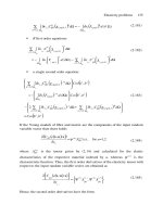
As an example, consider the problem of torsion for an orthotropic cylindrical shell
similar to that shown in Fig. 6.20. The shear strain induced by torque T is specified
by Eq. (5.163). Using the elastic–viscoelastic analogy, we can write the corresponding
equation for the creep problem as
γ
∗
xy
(p) =
T
∗
(p)
2πR
2
B
∗

44
(p)
(7.60)
Here, B
∗
44
(p) = A
∗
44
(p)h, where h is the shell thickness.
Let the shell be made of glass–epoxy composite whose mechanical properties are listed
in Table 3.5 and creep diagrams are shown in Fig. 7.22. To simplify the analysis, we
suppose that for the unidirectional composite under study E
2
/E
1
= 0.22, G
12
/E
1
= 0.06,
and ν
12
= ν
21
= 0, and introduce the normalized shear strain
γ = γ
xy

T

R
2
hE
1

−1
396 Advanced mechanics of composite materials
Consider a ±45
◦
angle-ply material discussed in Section 4.5 for which, with due regard
to Eqs. (4.72), and (7.58), we can write
A
∗
44
(p) =
1
4

E
1
+E
∗
2

=
1
4

E
1

+
E
2
1 +C
∗
22
(p)

Exponential approximation, Eq. (7.48), of the corresponding creep curve in Fig. 7.22 (the
lower dashed line) is
C
22
= A
1
e
−α
1
θ
where A
1
= 0.04 and α
1
= 0.06 1/day. Using Eqs. (7.54), we arrive at the following
Laplace transforms of the creep compliance and the torque which is constant
C
∗
22
(p) =
A
1

α
1
+p
,T
∗
(p) =
T
p
The final expression for the Laplace transform of the normalized shear strain is
γ
∗
(p) =
2E(α
1
+A
1
+p)
πp(α
1
+A
1
E +p)
(7.61)
where E = E
1
/(E
1
+E
2
)

To use Eqs. (7.54) for the inverse Laplace transformation, we should decompose the
right-hand part of Eq. (7.61) as
γ
∗
(p) =
2E
π(α
1
+A
1
E)

α
1
+A
1
p
−
A
1
(1 −E)
α
1
+A
1
E +p

Applying Eqs. (7.54), we get
γ(t) =
2E

π(α
1
+A
1
E)

α
1
+A
1
−A
1
(1 −E)e
−(α
1
+A
1
E)t

This result is demonstrated in Fig. 7.26. As can be seen, there is practically no creep
because the cylinder’s deformation is controlled mainly by the fibers.
Quite different behavior is demonstrated by the cylinder made of 0
◦
/90
◦
cross-ply
composite material discussed in Section 4.4. In accordance with Eqs. (4.114) and (7.58),
we have
A
∗

44
(p) = G
∗
12
(p) =
G
12
1 +K
∗
12
(p)
Exponential approximation, Eq. (7.48), of the shear curve in Fig. 7.22 (the upper dashed
line) results in the following equation for the creep compliance
K
12
= A
1
e
−α
1
θ
+A
2
e
−α
2
θ