Chapter 6. Failure criteria and strength of laminates 337
For tension in the directions of axes 1

and 2

in Fig. 6.16 and for shear in plane 1

2

,we
can write Eq. (6.25) in the following forms similar to Eqs. (6.10)
F

σ
45
1
= σ
45
,σ
45
2
= 0,τ
45
12
= 0

= 1
F

σ
45

1
= 0,σ
45
2
= σ
45
,τ
45
12
= 0

= 1
F

σ
45
1
= 0,σ
45
2
= 0,τ
45
12
= τ
45

= 1
(6.26)
Here,
σ

45
and τ
45
determine material strength in coordinates 1

and 2

(see Fig. 6.16).
Then, Eq. (6.25) can be reduced to
F

σ
45
1
,σ
45
2
,τ
45
12

=
1
σ
2
45


σ
45

1

2
+

σ
45
2

2

+

1
τ
2
45
−
2
σ
2
45

σ
45
1
σ
45
2
+


τ
45
12
τ
45

=1
(6.27)
where
σ
45
and τ
45
are given by
1
σ
2
45
=
1
4

2
σ
2
0
+
1
τ

2
0

,
τ
2
45
=
1
2
σ
2
0
Comparing Eq. (6.27) with Eq. (6.23), we can see that Eq. (6.27), in contrast to Eq. (6.23),
includes a term with the product of stresses σ
45
1
and σ
45
2
. So, the strength criterion under
study changes its form with a transformation of the coordinate frame (from 1 and 2 to 1

and 2

in Fig. 6.16) which means that the approximation polynomial strength criterion in
Eq. (6.23) and, hence, the original criterion in Eq. (6.21) is not invariant with respect to
the rotation of the coordinate frame.
Consider the class of invariant strength criteria which are formulated in a tensor-
polynomial form as linear combinations of mixed invariants of the stress tensor σ

ij
and
the strength tensors of different ranks S
ij
,S
ij kl
, etc., i.e.,

i, k
S
ik
σ
ik
+

i, k, m, n
S
ikmn
σ
ik
σ
mn
+···=1 (6.28)
Using the standard transformation for tensor components we can readily write this equation
for an arbitrary coordinate frame. However, the fact that the strength components form
a tensor induces some conditions that should be imposed on these components and not
necessarily correlate with experimental data.
To be specific, consider a second-order tensor criterion. Introducing contracted nota-
tions for tensor components and restricting ourselves to the consideration of orthotropic
338 Advanced mechanics of composite materials

materials referred to the principal material coordinates 1 and 2 (see Fig. 6.16), we can
present Eq. (6.22) as
F
(
σ
1
,σ
2
,τ
12
)
= R
0
1
σ
1
+R
0
2
σ
2
+R
0
11
σ
2
1
+2R
0
12

σ
1
σ
2
+R
0
22
σ
2
2
+4S
0
12
τ
2
12
= 1
(6.29)
which corresponds to Eq. (6.28) if we put
σ
11
= σ
1
,σ
12
= τ
12
,σ
22
= σ

2
and S
11
= R
1
,S
22
= R
2
,S
1111
= R
0
11
,
S
1122
= S
2211
= R
0
12
,S
2222
= R
0
22
,S
1212
= S

2121
= S
1221
= S
2112
= S
0
12
The superscript ‘0’ indicates that the components of the strength tensors are referred to
the principal material coordinates. Applying the strength conditions in Eqs. (6.14), we can
reduce Eq. (6.29) to the following form
F(σ
1
,σ
2
,τ
12
) = σ
1

1
σ
+
1
−
1
σ
−
1


+σ
2

1
σ
+
2
−
1
σ
−
2

+
σ
2
1
σ
+
1
σ
−
1
+2R
0
12
σ
1
σ
2

+
σ
2
2
σ
+
2
σ
−
2
+

τ
12
τ
12

2
= 1 (6.30)
This equation looks similar to Eq. (6.20), but there is a principal difference between them.
Whereas Eq. (6.20) is only an approximation to the experimental results, and we can take
any suitable value of coefficient R
12
(in particular, we put R
12
= 0), the criterion in
Eq. (6.30) has an invariant tensor form, and coefficient R
0
12
should be determined using

this property of the criterion.
Following Gol’denblat and Kopnov (1968) consider two cases of pure shear in coordi-
nates 1

and 2

shown in Fig. 6.17 and assume that τ
+
45
= τ
+
45
and τ
−
45
= τ
−
45
, where the
overbar denotes, as earlier, the ultimate value of the corresponding stress. In the general
case,
τ
+
45
= τ
−
45
. Indeed, for a unidirectional composite, stress τ
+
45

induces tension in
1′
1
2′
2
t
−
45
t
+
45
1′
1
2′
2
45° 45°
(a) (b)
Fig. 6.17. Pure shear in coordinates (1

, 2

) rotated by 45
◦
with respect to the principal material
coordinates (1, 2).

340 Advanced mechanics of composite materials
Substituting Eq. (6.34) into Eq. (6.33), we arrive at the final form of the criterion under
consideration
F

(
σ
1
,σ
2
,τ
12
)
=

σ
2
1
+σ
2
2

σ
2
0
+

2
σ
2
0
−
1
τ
2

45

σ
1
σ
2
+

τ
12
τ
0

2
= 1 (6.35)
Now, presenting Eq. (6.32) in the following matrix form
{
σ
}
T

R
0

{
σ
}
= 1 (6.36)
where
{

σ
}
=
⎧
⎪
⎨
⎪
⎩
σ
1
σ
2
τ
12
⎫
⎪
⎬
⎪
⎭
,

R
0

=
⎡
⎢
⎣
R
0

11
R
0
12
0
R
0
12
R
0
11
0
004S
0
12
⎤
⎥
⎦
R
0
11
=
1
σ
2
0
,R
0
12
=

1
σ
2
0
−
1
2τ
2
45
,S
0
12
=
1
4τ
2
0
(6.37)
Superscript ‘T’ means transposition converting the column vector
{
σ
}
into the row
vector
{
σ
}
T
.
Let us transform stresses referred to axes (1, 2) into stresses corresponding to axes

(1

and 2

) shown in Fig. 6.16. Such a transformation can be performed with the aid of
Eqs. (6.24). The matrix form of this transformation is
{
σ
}
=
[
T
]

σ
45

, (6.38)
where
[
T
]
=
⎡
⎢
⎢
⎢
⎢
⎢
⎣

1
2
1
2
−1
1
2
1
2
1
1
2
−
1
2
0
⎤
⎥
⎥
⎥
⎥
⎥
⎦
Substitution of the stresses in Eq. (6.38) into Eq. (6.36) yields

σ
45

T
[

T
]
T

R
0

[
T
]

σ
45

= 1
This equation, being rewritten as

σ
45

T

R
45

σ
45

= 1 (6.39)
Chapter 6. Failure criteria and strength of laminates 341

specifies the strength criterion for the same material but referred to coordinates (1

, 2

).
The strength matrix has the following form

R
45

=
[
T
]
T

R
0

[
T
]
=
⎡
⎢
⎣
R
45
11
R

45
12
0
R
45
12
R
45
11
0
004S
45
12
⎤
⎥
⎦
where
R
45
11
=
1
σ
2
0
+
1
4

1

τ
2
0
−
1
τ
2
45

R
45
12
=
1
σ
2
0
−
1
4

1
τ
2
0
+
1
τ
2
45


(6.40)
S
45
12
=
1
4τ
2
45
The explicit form of Eq. (6.39) is

1
σ
2
0
+
1
4

1
τ
2
0
−
1
τ
2
45




σ
45
1

2
+

σ
45
2

2

+2

1
σ
2
0
−
1
4

1
τ
2
0
+

1
τ
2
45

σ
45
1
σ
45
2
+

τ
45
12
τ
45

2
= 1 (6.41)
Now apply the strength conditions in Eqs. (6.26) to give
1
σ
2
45
=
1
σ
2

0
+
1
4

1
τ
2
0
−
1
τ
2
45

(6.42)
Then, the strength criterion in Eq. (6.41) can be presented as
F

σ
45
1
,σ
45
2
,τ
45
12

=

1
σ
2
45


σ
45
1

2
+

σ
45
2

2

+

2
σ
2
45
−
1
τ
2
0


σ
45
1
σ
45
2
+

τ
45
12
τ
45

2
= 1 (6.43)
Thus, we have two formulations of the strength criterion under consideration which are
specified by Eq. (6.35) for coordinates 1 and 2 and by Eq. (6.43) for coordinates 1

and 2

342 Advanced mechanics of composite materials
(see Fig. 6.16). As can be seen, Eqs. (6.35) and (6.43) have similar forms and follow from
each other if we change the stresses in accordance with the following rule
σ
1
↔ σ
45
1

,σ
2
↔ σ
45
2
,τ
12
↔ τ
45
12
, σ
0
↔ σ
45
, τ
0
↔ τ
45
However, such correlation is possible under the condition imposed by Eq. (6.42) which
can be presented in the form
I
s
=
1
σ
2
0
+
1
4τ

2
0
=
1
σ
2
45
+
1
4τ
2
45
(6.44)
This result means that I
s
is the invariant of the strength tensor, i.e., that its value does not
depend on the coordinate frame for which the strength characteristics entering Eq. (6.44)
have been found.
If the actual material characteristics do not satisfy Eq. (6.44), the tensor strength criterion
cannot be applied to this material. However, if this equation is consistent with experimental
data, the tensor criterion offers considerable possibilities to study material strength. Indeed,
restricting ourselves to two terms presented in Eq. (6.28) let us write this equation in
coordinates (1

, 2

) shown in Fig. 6.16 and suppose that φ = 45
◦
. Then


i, k
S
φ
ik
σ
φ
ik
+

i, k, m, n
S
φ
ikmn
σ
φ
ik
σ
φ
mn
= 1 (6.45)
Here, S
φ
ik
and S
φ
ikmn
are the components of the second and the fourth rank strength tensors
which are transformed in accordance with tensor calculus as
S
φ

ik
=

p, q
l
ip
l
kq
S
0
pq
S
φ
ikmn
=

p, q, r, s
l
ip
l
kq
l
mr
l
ns
S
0
pqrs
(6.46)
Here, l are directional cosines of axes 1


and 2

on the plane referred to coordinates 1 and 2
(see Fig. 6.16), i.e., l
11
= cos φ,l
12
= sin φ,l
21
=−sin φ, and l
22
= cos φ. Substitution
of Eqs. (6.46) in Eq. (6.45) yields the strength criterion in coordinates (1

, 2

) but written
in terms of strength components corresponding to coordinates (1, 2), i.e.,

i, k

p, q
l
ip
l
kq
S
0
pq

σ
φ
ik
+

i, k, m, n

p, q, r, s
l
ip
l
kq
l
mr
l
ns
S
0
pqrs
σ
φ
ik
σ
φ
mn
= 1 (6.47)
Chapter 6. Failure criteria and strength of laminates 343
Apply Eq. (6.47) to the special orthotropic material studied above (see Fig. 6.16) and for
which, in accordance with Eq. (6.22),
S

pq
= 0,S
1111
= S
2222
= R
0
11
= R
0
22
=
1
σ
2
0
S
1122
= S
2211
= R
0
12
=
1
σ
2
0
−
1

2τ
2
45
S
1212
= S
2121
= S
1221
= S
2112
= S
0
12
=
1
4τ
2
0
(6.48)
Following Gol’denblat and Kopnov (1968), consider the material strength under tension
in the 1

-direction and in shear in plane (1

, 2

). Taking first σ
φ
11

= σ
φ
,σ
φ
22
= 0,τ
φ
12
= 0
and then τ
φ
12
= τ
φ
,σ
φ
11
= 0,σ
φ
22
= 0, we get from Eq. (6.47)
σ
2
φ
=
1

p, q, r, s
l
1p

l
1q
l
1r
l
1s
S
0
pqrs
, τ
2
φ
=
1

p, q, r, s
l
1p
l
2q
l
1r
l
2s
S
0
pqrs
or in explicit form
σ
2

φ
=

R
0
11

cos
4
φ +sin
4
φ

+2

S
0
12
+2R
0
12

sin
2
φ cos
2
φ

−1
τ

2
φ
= 4

2

R
0
11
−R
0
12

sin
2
φ cos
2
φ +S
0
12
cos
2
2φ

−1
(6.49)
These equations allow us to calculate the material strength in any coordinate frame whose
axes make angle φ with the corresponding principal material axes. Taking into account
Eqs. (6.44) and (6.48), we can derive the following relationship from Eqs. (6.49)
1

σ
2
φ
+
1
4τ
2
φ
=
1
σ
2
0
+
1
4τ
2
0
= I
s
(6.50)
So, I
s
is indeed the invariant of the strength tensor whose value for a given material does
not depend on φ.
Thus, tensor-polynomial strength criteria provide universal equations that can be readily
written in any coordinate frame, but on the other hand, material mechanical characteristics,
particularly material strength in different directions, should follow the rules of tensor
transformation, i.e., composed invariants (such as I
s

) must be the same for all coordinate
frames.
6.1.4. Interlaminar strength
The failure of composite laminates can also be associated with interlaminar frac-
ture caused by transverse normal and shear stresses σ
3
and τ
13
,τ
23
or σ
z
and τ
xz
,τ
yz
344 Advanced mechanics of composite materials
(see Fig. 4.18). Since σ
3
= σ
z
and shear stresses in coordinates (1, 2, 3) are linked with
stresses in coordinates (x, y, z) by simple relationships in Eqs. (4.67) and (4.68), the
strength criterion is formulated here in terms of stresses σ
z
,τ
xz
,τ
yz
which can be found

directly from Eqs. (5.124). Since the laminate strength in tension and compression across
the layers is different, we can use the polynomial criterion similar to Eq. (6.15). For the
stress state under study, we get
σ
z

1
σ
+
3
−
1
σ
−
3

+

τ
r
τ
i

2
= 1 (6.51)
where
τ
r
=


τ
2
13
+τ
2
23
=

τ
2
xz
+τ
2
yz
is the resultant transverse shear stress, and τ
i
determines the interlaminar shear strength
of the material.
In thin-walled structures, the transverse normal stress is usually small and can be
neglected in comparison with the shear stress. Then, Eq. (6.51) can be simplified and
written as
τ
r
= τ
i
(6.52)
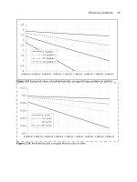
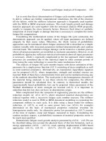
As an example, Fig. 6.18 displays the dependence of the normalized maximum deflection
w/R on the force P for a fiberglass–epoxy cross-ply cylindrical shell of radius R loaded
with a radial concentrated force P (Vasiliev, 1970). The shell failure was caused by
delamination. The shadowed interval shows the possible values of the ultimate force

0
0.4
0.8
1.2
1.6
2
0 0.004 0.008 0.012 0.016 0.02
P, kN
Rw
Fig. 6.18. Experimental dependence of the normalized maximum deflection of a fiberglass–epoxy cylindrical
shell on the radial concentrated force.
Chapter 6. Failure criteria and strength of laminates 345
calculated with the aid of Eq. (6.52) (this value is not unique because of the scatter in
interlaminar shear strength).
6.2. Practical recommendations
As follows from the foregoing analysis, for practical strength evaluation of fabric com-
posites, we can use either the maximum stress criterion, Eqs. (6.2) or second-order
polynomial criterion in Eq. (6.15) in conjunction with Eq. (6.16) for the case of biax-
ial compression. For unidirectional composites with polymeric matrices, we can apply
Eqs. (6.3) and (6.4) in which function F is specified by Eq. (6.18). It should be empha-
sized that experimental data usually have rather high scatter, and the accuracy of more
complicated and rigorous strength criteria can be more apparent than real.
Comparing tensor-polynomial and approximation strength criteria, we can conclude the
following. The tensor criteria should be used if our purpose is to develop a theory of mate-
rial strength, because a consistent physical theory must be covariant, i.e., the constraints
that are imposed on material properties within the framework of this theory should not
depend on a particular coordinate frame. For practical applications, the approximation cri-
teria are more suitable, but in the forms they are presented here they should be used only
for orthotropic unidirectional plies or fabric layers in coordinates whose axes coincide
with the fibers’ directions.

To evaluate the laminate strength, we should first determine the stresses acting in the
plies or layers (see Section 5.11), identify the layer that is expected to fail first and
apply one of the foregoing strength criteria. The fracture of the first ply or layer may not
necessarily result in failure of the whole laminate. Then, simulating the failed element with
a suitable model (see, e.g., Section 4.4.2), the strength analysis is repeated and continued
up to failure of the last ply or layer.
In principle, failure criteria can be constructed for the whole laminate as a quasi-
homogeneous material. This is not realistic for design problems, since it would be
necessary to compare the solutions for numerous laminate structures which cannot prac-
tically be tested. However, this approach can be used successfully for structures that are
well developed and in mass production. For example, the segments of two structures of
composite drive shafts – one made of fabric and the other of unidirectional composite,
are shown in Fig. 6.19. Testing these segments in tension, compression, and torsion, we
can plot the strength envelope on the plane (M, T), where M is the bending moment and
T is the torque, and evaluate the shaft strength for different combinations of M and T
with high accuracy and reliability.
6.3. Examples
For the first example, consider a problem of torsion of a thin-walled cylindrical
drive shaft (see Fig. 6.20) made by winding a glass–epoxy fabric tape at angles ±45
◦
.
The material properties are E
1
= 23.5 GPa, E
2
= 18.5 GPa, G
12
= 7.2 GPa, ν
12
= 0.16,

346 Advanced mechanics of composite materials
Fig. 6.19. Segments of composite drive shafts with test fixtures. Courtesy of CRISM.
y
h
x
R
T
2
2
1
+45°
−45°
1
T
Fig. 6.20. Torsion of a drive shaft.
Chapter 6. Failure criteria and strength of laminates 347
ν
21
= 0.2, σ
+
1
= 510 MPa, σ
−
1
= 460 MPa, σ
+
2
= 280 MPa, σ
−
2

= 260 MPa,
τ
12
= 85 MPa. The shear strain induced by torque T is (Vasiliev, 1993)
γ
xy
=
T
2πR
2
B
44
Here, T is the torque, R = 0.05 m is the shaft radius, and B
44
is the shear stiffness of
the wall. According to Eqs. (5.39), B
44
= A
44
h, where h = 5 mm is the wall thickness,
and A
44
is specified by Eqs. (4.72) and can be presented as (φ = 45
◦
)
A
44
=
1
4(1 −ν

12
ν
21
)
(E
1
+E
2
−2E
1
ν
12
)
Using Eqs. (5.122), we can determine strains in the principal material coordinates 1 and
2of±45
◦
layers (see Fig. 6.20)
ε
±
1
=±
1
2
γ
xy
,ε
±
2
=∓
1

2
γ
xy
,γ
±
12
= 0
Applying Eqs. (5.123) and the foregoing results, we can express stresses in terms
of T as
σ
±
1
=±
TE
1
(1 −ν
12
)
πR
2
h(E
1
+E
2
−2E
1
ν
12
)
σ

±
2
=∓
TE
2
(1 −ν
21
)
πR
2
h(E
1
+E
2
−2E
1
ν
12
)
τ
±
12
= 0
The task is to determine the ultimate torque,
T
u
.
First, use the maximum stress criterion, Eqs. (6.2), which gives the following four
values of the ultimate torque corresponding to tensile or compressive failure of ±45
◦

layers
σ
+
1
= σ
+
1
,T
u
= 34 kNm
σ
−
1
= σ
−
1
,T
u
= 30.7 kNm
σ
+
2
= σ
+
2
,T
u
= 25.5 kNm
σ
−

2
= σ
−
2
,T
u
= 23.7 kNm
The actual ultimate torque is the lowest of these values, i.e.,
T
u
= 23.7 kNm.
348 Advanced mechanics of composite materials
Now apply the polynomial criterion in Eq. (6.15), which has the form
σ
±
1

1
σ
+
1
−
1
σ
−
1

+σ
±
2


1
σ
+
2
−
1
σ
−
2

+

σ
±
1

2
σ
+
1
σ
−
1
+

σ
±
2


2
σ
+
2
σ
−
2
= 1
For +45 and −45
◦
layers, we get, respectively T
u
= 21.7 kNm and T
u
= 17.6 kNm.
Thus, T
u
= 17.6 kNm.
As a second example, consider the cylindrical shell described in Section 5.12 (see
Fig. 5.30) and loaded with internal pressure p. Axial, N
x
, and circumferential, N
y
, stress
resultants can be found as
N
x
=
1
2

pR , N
y
= pR
where R = 100 mm is the shell radius. Applying constitutive equations, Eqs. (5.125),
and neglecting the change in the cylinder curvature (κ
y
= 0), we arrive at the following
equations for strains
B
11
ε
0
x
+B
12
ε
0
y
=
1
2
pR , B
12
ε
0
x
+B
22
ε
0

y
= pR (6.53)
Using Eqs. (5.122) and (5.123) to determine strains and stresses in the principal material
coordinates of the plies, we have
σ
(i)
1
=
pR
2B
E
1

(
B
22
−2B
12
)

cos
2
φ
i
+ν
12
sin
2
φ
i


+
(
2B
11
−B
12
)

sin
2
φ
i
+ν
12
cos
2
φ
i

σ
(i)
2
=
pR
2B
E
2

(

B
22
−2B
12
)

sin
2
φ
i
+ν
21
cos
2
φ
i

+
(
2B
11
−B
12
)

cos
2
φ
i
+ν

21
sin
2
φ
i

τ
(i)
12
=
pR
2B
G
12
(
2B
11
+B
12
−B
22
)
sin 2φ
i
(6.54)
Here, B = B
11
B
22
−B

2
12
, and the membrane stiffnesses B
mn
for the shell under study are
presented in Section 5.12. Subscript ‘i’ in Eqs. (6.54) indicates the helical plies for which
i = 1,φ
1
= φ = 36
◦
and circumferential plies for which i = 2 and φ
2
= 90
◦
.
The task that we consider is to find the ultimate pressure
p
u
. For this purpose, we use
the strength criteria in Eqs. (6.3), (6.4), and (6.17), and the following material properties
σ
+
1
= 1300 MPa, σ
+
2
= 27 MPa, τ
12
= 45 MPa.
Chapter 6. Failure criteria and strength of laminates 349

Calculation with the aid of Eqs. (6.54) yields
σ
(1)
1
= 83.9p, σ
(1)
2
= 24.2p, τ
(1)
12
= 1.9p,
σ
(2)
1
= 112p, σ
(2)
2
= 19.5p, τ
(2)
12
= 0
Applying Eqs. (6.3) to evaluate the plies’ strength along the fibers, we get
σ
(1)
1
= σ
+
1
,p
u

= 14.9 MPa
σ
(2)
1
= σ
+
1
,p
u
= 11.2 MPa
The failure of the matrix can be identified using Eq. (6.17), i.e.,

σ
(1)
2
σ
+
2

2
+

τ
(1)
12
τ
12

2
= 1,p

u
= 1.1 MPa

σ
(2)
2
σ
+
2

2
+

τ
(2)
12
τ
12

2
= 1,p
u
= 1.4 MPa
Thus, we can conclude that failure occurs initially in the matrix of helical plies and takes
place at an applied pressure p
(1)
u
= 1.1 MPa. This pressure destroys only the matrix of the
helical plies, whereas the fibers are not damaged and continue to work. According to the
model of a unidirectional layer with failed matrix discussed in Section 4.4.2, we should

take E
2
= 0,G
12
= 0, and ν
12
= 0 in the helical layer. Then, the stiffness coefficients,
Eqs. (4.72) for this layer, become
A
(1)
11
= E
1
cos
4
φ, A
(1)
12
= E
1
sin
2
φ cos
2
φ, A
(1)
22
= E
1
sin

4
φ (6.55)
Calculating again the membrane stiffnesses B
mn
(see Section 5.12) and using Eqs. (6.53),
we get for p ≥ p
(1)
u
σ
(1)
1
= 92.1p, σ
(1)
2
= 24.2p
(1)
u
= 26.6 MPa,τ
(1)
12
= 1.9p
(1)
u
= 2.1 MPa,
σ
(2)
1
= 134.6p, σ
(2)
2

= 22.6p, τ
(2)
12
= 0
For a pressure p ≥ p
(1)
u
, three modes of failure are possible. The pressure causing failure
of the helical plies under longitudinal stress σ
(1)
1
can be calculated from the following
equation
σ
(1)
1
= 83.9p
(1)
u
+92.1

p
u
−p
(1)
u

=
σ
+

1
350 Advanced mechanics of composite materials
which yields p
u
= 14.2 MPa. The analogous value for the circumferential ply is
determined by the following condition
σ
(2)
1
= 112p
(1)
u
+134.6

p
u
−p
(1)
u

=
σ
+
1
which gives p
u
= 9.84 MPa. Finally, the matrix of the circumferential layer can fail under
tension across the fibers. Since τ
(2)
12

= 0, we put
σ
(2)
2
= 19.5p
(1)
u
+22.6

p
u
−p
(1)
u

=
σ
+
2
and find p
u
= 1.4 MPa
Thus, the second failure stage takes place at p
(2)
u
= 1.4 MPa and is associated with
cracks in the matrix of the circumferential layer (see Fig. 4.36).
For p ≥ p
(2)
u

, we should put E
2
= 0,G
12
= 0, and ν
12
= 0 in the circumferential
layer whose stiffness coefficients become
A
(2)
11
= 0,A
(2)
12
= 0,A
(2)
22
= E
1
(6.56)
The membrane stiffnesses of the structure now correspond to the monotropic model of a
composite unidirectional ply (see Section (3.3)) and can be calculated as
B
mn
= A
(1)
mn
h
1
+A

(2)
mn
h
2
where A
mn
are specified by Eqs. (6.55) and (6.56), and h
1
= 0.62 mm and h
2
= 0.6mm
are the thicknesses of the helical and the circumferential layers. Using again Eqs. (6.54),
we have for p ≥ p
(2)
u
σ
(1)
1
= 137.7p, σ
(2)
1
= 122.7p
The cylinder’s failure can now be caused by fracture of either helical fibers or circum-
ferential fibers. The corresponding values of the ultimate pressure can be found from the
following equations
σ
(1)
1
= 83.9p
(1)

u
+92.1

p
(2)
u
−p
(1)
u

+137.7

p
u
−p
(2)
u

=
σ
+
1
σ
(2)
1
= 112p
(1)
u
+134.6


p
(2)
u
−p
(1)
u

+122.7

p
u
−p
(2)
u

=
σ
+
1
in which p
(1)
u
= 1.1 MPa, and p
(2)
u
= 1.4 MPa.
The first of these equations yields p
u
= 10 MPa, whereas the second gives p
u

=
10.7 MPa.
Thus, failure of the structure under study occurs at
p
u
= 10 MPa as a result of fiber
fracture in the helical layer.
Chapter 6. Failure criteria and strength of laminates 351
0
2
4
6
8
10
0 0.4 0.8 1.2 1.6 2 2.4 2.8
(a)
0
2
4
6
8
10
0 0.4 0.8 1.2 1.6 2 2.4 2.8
(b)
P, MPa
P, MPa
ε
x
,%
ε

y
,%
Fig. 6.21. Dependence of the axial (a) and the circumferential (b) strains on internal pressure. ( ) analysis;
(

) experimental data.
The dependencies of strains, which can be calculated using Eqs. (6.53), and the appro-
priate values of B
mn
are shown in Fig. 6.21 (solid lines). As can be seen, the theoretical
prediction is in fair agreement with the experimental results. The same conclusion can be
drawn for the burst pressure which is listed in Table 6.1 for two types of filament-wound
fiberglass pressure vessels. A typical example of the failure mode for the vessels presented
in Table 6.1 is shown in Fig. 6.22.
6.4. Allowable stresses for laminates consisting of unidirectional plies
It follows from Section 6.3 (see also Section 4.4.2) that a unidirectional fibrous
composite ply can experience two modes of failure associated with
• fiber failure, and
• cracks in the matrix.
352 Advanced mechanics of composite materials
Table 6.1
Burst pressure for the filament-wound fiberglass pressure vessels.
Diameter of
the vessel
(mm)
Layer
thickness (mm)
Calculated burst
pressure (MPa)
Number of

tested
vessels
Experimental burst
pressure
h
1
h
2
Mean
value (MPa)
Variation
coefficient (%)
200 0.62 0.60 10 5 9.9 6.8
200 0.92 0.93 15 5 13.9 3.3
Fig. 6.22. The failure mode of a composite pressure vessel.
The first mode can be identified using the strength criterion in Eqs. (6.3), i.e.,
σ
(i)
1
≤ σ
+
1
if σ
(i)
1
> 0



σ

(i)
1



≤
σ
−
1
if σ
(i)
1
< 0
(6.57)
in which
σ
+
1
and σ
−
1
are the ultimate stresses of the ply under tension and compression
along the fibers, and i is the ply number. For the second failure mode, we have the strength
criterion in Eq. (6.18), i.e.,
σ
(i)
2

1
σ

+
2
−
1
σ
−
2

+

σ
(i)
2

2
σ
+
2
σ
−
2
+

τ
(i)
12
τ
12

2

= 1 (6.58)
Chapter 6. Failure criteria and strength of laminates 353
s
y
s
y
t
xy
t
xy
s
x
s
x
Fig. 6.23. A laminate loaded with normal and shear stresses.
in which σ
+
2
and σ
−
2
are the ultimate stresses of the ply under tension and compression
across the fibers, and
τ
12
is the ultimate in-plane shear stress.
Consider a laminate loaded with normal, σ
x
and σ
y

, and shear, τ
xy
, stresses as
in Fig. 6.23. Assume that the stresses are increased in proportion to some loading
parameter p. Applying the strength criteria in Eqs. (6.57) and (6.58), we can find two
values of this parameter, i.e., p = p
f
which corresponds to fiber failure in at least one
of the plies and p = p
m
for which the loading causes matrix failure in one or more
plies. Since the parameters p
f
and p
m
usually do not coincide with each other for modern
composites, a question concerning the allowable level of stresses acting in the laminate
naturally arises. Obviously, the stresses under which the fibers fail must not be treated as
allowable stresses. Moreover, the allowable value p
a
of the loading parameter must be
less than p
f
by a certain safety factor s
f
, i.e.,
p
f
a
= p

f
/s
f
(6.59)
However, for matrix failure, the answer is not evident, and at least two different situations
may take place.
First, the failure of the matrix can result in failure of the laminate. As an example,
we can take a ±φ angle-ply layer discussed in Section 4.5 whose moduli in the x- and
y-directions are specified by Eqs. (4.147), i.e.,
E
x
= A
11
−
A
2
12
A
22
,E
y
= A
22
−
A
2
12
A
11
Ignoring the load-carrying capacity of the failed matrix, i.e., taking E

2
= 0,G
12
= 0,
and ν
12
= ν
21
= 0 in Eqs. (4.72) to get
A
11
= E
1
cos
4
φ, A
12
= E
1
sin
2
φ cos
2
φ, A
22
= E
1
cos
4
φ

354 Advanced mechanics of composite materials
we arrive at E
x
= 0 and E
y
= 0 which means that the layer under consideration cannot
work without the matrix. For such a mode of failure, we should take the allowable loading
parameter as
p
m
a
= p
m
/s
m
(6.60)
where s
m
is the corresponding safety factor.
Second, the matrix fracture does not result in laminate failure. As an example of such
a structure, we can take the pressure vessel considered in Section 6.3 (see Figs. 6.21
and 6.22). Now we have another question as to whether the cracks in the matrix are
allowed even if they do not affect the structure’s strength. The answer to this question
depends on the operational requirements for the structure. For example, suppose that the
pressure vessel in Fig. 6.22 is a model of a filament-wound solid propellant rocket motor
case which works only once and for a short period of time. Then, it is appropriate to
ignore the cracks appearing in the matrix and take the allowable stresses in accordance
with Eq. (6.59). We can also suppose that the vessel may be a model of a pressurized
passenger cabin in a commercial airplane for which no cracks in the material are allowed
in flight. Then, in principle, we must take the allowable stresses in accordance with

Eq. (6.60). However, it follows from the examples considered in Sections 4.4.2 and 6.3,
that for modern composites the loading parameter p
m
is reached at the initial stage of the
loading process. As a result, the allowable loading parameter, p
m
a
in Eq. (6.60), is so small
that modern composite materials cannot demonstrate their high strength governed by the
fibers and cannot compete with metal alloys. A more realistic approach allows the cracks
in the matrix to occur but only if p
m
is higher than the operational loading parameter p
o
.
Using Eq. (6.60), we can presume that
p
o
= p
m
a
= p
m
/s
m
The ultimate loading parameter p is associated with fiber failure, so that p = p
f
. Thus,
the actual safety factor for the structure becomes
s =

p
p
o
=
p
f
p
m
s
m
(6.61)
and depends on the ratio p
f
/p
m
.
To be specific, consider a four-layered [0
◦
/45
◦
/−45
◦
/90
◦
] quasi-isotropic carbon–
epoxy laminate shown in Fig. 6.23 which is widely used in aircraft composite structures.
The mechanical properties of quasi-isotropic laminates are discussed in Section 5.7. The
constitutive equations for such laminates have the form typical for isotropic materials, i.e.,
ε
x

=
1
E
(σ
x
−νσ
y
), ε
y
=
1
E
(σ
y
−νσ
x
), γ
xy
=
τ
xy
G
(6.62)
where E,ν, and G are given by Eqs. (5.110). For a typical carbon–epoxy fibrous com-
posite, Table 5.4 yields E = 54.8 GPa, ν = 0.31,G= 20.9 GPa. The strains in the plies’
Chapter 6. Failure criteria and strength of laminates 355
principal coordinates (see Fig. 4.18) can be found using Eqs. (4.69) from which we have
for the 0
◦
layer,

ε
1
= ε
x
,ε
2
= ε
y
,γ
12
= γ
xy
for the ±45
◦
layer,
ε
1
=
1
2
(ε
x
+ε
y
±γ
xy
), ε
2
=
1

2
(ε
x
+ε
y
∓γ
xy
), γ
12
=±(ε
y
−ε
x
)
for the 90
◦
layer,
ε
1
= ε
y
,ε
2
= ε
x
,γ
12
= γ
xy
The stresses in the plies are

σ
1
= E
1
(ε
1
+ν
12
ε
2
), σ
2
= E
2
(ε
2
+ν
21
ε
1
), τ
12
= G
12
γ
12
(6.63)
where
E
1, 2

= E
1, 2
/(1 −ν
12
ν
21
), ν
12
E
1
= ν
21
E
2
, and the elastic constants E
1
,E
2
,ν
21
,
and G
12
, are given in Table 3.5. For given combinations of the acting stresses σ
x
,σ
y
,
and τ
xy

(see Fig. 6.23), the strains ε
x
,ε
y
, and γ
xy
, found with the aid of Eqs. (6.62),
are transformed to the ply strains ε
1
,ε
2
, and γ
12
, and then substituted into Eqs. (6.63)
for the stresses σ
1
, σ
2
, and τ
12
. These stresses are substituted into the strength criteria in
Eqs. (6.57) and (6.58), the first of which gives the combination of stresses σ
x
, σ
y
, and τ
xy
causing failure of the fibers, whereas the second one enables us to determine the stresses
inducing matrix failure.
Consider the biaxial loading with stresses σ

x
and σ
y
as shown in Fig. 6.23. The cor-
responding failure envelopes are presented in Fig. 6.24. The solid lines determine the
domain within which the fibers do not fail, whereas within the area bound by the dashed
lines no cracks in the matrix appear. Consider, for example, the cylindrical pressure vessel
discussed in Section 6.3 for which
σ
x
=
pR
2h
,σ
y
=
pR
h
(6.64)
are the axial and circumferential stresses expressed in terms of the vessel radius and
thickness, R and h, and the applied internal pressure p. Let us take R/h = 100. Then,
σ
x
= 50p and σ
y
= 100p, whereby σ
y
/σ
x
= 2. This combination of stresses is shown

with the line 0BA in Fig. 6.24. Point A corresponds to failure of the fibers in the circum-
ferential (90
◦
) layer and gives the ultimate loading parameter (which is the pressure in
this case)
p = p
f
= 8 MPa. Point B corresponds to matrix failure in the axial (0
◦
) layer
and to the loading parameter p
m
= 2.67 MPa. Taking s
m
= 1.5, which is a typical value
of the safety factor preventing material damage under the operational pressure, we get
s = 4.5 from Eq. (6.61). In case we do not need such a high safety factor, we should
either allow the cracks in the matrix to appear under the operational pressure, or to change
the carbon–epoxy composite to some other material. It should be noted that the significant
356 Advanced mechanics of composite materials
s
x
, MP
a
s
x
= 1000
s
y
= 1000

s
x
= −600
s
y
= −600
s
x
= 600
s
y
= −200
s
x
= −200
s
y
= 600
s
y
= 267
s
y
, MPa
−800
−400
0
400
800
1200

−800 −400 0 400 800 1200
s
x
= 267
A
B
C
Fig. 6.24. Failure envelopes for biaxial loading corresponding to the failure criteria in Eqs. (6.57)
(
), and (6.58) ( ).
s
x
= 670
t
xy
= 900
s
x
= −400
t
xy
= 900
s
x
= 0
t
xy
= 268
s
x

= 268
t
xy
= 900
s
x
= −400
s
x
= 670
t
xy
, MPa
s
x
, MPa
0
200
400
600
800
1000
0 200 400 600 800
Fig. 6.25. Failure envelopes for uniaxial tension and compression combined with shear corresponding to the
failure criteria in Eqs. (6.57) (
), and (6.58) ( ).
Chapter 6. Failure criteria and strength of laminates 357
difference between the loading parameters p
f
and p

m
is typical mainly for tension. For
compressive loads, the fibers usually fail before the matrix (see point C in Fig. 6.24).
Similar results for uniaxial tension with stresses σ
x
combined with shear stresses τ
xy
(see Fig. 6.23) are presented in Fig. 6.25. As can be seen, shear can induce the same effect
as tension.
The problem of matrix failure discussed above significantly reduces the application
of modern fibrous composites to structures subjected to long-term cyclic loading. It
should be noted that Figs. 6.24 and 6.25 correspond to static loading at room temper-
ature. Temperature, moisture, and fatigue can considerably reduce the areas bounded by
the dashed lines in Figs. 6.24 and 6.25 (see Sections 7.1.2 and 7.3.3). Some methods
developed to solve the problem of matrix failure are discussed in Sections 4.4.3 and 4.4.4.
6.5. References
Annin, B.D. and Baev, L.V. (1979). Criteria of composite material strength. In Proceedings of the First USA–
USSR Symposium on Fracture of Composite Materials, Riga, USSR, Sept. 1978 (G.C. Sih and V.P. Tamuzh
eds.). Sijthoff & Noordhoff, The Netherlands, pp. 241–254.
Ashkenazi, E.K. (1966). Strength of Anisotropic and Synthetic Materials. Lesnaya Promyshlennost, Moscow
(in Russian).
Barbero, E.J. (1998). Introduction to Composite Materials Design. West Virginia University, USA.
Belyankin, F.P., Yatsenko, V.F. and Margolin, G.G. (1971). Strength and Deformability of Fiberglass Plastics
under Biaxial Compression. Naukova Dumka, Kiev (in Russian).
Gol’denblat, I.I. and Kopnov, V.A. (1968). Criteria of Strength and Plasticity for Structural Materials.
Mashinostroenie, Moscow (in Russian).
Jones, R.M. (1999). Mechanics of Composite Materials, 2nd edn. Taylor and Francis, Philadelphia, PA.
Katarzhnov, Yu.I. (1982). Experimental Study of Load Carrying Capacity of Hollow Circular and Box Composite
Beams under Compression and Torsion. PhD thesis, Riga (in Russian).
Rowlands, R.E. (1975). Flow and failure of biaxially loaded composites: experimental – theoretical correlation.

In AMD – Vol. 13, Inelastic Behavior of Composite Materials. ASME Winter Annual Meeting, Houston, TX
(C.T. Herakovich ed.). ASME, New York, pp. 97–125.
Skudra, A.M., Bulavs, F.Ya., Gurvich, M.R. and Kruklinsh, A.A. (1989). Elements of Structural Mechanics of
Composite Truss Systems. Zinatne, Riga (in Russian).
Tennyson, R.C., Nanyaro, A.P. and Wharram, G.E. (1980). Application of the cubic polynomial strength criterion
to the failure analysis of composite materials. Journal of Composite Materials, 14(suppl), 28–41.
Tsai, S.W. and Hahn, H.T. (1975). Failure analysis of composite materials. In AMD – Vol. 13, Inelastic Behav-
ior of Composite Materials. ASME Winter Annual Meeting, Houston, TX (C.T. Herakovich ed.). ASME,
New York, pp. 73–96.
Vasiliev, V.V. (1970). Effect of a local load on an orthotropic glass-reinforced plastic shell. Polymer Mechanics/
Mechanics of Composite Materials, 6(1), 80–85.
Vasiliev, V.V. (1993). Mechanics of Composite Structures. Taylor & Francis, Washington.
Vicario, A.A. Jr. and Toland, R.H. (1975). Failure criteria and failure analysis of composite structural components.
In Composite Materials (L.J. Broutman and R.H. Krock eds.), Vol. 7, Structural Design and Analysis. Part I
(C.C. Chamis ed.). Academic Press, New York, pp. 51–97.
Vorobey, V.V., Morozov, E.V. and Tatarnikov, O.V. (1992). Analysis of Thermostressed Composite Structures.
Mashinostroenie, Moscow (in Russian).
Wu, E.M. (1974). Phenomenological anisotropic failure criterion. In Composite Materials (L.J. Broutman
and R.H. Krock eds.), Vol. 2, Mechanics of Composite Materials (G.P. Sendecky ed.). Academic Press,
New York, pp. 353–431.

Chapter 7
ENVIRONMENTAL, SPECIAL LOADING, AND
MANUFACTURING EFFECTS
The properties of composite materials, as well as those of all structural materials, are
affected by environmental and operational conditions. Moreover, for polymeric com-
posites, this influence is more pronounced than for conventional metal alloys, because
polymers are more sensitive to temperature, moisture, and time, than are metals. There
exists also a specific feature of composites associated with the fact that they do not exist
apart from composite structures and are formed while these structures are fabricated. As a

result, the material characteristics depend on the type and parameters of the manufactur-
ing process, e.g., unidirectional composites made by pultrusion, hand lay-up, and filament
winding can demonstrate different properties.
This section of the book is concerned with the effect of environmental, loading, and
manufacturing factors on the mechanical properties and behavior of composites.
7.1. Temperature effects
Temperature is the most important of environmental factors affecting the behavior
of composite materials. First of all, polymeric composites are rather sensitive to tem-
perature and have relatively low thermal conductivity. This combination of properties
allows us, on one hand, to use these materials in structures subjected to short-term heat-
ing, and on the other hand, requires the analysis of these structures to be performed
with due regard to temperature effects. Secondly, there exist composite materials, e.g.,
carbon–carbon and ceramic composites, that are specifically developed for operation under
intense heating and materials such as mineral-fiber composites that are used to form
heatproof layers and coatings. Thirdly, the fabrication of composite structures is usu-
ally accompanied with more or less intensive heating (e.g., for curing or carbonization),
and the subsequent cooling induces thermal stresses and strains, to calculate which we
need to utilize the equations of thermal conductivity and thermoelasticity, as discussed
below.
359
360 Advanced mechanics of composite materials
7.1.1. Thermal conductivity
Heat flow through a unit area of a surface with normal n is related to the temperature
gradient in the n-direction according to Fourier’s law as
q =−λ
∂
T
∂
n
(7.1)

where λ is the thermal conductivity of the material. The temperature distribution along
the n-axis is governed by the following equation
∂
∂
n

λ
∂
T
∂
n

= cρ
∂
T
∂
t
(7.2)
in which c and ρ are the specific heat and density of the material, and t is time. For a
steady (time-independent) temperature distribution,
∂
T/
∂
t = 0, and Eq. (7.2) yields
T = C
1

dn
λ
+C

2
(7.3)
Consider a laminated structure referred to coordinates x, z as shown in Fig. 7.1. To
determine the temperature distribution along the x axis only, we should take into account
that λ does not depend on x, and assume that T does not depend on z. Using conditions
T(x = 0) = T
0
and T(x = l) = T
l
to find the constants C
1
and C
2
in Eq. (7.3), in which
n = x,weget
T = T
0
+
x
l
(T
l
−T
0
)
Introduce the apparent thermal conductivity of the laminate in the x direction, λ
x
, and
write Eq. (7.1) for the laminate as
q

x
=−λ
x
T
l
−T
0
l
T
h
T
0
T
l
z
x
i
1
l
h
i
z
i−1
z
i
h
z
Fig. 7.1. Temperature distribution in a laminate.
Chapter 7. Environmental, special loading, and manufacturing effects 361
The same equation can be written for the ith layer, i.e.,

q
i
=−λ
i
T
l
−T
0
l
The total heat flow through the laminate in the x direction is
q
x
h =
k

i=1
q
i
h
i
Combining the foregoing results, we arrive at
λ
x
=
k

i=1
λ
i
h

i
(7.4)
where
h
i
= h
i
/h.
Consider the heat transfer in the z direction and introduce the apparent thermal
conductivity λ
z
in accordance with the following form of Eq. (7.1)
q
z
=−λ
z
T
h
−T
0
h
(7.5)
Taking n = z and λ = λ
i
for z
i−1
≤ z ≤ z
i
in Eq. (7.3), using step-wise integration and
the conditions T(z = 0) = T

0
,T(z = h) = T
h
to find constants C
1
, and C
2
, we obtain
for the ith layer
T
i
= T
0
+
T
h
−T
0

k
i=1
h
i
λ
i
⎛
⎝
z −z
i−1
λ

i
+
i−1

j=1
h
j
λ
j
⎞
⎠
(7.6)
The heat flow through the ith layer follows from Eqs. (7.1) and (7.6), i.e.,
q
i
=−λ
i
∂
T
i
∂
z
=−
T
h
−T
0

k
i=1

h
i
λ
i
Obviously, q
i
= q
z
(see Fig. 7.1), and with due regard to Eq. (7.5)
1
λ
z
=
k

i=1
h
i
λ
i
(7.7)
where, as earlier,
h
i
= h
i
/h.
The results obtained, Eqs. (7.4) and (7.7), can be used to determine the thermal con-
ductivity of a unidirectional composite ply. Indeed, comparing Fig. 7.1 with Fig. 3.34