92 Advanced mechanics of composite materials
The first of these equations specifies the apparent longitudinal modulus of the ply and
corresponds to the so-called rule of mixtures, according to which the property of a com-
posite can be calculated as the sum of its constituent material properties, multiplied by
the corresponding volume fractions.
Now consider Eq. (3.67), which can be written as
ε
2
= ε
f
2
v
f
+ε
m
2
v
m
Substituting strains ε
f
2
and ε
m
2
from Eqs. (3.72), stresses σ
f
1
and σ
m
1
from Eqs. (3.74),

and ε
1
from Eqs. (3.58) with due regard to Eqs. (3.76) and (3.77), we can express ε
2
in
terms of σ
1
and σ
2
. Comparing this expression with the second constitutive equation in
Eqs. (3.58), we get
1
E
2
=
v
f
E
f
+
v
m
E
m
−
v
f
v
m
(E

f
ν
m
−E
m
ν
f
)
2
E
f
E
m
(E
f
v
f
+E
m
v
m
)
(3.78)
ν
21
E
1
=
ν
f

v
f
+ν
m
v
m
E
f
v
f
+E
m
v
m
(3.79)
Using Eqs. (3.76) and (3.79), we have
ν
21
= ν
f
v
f
+ν
m
v
m
(3.80)
This result corresponds to the rule of mixtures. The second Poisson’s ratio can be found
from Eqs. (3.77) and (3.78). Finally, Eqs. (3.58), (3.70), and (3.73) yield the apparent
shear modulus

1
G
12
=
v
f
G
f
+
v
m
G
m
(3.81)
This expression can be derived from the rule of mixtures if we use compliance coefficients
instead of stiffnesses, as in Eq. (3.76).
Since the fiber modulus is typically many times greater than the matrix modulus,
Eqs. (3.76), (3.78), and (3.81) can be simplified, neglecting small terms, and presented in
the following approximate form
E
1
= E
f
v
f
,E
2
=
E
m

v
m

1 −ν
2
m

,G
12
=
G
m
v
m
Only two of the foregoing expressions, namely Eq. (3.76) for E
1
and Eq. (3.80) for ν
21
,
both following from the rule of mixtures, demonstrate good agreement with experimen-
tal results. Moreover, expressions analogous to Eqs. (3.76) and (3.80) follow practically
from the numerous studies based on different micromechanical models. Comparison of
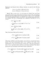
predicted and experimental results is presented in Figs. 3.35–3.37, where theoretical
dependencies of normalized moduli on the fiber volume fraction are shown with lines.
The dots correspond to the test data for epoxy composites reinforced with different fibers
Chapter 3. Mechanics of a unidirectional ply 93
0
0.2
0.4
0.6

0.8
0 0.2 0.4 0.6 0.8
E
1
E
f
v
f
Fig. 3.35. Dependence of the normalized longitudinal modulus on fiber volume fraction. zero-order
model, Eqs. (3.61);
first-order model, Eqs. (3.76);
•
experimental data.
0
2
4
6
8
10
0 0.2 0.4 0.6 0.8
E
2
v
f
E
m
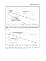
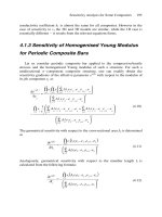
Fig. 3.36. Dependence of the normalized transverse modulus on fiber volume fraction.
first-order model,
Eq. (3.78);


second-order model, Eq. (3.89);
higher-order model (elasticity solution) (Van Fo Fy,
1966);
the upper bound;
•
experimental data.
94 Advanced mechanics of composite materials
0
2
4
6
8
10
0 0.2 0.4 0.6 0.8
G
12
G
m
v
f
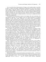
Fig. 3.37. Dependence of the normalized in-plane shear modulus on fiber volume fraction.
first-order
model, Eq. (3.81);

second-order model, Eq. (3.90);
higher-order model (elasticity solution)
(Van Fo Fy, 1966);
•
experimental data.
that have been measured by the authors or taken from publications of Tarnopol’skii and

Roze (1969), Kondo and Aoki (1982), and Lee et al. (1995). As can be seen in Fig. 3.35,
not only the first-order model, Eq. (3.76), but also the zero-order model, Eqs. (3.61),
provide fair predictions for E
1
, whereas Figs. 3.36 and 3.37 for E
2
and G
12
call for
an improvement to the first-order model (the corresponding results are shown with solid
lines).
Second-order models allow for the fiber shape and distribution, but, in contrast to
higher-order models, ignore the complicated stressed state in the fibers and matrix under
loading of the ply as shown in Fig. 3.29. To demonstrate this approach, consider a layer-
wise fiber distribution (see Fig. 3.5) and assume that the fibers are absolutely rigid and
the matrix is in the simplest uniaxial stressed state under transverse tension. The typical
element of this model is shown in Fig. 3.38, from which we can obtain the following
equation
v
f
=
πR
2
2Ra
=
πR
2a
(3.82)
Since 2R<a, v
f

< π/4 = 0.785. The equilibrium condition yields
2Rσ
2
=

R
−R
σ
m
dx
3
(3.83)
Chapter 3. Mechanics of a unidirectional ply 95
s
2
s
2
s
m
R
A
a
∆a
l(a)
x
2
x
3
1
2

3
A
a
Fig. 3.38. Microstructural model of the second order.
where x
3
= R cos α and σ
2
is some average transverse stress that induces average strain
ε
2
=
a
a
(3.84)
such that the effective (apparent) transverse modulus is calculated as
E
2
=
σ
2
ε
2
(3.85)
The strain in the matrix can be determined with the aid of Fig. 3.38 and Eq. (3.84), i.e.,
ε
m
=
a
l(α)

=
a
a −2R sin α
=
ε
2
1 −λ

1 −
(
x
3
/R
)
2
(3.86)
where, in accordance with Eq. (3.82),
λ =
2R
a
=
4v
f
π
(3.87)
Assuming that there is no strain in the matrix in the fiber direction and there is no stress
in the matrix in the x
3
direction, we have
σ

m
=
E
m
ε
m
1 −ν
2
m
(3.88)
96 Advanced mechanics of composite materials
Substituting σ
2
from Eq. (3.85) and σ
m
, from Eq. (3.88) into Eq. (3.83) and using Eq. (3.86)
to express ε
m
, we arrive at
E
2
=
E
m
2R

1 −ν
2
m



R
−R
dx
3
1 −λ

1 −x
2
3
Calculating the integral and taking into account Eq. (3.87), we finally get
E
2
=
πE
m
r(λ)
2v
f

1 −ν
2
m

(3.89)
where
r(λ) =
1
√
1 −λ

2
tan
−1

1 +λ
1 −λ
−
π
4
Similar derivation for an in-plane shear yields
G
12
=
πG
m
2v
f
r(λ) (3.90)
The dependencies of E
2
and G
12
on the fiber volume fraction corresponding to Eqs. (3.89)
and (3.90) are shown in Figs. 3.36 and 3.37 (dotted lines). As can be seen, the second-
order model of a ply provides better agreement with the experimental results than the
first-order model. This agreement can be further improved if we take a more realistic
microstructure of the material. Consider the actual microstructure shown in Fig. 3.2 and
single out a typical square element with size a as in Fig. 3.39. The dimension a should
provide the same fiber volume fraction for the element as for the material under study.
To calculate E

2
, we divide the element into a system of thin (h  a) strips parallel to
a
a
i
j
h
l
ij
x
2
x
3
Fig. 3.39. Typical structural element.
Chapter 3. Mechanics of a unidirectional ply 97
axis x
2
. The ith strip is shown in Fig. 3.39. For each strip, we measure the lengths, l
ij
,
of the matrix elements, the jth of which is shown in Fig. 3.39. Then, equations analogous
to Eqs. (3.83), (3.88), and (3.86) take the form
σ
2
a = h

i
σ
(i)
m

,σ
(i)
m
=
E
m
1 −ν
2
m
ε
(i)
m
,ε
(i)
m
=
ε
2
a

j
l
ij
and the final result is
E
2
=
E
m
h

1 −ν
2
m

i
⎛
⎝

j
l
ij
⎞
⎠
−1
where h = h/a, l
ij
= l
ij
/a. The second-order models considered above can be readily
generalized to account for the fiber transverse stiffness and matrix nonlinearity.
Numerous higher-order microstructural models and descriptive approaches have been
proposed, including
• analytical solutions in the problems of elasticity for an isotropic matrix having regular
inclusions – fibers or periodically spaced groups of fibers,
• numerical (finite element, finite difference methods) stress analysis of the matrix in the
vicinity of fibers,
• averaging of stress and strain fields for a media filled in with regularly or randomly
distributed fibers,
• asymptotic solutions of elasticity equations for inhomogeneous solids characterized by
a small microstructural parameter (fiber diameter),

• photoelasticity methods.
Exact elasticity solution for a periodical system of fibers embedded in an isotropic matrix
(Van Fo Fy (Vanin), 1966) is shown in Figs. 3.36 and 3.37. As can be seen, due to the
high scatter in experimental data, the higher-order model does not demonstrate significant
advantages with respect to elementary models.
Moreover, all the micromechanical models can hardly be used for practical analysis of
composite materials and structures. The reason for this is that irrespective of how rigorous
the micromechanical model is, it cannot describe sufficiently adequately real material
microstructure governed by a particular manufacturing process, taking into account voids,
microcracks, randomly damaged or misaligned fibers, and many other effects that cannot
be formally reflected in a mathematical model. As a result of this, micromechanical
models are mostly used for qualitative analysis, providing us with the understanding of
how material microstructural parameters affect the mechanical properties rather than with
quantitative information about these properties. Particularly, the foregoing analysis should
result in two main conclusions. First, the ply stiffness along the fibers is governed by the
fibers and linearly depends on the fiber volume fraction. Second, the ply stiffness across
the fibers and in shear is determined not only by the matrix (which is natural), but by the
fibers as well. Although the fibers do not take directly the load applied in the transverse
direction, they significantly increase the ply transverse stiffness (in comparison with the
stiffness of a pure matrix) acting as rigid inclusions in the matrix. Indeed, as can be seen
98 Advanced mechanics of composite materials
in Fig. 3.34, the higher the fiber fraction, a
f
, the lower the matrix fraction, a
m
, for the
same a, and the higher stress σ
2
should be applied to the ply to cause the same transverse
strain ε

2
because only matrix strips are deformable in the transverse direction.
Due to the aforementioned limitations of micromechanics, only the basic models were
considered above. Historical overview of micromechanical approaches and more detailed
description of the corresponding results can be found elsewhere (Bogdanovich and Pastore,
1996; Jones, 1999).
To analyze the foregoing micromechanical models, we used the traditional approach
based on direct derivation and solution of the system of equilibrium, constitutive, and
strain–displacement equations. Alternatively, the same problems can be solved with the aid
of variational principles discussed in Section 2.11. In their application to micromechanics,
these principles allow us not only to determine the apparent stiffnesses of the ply, but also
to establish the upper and the lower bounds on them.
Consider, for example, the problem of transverse tension of a ply under the action of
some average stress σ
2
(see Fig. 3.29) and apply the principle of minimum strain energy
(see Section 2.11.2). According to this principle, the actual stress field provides the value
of the body strain energy, which is equal to or less than that of any statically admissible
stress field. Equality takes place only if the admissible stress state coincides with the
actual one. Excluding this case, i.e., assuming that the class of admissible fields under
study does not contain the actual field, we can write the following strict inequality
W
adm
σ
>W
act
σ
(3.91)
For the problem of transverse tension, the fibers can be treated as absolutely rigid, and
only the matrix strain energy needs to be taken into account. We can also neglect the

energy of shear strain and consider the energy corresponding to normal strains only. With
due regard to these assumptions, we use Eqs. (2.51) and (2.52) to get
W =

V
m
UdV
m
(3.92)
where V
m
is the volume of the matrix, and
U =
1
2

σ
m
1
ε
m
1
+σ
m
2
ε
m
2
+σ
m

3
ε
m
3

(3.93)
To find energy W
σ
entering inequality (3.91), we should express strains in terms of stresses
with the aid of constitutive equations, i.e.,
ε
m
1
=
1
E
m

σ
m
1
−ν
m
σ
m
2
−ν
m
σ
m

3

ε
m
2
=
1
E
m

σ
m
2
−ν
m
σ
m
1
−ν
m
σ
m
3

(3.94)
ε
m
3
=
1

E
m

σ
m
3
−ν
m
σ
m
1
−ν
m
σ
m
2

Chapter 3. Mechanics of a unidirectional ply 99
Consider first the actual stress state. Let the ply in Fig. 3.29 be loaded with stress σ
2
inducing apparent strain ε
2
such that
ε
2
=
σ
2
E
act

2
(3.95)
Here, E
act
2
is the actual apparent modulus, which is not known. With due regard to
Eqs. (3.92) and (3.93) we get
W =
1
2
σ
2
ε
2
V, W
act
σ
=
σ
2
2
2E
act
2
V (3.96)
where V is the volume of the material. As an admissible field, we can take any state of
stress that satisfies the equilibrium equations and force boundary conditions. Using the
simplest first-order model shown in Fig. 3.34, we assume that
σ
m

1
= σ
m
3
= 0,σ
m
2
= σ
2
Then, Eqs. (3.92)–(3.94) yield
W
adm
σ
=
σ
2
2
2E
m
V
m
(3.97)
Substituting Eqs. (3.96) and (3.97) into the inequality (3.91), we arrive at
E
act
2
>E
l
2
where, in accordance with Eqs. (3.62) and Fig. 3.34,

E
l
2
=
E
m
V
V
m
=
E
m
v
m
This result, specifying the lower bound on the apparent transverse modulus, follows from
Eq. (3.78) if we put E
f
→∞. Thus, the lower (solid) line in Fig. 3.36 represents actually
the lower bound on E
2
.
To derive the expression for the upper bound, we should use the principle of minimum
total potential energy (see Section 2.11.1), according to which (we again assume that the
admissible field does not include the actual state)
T
adm
>T
act
(3.98)
where T = W

ε
− A. Here, W
ε
is determined with Eq. (3.92), in which stresses are
expressed in terms of strains with the aid of Eqs. (3.94), and A, for the problem under
study, is the product of the force acting on the ply and the ply extension induced by this
force. Since the force is the resultant of stress σ
2
(see Fig. 3.29), which induces strain ε
2
,
100 Advanced mechanics of composite materials
and same for actual and admissible states, A is also the same for both states, and we can
present inequality (3.98) as
W
adm
ε
>W
act
ε
(3.99)
For the actual state, we can write equations similar to Eqs. (3.96), i.e.,
W =
1
2
σ
2
ε
2
V, W

act
ε
=
1
2
E
act
2
ε
2
2
V (3.100)
in which V = 2Ra in accordance with Fig. 3.38. For the admissible state, we use the
second-order model (see Fig. 3.38) and assume that
ε
m
1
= 0,ε
m
2
= ε
m
,ε
m
3
= 0
where ε
m
is the matrix strain specified by Eq. (3.86). Then, Eqs. (3.94) yield
σ

m
1
= µ
m
σ
m
2
,σ
m
3
= µ
m
σ
m
2
,σ
m
2
=
E
m
ε
m
1 −2ν
m
µ
m
(3.101)
where
µ

m
=
ν
m
(1 +ν
m
)
1 −ν
2
m
Substituting Eqs. (3.101) into Eq. (3.93) and performing integration in accordance with
Eq. (3.92), we have
W
adm
ε
=
E
m
ε
2
2
1 −2ν
m
µ
m
·

R
−R
dx

3

a
2
y
0
dx
2
y
2
=
πRaE
m
ε
2
2
r(λ)
2v
f
(1 −2ν
m
µ
m
)
(3.102)
Here,
y = 1 −λ

1 −


x
3
R

2
and r(λ) is given above; see also Eq. (3.89). Applying Eqs. (3.100) and (3.102) in
conjunction with inequality (3.99), we arrive at
E
act
2
<E
u
2
where
E
u
2
=
πE
m
2v
f
(1 −2ν
m
µ
m
)
is the upper bound on E
2
shown in Fig. 3.36 with a dashed curve.

Chapter 3. Mechanics of a unidirectional ply 101
Taking statically and kinematically admissible stress and strain fields that are closer to
the actual states of stress and strain, one can increase E
l
2
and decrease E
u
2
, making the
difference between the bounds smaller (Hashin and Rosen, 1964).
It should be emphasized that the bounds established thus are not the bounds imposed
on the modulus of a real composite material but on the result of calculation corresponding
to the accepted material model. Indeed, we can return to the first-order model shown in
Fig. 3.34 and consider in-plane shear with stress τ
12
. As can be readily proved, the actual
stress–strain state of the matrix in this case is characterized with the following stresses
and strains
σ
m
1
= σ
m
2
= σ
m
3
= 0,τ
m
12

= τ
12
,τ
m
13
= τ
m
23
= 0,
ε
m
1
= ε
m
2
= ε
m
3
= 0,γ
m
12
= γ
12
,γ
m
13
= γ
m
23
= 0

(3.103)
Assuming that the fibers are absolutely rigid and considering stresses and strains in
Eqs. (3.103) as statically and kinematically admissible, we can readily find that
G
act
12
= G
l
12
= G
u
12
=
G
m
v
m
Thus, we have found the exact solution, but its agreement with experimental data is rather
poor (see Fig. 3.37) because the material model is not sufficiently adequate.
As follows from the foregoing discussion, micromechanical analysis provides only
qualitative prediction of the ply stiffness. The same is true for ply strength. Although
the micromechanical approach, in principle, can be used for strength analysis (Skudra
et al., 1989), it provides mainly better understanding of the failure mechanism rather
than the values of the ultimate stresses for typical loading cases. For practical appli-
cations, these stresses are determined by experimental methods described in the next
section.
3.4. Mechanical properties of a ply under tension, shear, and compression
As is shown in Fig. 3.29, a ply can experience five types of elementary loading, i.e.,
• tension along the fibers,
• tension across the fibers,

• in-plane shear,
• compression along the fibers,
• compression across the fibers.
Actual mechanical properties of a ply under these loading cases are determined experi-
mentally by testing specially fabricated specimens. Since the thickness of an elementary
ply is very small (0.1–0.02 mm), the specimen usually consists of tens of plies having the
same fiber orientations.
Mechanical properties of composite materials depend on the processing method and
parameters. So, to obtain the adequate material characteristics that can be used for analysis
of structural elements, the specimens should be fabricated by the same processes that are
102 Advanced mechanics of composite materials
Table 3.5
Typical properties of unidirectional composites.
Property Glass–
epoxy
Carbon–
epoxy
Carbon–
PEEK
Aramid–
epoxy
Boron–
epoxy
Boron–
Al
Carbon–
Carbon
Al
2
O

3
–
Al
Fiber volume fraction, v
f
0.65 0.62 0.61 0.6 0.5 0.5 0.6 0.6
Density, ρ (g/cm
3
) 2.1 1.55 1.6 1.32 2.1 2.65 1.75 3.45
Longitudinal modulus,
E
1
(GPa)
60 140 140 95 210 260 170 260
Transverse modulus, E
2
(GPa)
13 11 10 5.1 19 140 19 150
Shear modulus, G
12
(GPa)
3.4 5.5 5.1 1.8 4.8 60 9 60
Poisson’s ratio, ν
21
0.3 0.27 0.3 0.34 0.21 0.3 0.3 0.24
Longitudinal tensile
strength,
σ
+
1

(MPa)
1800 2000 2100 2500 1300 1300 340 700
Longitudinal compressive
strength,
σ
−
1
(MPa)
650 1200 1200 300 2000 2000 180 3400
Transverse tensile
strength,
σ
+
2
(MPa)
40 50 75 30 70 140 7 190
Transverse compressive
strength,
σ
−
2
(MPa)
90 170 250 130 300 300 50 400
In-plane shear strength,
τ
12
(MPa)
50 70 160 30 80 90 30 120
used to manufacture the structural elements. In connection with this, there exist two
standard types of specimens – flat ones that are used to test materials made by hand or

machine lay-up and cylindrical (tubular or ring) specimens that represent materials made
by winding.
Typical mechanical properties of unidirectional advanced composites are presented in
Table 3.5 and in Figs. 3.40–3.43. More data relevant to the various types of particular
composite materials could be found in Peters (1998).
We now consider typical loading cases.
3.4.1. Longitudinal tension
Stiffness and strength of unidirectional composites under longitudinal tension are deter-
mined by the fibers. As follows from Fig. 3.35, material stiffness linearly increases with
increase in the fiber volume fraction. The same law following from Eq. (3.75) is valid for
the material strength. If the fiber’s ultimate elongation,
ε
f
, is less than that of the matrix
(which is normally the case), the longitudinal tensile strength is determined as
σ
+
1
= (E
f
v
f
+E
m
v
m
)ε
f
(3.104)
However, in contrast to Eq. (3.76) for E

1
, this equation is not valid for very small and very
high fiber volume fractions. The dependence of
σ
+
1
on v
f
is shown in Fig. 3.44. For very
Chapter 3. Mechanics of a unidirectional ply 103
0
400
800
1200
1600
2000
0
s
1
, MPa
(a)
e
2
; g
12
, %
0
30
60
90

024
s
2
; τ
12
, MPa
s
2
–
s
2
+
t
12
(b)
531
321
e
1
, %
s
+
1
s
1
–
Fig. 3.40. Stress–strain curves for unidirectional glass–epoxy composite material under longitudinal tension and
compression (a), transverse tension and compression (b), and in-plane shear (b).
low v
f

, the fibers do not restrain the matrix deformation. Being stretched by the matrix,
the fibers fail because their ultimate elongation is less than that of the matrix and the
induced stress concentration in the matrix can reduce material strength below the strength
of the matrix (point B). Line BC in Fig. 3.44 corresponds to Eq. (3.104). At point C, the
amount of the matrix reduces below the level necessary for a monolithic material, and the
material strength at point D approximately corresponds to the strength of a dry bundle
of fibers, which is less than the strength of a composite bundle of fibers bound with the
matrix (see Table 3.3).
Strength and stiffness under longitudinal tension are determined using unidirectional
strips or rings. The strips are cut out of unidirectionally reinforced plates, and their ends
are made thicker (usually glass–epoxy tabs are bonded onto the ends) to avoid specimen
104 Advanced mechanics of composite materials
0
400
800
1200
1600
2000
01
(a)
0
50
100
150
200
02
(b)
s
1
, MPa

e
1
, %
1.5
s
2
–
s
2
+
e
2
; g
12
, %
s
2
; τ
12
, MPa
0.5
31
t
12
s
+
1
s
1
–

Fig. 3.41. Stress–strain curves for unidirectional carbon–epoxy composite material under longitudinal tension
and compression (a), transverse tension and compression (b), and in-plane shear (b).
failure in the grips of the testing machine (Jones, 1999; Lagace, 1985). Rings are cut
out of a circumferentially wound cylinder or wound individually on a special mandrel, as
shown in Fig. 3.45. The strips are tested using traditional approaches, whereas the rings
should be loaded with internal pressure. There exist several methods to apply the pressure
Chapter 3. Mechanics of a unidirectional ply 105
0
400
800
1200
1600
2000
2400
2800
0 0.5 1 1.5 2 2.5 3
(a)
0
50
100
150
0
(b)
s
1
, MPa
e
1
, %
321

e
2
; g
12
, %
s
2
; τ
12
, MPa
s
2
–
s
2
+
t
12
s
+
1
s
1
–
Fig. 3.42. Stress–strain curves for unidirectional aramid–epoxy composite material under longitudinal tension
and compression (a), transverse tension and compression (b), and in-plane shear (b).
(Tarnopol’skii and Kincis, 1985), the simplest of which involves the use of mechanical
fixtures with various numbers of sectors as in Figs. 3.46 and 3.47. The failure mode is
shown in Fig. 3.48. Longitudinal tension yields the following mechanical properties of the
material

• longitudinal modulus, E
1
,
• longitudinal tensile strength,
σ
+
1
,
• Poisson’s ratio, ν
21
.
106 Advanced mechanics of composite materials
0
400
800
1200
1600
2000
2400
0 0.4 0.8 1.2 1.6
(a)
0
100
200
300
0
(b)
s
1
, MPa

e
2
; g
12
, %
s
2
; τ
12
, MPa
e
1
, %
321
s
2
–
s
2
+
t
12
s
+
1
s
1
–
Fig. 3.43. Stress–strain curves for unidirectional boron–epoxy composite material under longitudinal tension
and compression (a), transverse tension and compression (b), and in-plane shear (b).

Typical values of these characteristics for composites with various fibers and matrices are
listed in Table 3.5. It follows from Figs. 3.40–3.43, that the stress–strain diagrams are
linear practically up to failure.
3.4.2. Transverse tension
There are three possible modes of material failure under transverse tension with stress
σ
2
shown in Fig. 3.49 – failure of the fiber–matrix interface (adhesion failure), failure
Chapter 3. Mechanics of a unidirectional ply 107
0
0.2
0.4
0.6
0.8
1
0 0.2 0.4 0.6 0.8
v
f
C
D
B
A
s
1
+
Fig. 3.44. Dependence of normalized longitudinal strength on fiber volume fraction ( – experimental results).
Fig. 3.45. A mandrel for test rings.
108 Advanced mechanics of composite materials
Fig. 3.46. Two-, four-, and eight-sector test fixtures for composite rings.
Fig. 3.47. A composite ring on a eight-sector test fixture.

Fig. 3.48. Failure modes of unidirectional rings.
Chapter 3. Mechanics of a unidirectional ply 109
1
2
3
s
2
s
2
Fig. 3.49. Modes of failure under transverse tension: 1 – adhesion failure; 2 – cohesion failure; 3 – fiber failure.
of the matrix (cohesion failure), and fiber failure. The last failure mode is specific for
composites with aramid fibers, which consist of thin filaments (fibrils) and have low
transverse strength. As follows from the micromechanical analysis (Section 3.3), material
stiffness under tension across the fibers is higher than that of a pure matrix (see Fig. 3.36).
For qualitative analysis of transverse strength, consider again the second-order model in
Fig. 3.38. As can be seen, the stress distribution σ
m
(x
3
) is not uniform, and the maximum
stress in the matrix corresponds to α = 90
◦
. Using Eqs. (3.85), (3.86), and (3.88), we
obtain
σ
max
m
=
E
m

σ
2

1 −ν
2
m

E
2
(1 −λ)
Taking σ
max
m
= σ
m
and σ
2
= σ
+
2
, where σ
m
and σ
+
2
are the ultimate stresses for the matrix
and composite material, respectively, and substituting for λ and E
2
their expressions in
accordance with Eqs. (3.87) and (3.89), we arrive at

σ
+
2
= σ
m
r(λ)
2v
f
(π −4v
f
) (3.105)
The variation of the ratio
σ
+
2
/σ
m
for epoxy composites is shown in Fig. 3.50. As can be
seen, the transverse strength of a unidirectional material is considerably lower than the
strength of the matrix. It should be noted that for the first-order model, which ignores the
shape of the fiber cross sections (see Fig. 3.34),
σ
+
2
is equal to σ
m
. Thus, the reduction
of
σ
+

2
is caused by stress concentration in the matrix induced by cylindrical fibers.
However, both polymeric and metal matrices exhibit, as follows from Figs. 1.11 and
1.14, elastic–plastic behavior, and it is known that plastic deformation reduces the effect of
stress concentration. Nevertheless, the stress–strain diagrams
σ
+
2
–ε
2
, shown in Figs. 3.40–
3.43, are linear up to the failure point. To explain this phenomenon, consider element A
of the matrix located in the vicinity of a fiber as in Fig. 3.38. Assuming that the fiber is
absolutely rigid, we can conclude that the matrix strains in directions 1 and 3 are close to
zero. Taking ε
m
1
= ε
m
3
= 0 in Eqs. (3.94), we arrive at Eqs. (3.101) for stresses, according
to which σ
m
1
= σ
m
3
= µ
m
σ

m
2
. The dependence of parameter µ
m
on the matrix Poisson’s
110 Advanced mechanics of composite materials
0
0.2
0.4
0.6
0.8
1
0 0.2 0.4 0.6 0.8
+
s
m
s
2
v
f
Fig. 3.50. Dependence of material strength under transverse tension on fiber volume fraction:
(
) Eq. (3.105); (
•
) experimental data.
ratio is presented in Fig. 3.51. As follows from this figure, in the limiting case ν
m
= 0.5,
we have µ
m

= 1 and σ
m
1
= σ
m
2
= σ
m
3
, i.e., the state of stress under which all the materials
behave as absolutely brittle. For epoxy resin, ν
m
= 0.35 and µ
m
= 0.54, which, as can be
supposed, does not allow the resin to demonstrate its rather limited (see Fig. 1.11) plastic
properties.
Strength and stiffness under transverse tension are experimentally determined using
flat strips (see Fig. 3.52) or tubular specimens (see Fig. 3.53). These tests allow us to
determine
• transverse modulus, E
2
,
• transverse tensile strength,
σ
+
2
.
For typical composite materials, these properties are given in Table 3.5.
3.4.3. In-plane shear

The failure modes in unidirectional composites under in-plane pure shear with stress τ
12
shown in Fig. 3.29 are practically the same as those for the case of transverse tension
(see Fig. 3.49). However, there is a significant difference in material behavior. As follows
from Figs. 3.40–3.43, the stress–strain curves τ
12
−γ
12
are not linear, and τ
12
exceeds σ
+
2
.
Chapter 3. Mechanics of a unidirectional ply 111
0.3
0.4
0.5
0.6
0.7
0.8
0.9
1
0.3 0.35 0.4 0.45 0.5
m
m
u
m
Fig. 3.51. Dependence of parameter µ
m

on the matrix Poisson’s ratio.
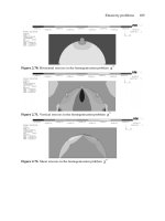
Fig. 3.52. Test fixture for transverse tension and compression of unidirectional strips.
This means that the fibers do not restrict the free shear deformation of the matrix, and the
stress concentration in the vicinity of the fibers does not significantly influence material
strength because of matrix plastic deformation.
Strength and stiffness under in-plane shear are determined experimentally by testing
plates and thin-walled cylinders. A plate is reinforced at 45
◦
to the loading direction and
Fig. 3.53. Test fixture for transverse tension or compression of unidirectional tubular specimens.
P
P
a
t
12
x
y
1
2
45°
Fig. 3.54. Simulation of pure shear in a square frame.
Chapter 3. Mechanics of a unidirectional ply 113
Fig. 3.55. A tubular specimen for shear test.
is fixed in a square frame consisting of four hinged members, as shown in Fig. 3.54.
Simple equilibrium consideration and geometric analysis with the aid of Eq. (2.27) yield
the following equations
τ
12
=
P

√
2ah
,γ
12
= ε
y
−ε
x
,G
12
=
τ
12
γ
12
in which h is the plate thickness. Thus, knowing P and measuring strains in the x and
y directions, we can determine
τ
12
and G
12
. More accurate and reliable results can be
obtained if we induce pure shear in a twisted tubular specimen reinforced in the circum-
ferential direction (Fig. 3.55). Again, using simple equilibrium and geometric analysis,
we get
τ
12
=
M
2πR

2
h
,γ
12
=
ϕR
l
,G
12
=
τ
12
γ
12
Here, M is the torque, R and h are the cylinder radius and thickness, and ϕ is the
twist angle between two cross-sections located at some distance l from each other. Thus,
knowing M and measuring ϕ, we can find
τ
12
and G
12
.
3.4.4. Longitudinal compression
Failure under compression along the fibers can occur in different modes, depending on
the material microstructural parameters, and can hardly be predicted by micromechanical
analysis because of the rather complicated interaction of these modes. Nevertheless, useful
qualitative results allowing us to understand material behavior and, hence, to improve
properties, can be obtained with microstructural models.
114 Advanced mechanics of composite materials
s

1
s
1
t
t
a
Fig. 3.56. Shear failure under compression.
Consider typical compression failure modes. The usual failure mode under compression
is associated with shear in some oblique plane as in Fig. 3.56. The shear stress can be
calculated using Eq. (2.9), i.e.,
τ = σ
1
sin α cos α
and reaches its maximum value at α = 45
◦
. Shear failure under compression is usually typ-
ical for unidirectional composites that demonstrate the highest strength under longitudinal
compression. On the other hand, materials showing the lowest strength under compres-
sion exhibit a transverse extension failure mode typical of wood compressed along the
fibers, and is shown in Fig. 3.57. This failure is caused by tensile transverse strain, whose
absolute value is
ε
2
= ν
21
ε
1
(3.106)
where ν
21

is Poisson’s ratio and ε
1
= σ
1
/E
1
is the longitudinal strain. Consider Table 3.6,
showing some data taken from Table 3.5 and the results of calculations for epoxy compos-
ites. The fourth column displays the experimental ultimate transverse strains
ε
+
2
= σ
+
2
/E
2
s
1
s
1
1
2
Fig. 3.57. Transverse extension failure mode under longitudinal compression.
Table 3.6
Characteristics of epoxy composites.
Material Characteristic
σ
−
1

(MPa) ε
−
1
(%) ν
21
ε
+
2
(%) ε
2
= ν
21
ε
−
1
Glass–epoxy 600 1.00 0.30 0.31 0.30
Carbon–epoxy 1200 0.86 0.27 0.45 0.23
Aramid–epoxy 300 0.31 0.34 0.59 0.11
Boron–epoxy 2000 0.95 0.21 0.37 0.20
Chapter 3. Mechanics of a unidirectional ply 115
0
5
10
15
20
25
0 0.2 0.4 0.6 0.8
k
e
v

f
Fig. 3.58. Dependence of strain concentration factor on the fiber volume fraction.
calculated with the aid of data presented in Table 3.5, whereas the last column shows the
results following from Eq. (3.106). As can be seen, the failure mode associated with
transverse tension under longitudinal compression is not dangerous for the composites
under consideration because
ε
+
2
> ε
2
. However, this is true only for fiber volume frac-
tions v
f
= 0.50−0.65, to which the data presented in Table 3.6 correspond. To see what
happens for higher fiber volume fractions, let us use the second-order micromechanical
model and the corresponding results in Figs. 3.36 and 3.50. We can plot the strain con-
centration factor k
ε
(which is the ratio of the ultimate matrix elongation, ε
m
,toε
+
2
for
the composite material) versus the fiber volume fraction. As can be seen in Fig. 3.58, this
factor, being about 6 for v
f
= 0.6, becomes as high as 25 for v
f

= 0.75. This means
that
ε
+
2
dramatically decreases for higher v
f
, and the fracture mode shown in Fig. 3.57
becomes quite usual for composites with high fiber volume fractions.
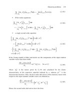
Both fracture modes shown in Figs. 3.56 and 3.57 are accompanied with fibers bending
induced by local buckling of fibers. According to N.F. Dow and B.W. Rosen (Jones, 1999),
there can exist two modes of fiber buckling, as shown in Fig. 3.59 – a shear mode and
a transverse extension mode. To study the fiber’s local buckling (or microbuckling, which
means that the material specimen is straight, whereas the fibers inside the material are
curved), consider a plane model of a unidirectional ply, shown in Figs. 3.15 and 3.60, and
take a
m
= a and a
f
= δ = d, where d is the fiber diameter. Then, Eqs. (3.17) yield
v
f
=
d
1 +d
,
d =
d
a
(3.107)

116 Advanced mechanics of composite materials
(a) (b)
Fig. 3.59. Shear (a) and transverse extension (b) modes of fiber local buckling.
s
1
s
1

1
2
y, u
y
x, u
x
c
a
d
v
1
(x)
v
2
(x)
l
n
a
Fig. 3.60. Local buckling of fibers in unidirectional ply.
Because of the symmetry conditions, consider two fibers 1 and 2 in Fig. 3.60 and the
matrix between these fibers. The buckling displacement, v, of the fibers can be represented
with a sine function as

v
1
(x) = V sin λ
n
x, v
2
(x) = V sin λ
n
(x −c) (3.108)
where V is an unknown amplitude value, the same for all the fibers, λ
n
= π/l
n
, l
n
is
a half of a fiber wavelength (see Fig. 3.60), and c = (a + d)cot α is a phase shift.
Taking c = 0, we can describe the shear mode of buckling (Fig. 3.59(a)), whereas c = l
n
corresponds to the extension mode (Fig. 3.59(b)). To find the critical value of stress σ
1
,we
use the Timoshenko energy method (Timoshenko and Gere, 1961), yielding the following
buckling condition
A = W (3.109)
Here, A is the work of external forces, and W is the strain energy accumulated in the
material while the fibers undergo buckling. Work A and energy W are calculated for a
typical ply element consisting of two halves of fibers 1 and 2 and the matrix between