CHAPTER 5
Fundamentals of Engineered
Environmental Systems
CHAPTER PREVIEW
Applications of the fundamentals of transport processes and reactions
in developing material balance equations for engineered environmen-
tal systems are reviewed in this chapter. Alternate reactor configura-
tions involving homogeneous and heterogeneous systems with solid,
liquid, and gas phases are identified. Models to describe the perform-
ances of selected reactor configurations under nonflow, flow, steady,
and unsteady conditions are developed. The objective here is to pro-
vide the background for the modeling examples to be presented in
Chapter 8.
5.1 INTRODUCTION
C
HAPTER
4 contained a review of environmental processes and reactions.
In this chapter, their application to engineered systems is reviewed. An
engineered environmental system is defined here as a unit process, operation,
or system that is designed, optimized, controlled, and operated to achieve
transformation of materials to prevent, minimize, or remedy their undesired
impacts on the environment.
The application and analysis of environmental processes and reactions in
engineered systems follow the well-established practice of reaction engineer-
ing in the field of chemical engineering. While both chemical and environ-
mental systems deal with processes and reactions involving liquids, solids,
and gases, some important differences between the two systems have to be
noted. Environmental systems are often more complex than chemical sys-
tems, and therefore, several simplifying assumptions have to be made in
Chapter 05 11/9/01 11:23 AM Page 105
© 2002 by CRC Press LLC

analyzing and modeling them. The exact composition and nature of the
inflows are well defined in chemical systems, whereas in environmental sys-
tems, lumped surrogate measures are used (e.g., BOD, COD, coliform). The
flow rates are often constant, steady, or predictable in chemical systems,
whereas, in environmental systems, they are not, as a rule.
Engineered environmental systems are built up of reactors. A reactor is
defined here as any device in which materials can undergo chemical, biochem-
ical, biological, or physical processes resulting in chemical transformations,
phase changes, or separations. The starting point in developing mathematical
models of such reactors and systems is the material balance (MB). Principles
of micro- and macro-transport theory and process/reaction kinetics (reviewed
in Chapter 4) can be applied to derive expressions for inflows, outflows, and
transformations to complete the MB equation. The mathematical form of the
final MB equation can be algebraic or differential, depending on the nature of
flows, reactions, and the type of reactor.
A complete analysis of reactors is beyond the scope of this book, and read-
ers should refer to other specific texts on reactor engineering for further
details. Excellent examples of such texts include those by Webber (1972),
Treybal (1980), Levenspiel (1972), and Weber and DiGiano (1996).
5.2 CLASSIFICATIONS OF REACTORS
Reactors can be classified into several different types for the purposes of
analysis and modeling. At the outset, they can be classified based on the type
of flow and extent of mixing through the reactor. These factors determine the
amount of time spent by the material inside the reactor, which, in turn, deter-
mines the extent of reaction undergone by the material. At one extreme con-
dition, complete mixing of all elements within the reactor occurs; and at the
other extreme, no mixing whatsoever occurs. The former type of reactors is
referred to as completely mixed reactors and the latter, as plug flow reactors.
Complete mixing here implies that concentration gradients do not exist
within the reactor, and the reaction rate is the same everywhere inside the

reactor. A corollary of this condition is that the concentration in the effluent
of a completely mixed reactor is equal to that inside the reactor. In contrast,
plug flow reactors are characterized by concentration gradients, therefore,
they have spatially varying reaction rates within the reactor. Thus, completely
mixed reactors fall under lumped systems, and plug flow reactors fall under
distributed systems.
Reactors with either complete mixing on one extreme or no mixing on the
other extreme are known as ideal reactors. Reactors in which some interme-
diate degree of mixing between the two extremes occurs are called nonideal
Chapter 05 11/9/01 11:23 AM Page 106
© 2002 by CRC Press LLC
reactors. While most reactors are analyzed and designed to be ideal, in prac-
tice, all reactors exhibit some degree of nonideality due to channeling, short-
circuiting, stagnant regions, inlet/outlet effects, wall effects, etc. The degree
of nonideality can be quantified through residence time distribution (RTD)
studies. Even the best-designed reactors often exhibit some degree of non-
ideality that requires complex models; hence, they are often approximated by
modified ideal reactors. For example, large, nonideal continuous mixed-flow
reactors (CMFRs) can be approximated by smaller, ideal CMFRs operating in
series; large nonideal plug flow reactors (PFRs) may be approximated by
ideal PFRs with dispersive transport added on. Thus, it is beneficial to fully
appreciate ideal reactors and develop models for them so that large, full-scale
reactors could be realistically designed, operated, and evaluated.
Ideal reactors can be further divided into homogeneous vs. heterogeneous,
depending on the number of phases involved; flow vs. nonflow, depending on
whether or not the flow of material occurs during the reaction; or steady vs.
unsteady, depending on the time-dependency of the parameters. Illustrative
applications of the fundamentals of environmental processes in homogeneous
and heterogeneous reactors under flow, nonflow, steady, and unsteady condi-
tions are presented in the following sections.

5.2.1 HOMOGENEOUS REACTORS
Homogeneous reactors entail reactions within one phase. Classification of
some of the common homogeneous reactors is shown in Table 5.1.
The MB equation forms the basis for analyzing and modeling reactors. In
the case of homogeneous reactors, bulk fluid flow characteristics and reaction
kinetics at the macroscopic or reactor scale are primary factors to consider.
Completely
Mixed
Batch
Reactors
(CMBR)
Sequencing
Batch
Reactors
(SBR)
Completely
Mixed Fed
Batch
Reactors
(CMFBR)
Completely
Mixed Flow
Reactors
(CMFR)
Plug Flow
Reactors
(PFR)
With
recycle
Without

recycle
Non-flow Reactors
Homogeneous Reactors
Flo Reactors
Nonflow Reactors
Flow Reactors
Table 5.1 Classification of Homogeneous Reactors
Chapter 05 11/9/01 11:23 AM Page 107
© 2002 by CRC Press LLC
5.2.2 HETEROGENEOUS REACTORS
Heterogeneous reactors entail reactions within two or more different
phases such as gas-liquid, gas-solid, and liquid-solid systems. Classification
of heterogeneous reactors commonly used in environmental studies is shown
in Table 5.2.
While transport at the macro and reactor scales and reaction rates are
the significant factors in homogeneous systems, micro- and macro-transport
scales and inter- and intraphase mass transfer processes are significant in
heterogeneous systems. As such, hydraulic retention times and reaction rate
constants characterize homogeneous systems, and reaction rates and mass
transfer coefficients characterize heterogeneous systems. The amounts of
interfacial surface areas and path lengths for intraphase transport as well as
bulk fluid dynamics contribute to the effectiveness of various heterogeneous
reactor configurations.
5.3 MODELING OF HOMOGENEOUS REACTORS
In the following sections, development of the MB equation for various
configurations of homogeneous reactors is summarized. The goal of this sec-
tion is not to provide a formal treatment of reactor engineering, but instead to
illustrate the different forms of MB equations, mathematical formulations,
and the solution procedures that are involved in the modeling of common
engineered environmental reactors.

\
Table 5.2
Classification of Heterogeneous Reactors
Chapter 05 11/9/01 11:23 AM Page 108
© 2002 by CRC Press LLC
5.3.1 COMPLETELY MIXED BATCH REACTORS
In completely mixed batch reactors (CMBRs), the reactor is first charged
with the reactants, and the products are discharged after completion of the
reactions. During the reaction, inflow and outflow are zero, and the volume,
V (L
3
), remains constant, but the concentration of the material undergoing the
reaction changes with time, starting at an initial value of C
0
. The MB equa-
tion for a CMBR during the reaction is as follows:
ᎏ
d(V
dt
C)
ᎏ
= –rV = –kCV (5.1)
where r is the rate of removal of the material by reactions (ML
–3
T
–1
), and k
is the first-order reaction rate constant (T
–1
). The solution to the MB equation

is as follows:
C = C
0
e
–kt
(5.2)
or
t = –
ᎏ
1
k
ᎏ
ln
΂
ᎏ
C
C
0
ᎏ
΃
(5.3)
where C is the concentration of the material at any time, t, during the reaction.
5.3.2 SEQUENCING BATCH REACTOR
In sequencing batch reactors (SBRs), a sequence of processes can take
place in the same reactor in a cyclic manner, typically starting with a fill
phase. Reaction can occur during the fill phase of the cycle as the volume
increases and can continue at constant volume after completion of the fill
phase. On completion of the reaction, another process can take place, or the
contents can be decanted to complete the cycle. The volume, V
t

, at any time,
t, during the fill phase = V
0
+ Qt, where V
0
is the volume remaining in the
reactor at the beginning of the fill phase (i.e., t = 0), and Q is the volumetric
fill rate (L
3
T
–1
). The MB equation during the fill phase, with reaction, for
example, is as follows:
ᎏ
d(V
dt
t
C)
ᎏ
= rV
t
ϩ QC
in
= –kCV
t
ϩ QC
in
(5.4)
which can be expanded to:
ᎏ

d
d
t
ᎏ
[(V
0
ϩ Qt)C] = –kC(V
0
ϩ Qt) ϩ QC
in
(5.5)
The solution to the above MB equation is:
Chapter 05 11/9/01 11:23 AM Page 109
© 2002 by CRC Press LLC
Figure 5.1 Concentration profile in an SBR during the fill phase.
C =
ᎏ
(t ϩ
C
in
t
0
)k
ᎏ
–
΄
ᎏ
C
t
0

i
k
n
ᎏ
– C
0
΅
ᎏ
(t ϩ
t
0
t
0
)
ᎏ
e
–kt
(5.6)
where t
0
= V
0
/Q and C
0
is the concentration remaining in the reactor at t = 0.
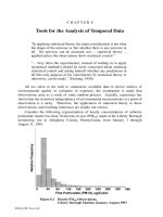
While the final result is difficult to interpret in the above form, a plot of C vs.
t can provide more insight into the dynamics of the process. An Excel
®
model
of the process is presented in Figure 5.1. A complete model for a biological

SBR with Michaelis-Menten type reaction kinetics is detailed in Chapter 8,
where the profiles of COD, dissolved oxygen, and biomass are developed
employing three coupled differential equations.
5.3.3 COMPLETELY MIXED FLOW REACTORS
Completely mixed flow reactors (CMFRs) are completely mixed with
continuous inflow and outflow. CMFRs are, by far, the most common environ-
mental reactors and are often operated under steady state conditions,
i.e., d( )/dt = 0. Under such conditions, the inflow should equal the outflow, while
the active reactor volume, V, remains constant. A key characteristic of CMFRs is
that the effluent concentration is the same as that inside the reactor. CMFRs can
Chapter 05 11/9/01 11:23 AM Page 110
© 2002 by CRC Press LLC
be characterized by their detention time, τ, or the hydraulic residence time (HRT),
which is given by τ = HRT = V/Q. The material balance equation is as follows:
ᎏ
d(V
dt
C)
ᎏ
= rV + QC
in
– QC (5.7)
which at steady state reduces to:
0 = –kCV ϩ QC
in
– QC (5.8)
whose solution is:
C =
ᎏ
Q

Q
ϩ
C
i
k
n
V
ᎏ
= ϭ
ᎏ
1
C
+
in
kτ
ᎏ
(5.9)
In some instances, multiple CMFRs are used in series, as shown in Figure 5.2,
to represent a single nonideal reactor, or to improve overall performance, or
to minimize total reactor volume.
For n such identical CMFRs shown in Figure 5.2, the overall concentration
ratio is related to the individual ratio of each reactor by the following
series:
ᎏ
C
C
ou
in
t,n
ᎏ

=
΂
ᎏ
C
C
i
1
n
ᎏ
΃
×
΂
ᎏ
C
C
2
1
ᎏ
΃
× . . .
΂
ᎏ
C
C
o
n
u
–
t
1

,n
ᎏ
΃
(5.10)
where C
p
is the effluent concentration of the pth reactor (p = 1 to n).
Substituting from the result found above for a single CMFR into the above
series gives the following:
ᎏ
C
C
ou
in
t,n
ᎏ
=
΂
ᎏ
1+
1
kτ
ᎏ
΃
n
or, overall, τ = n
Ά·
(5.11)
΄
ᎏ

C
C
ou
in
t,n
ᎏ
΅
1/n
– 1
ᎏᎏ
k
C
in
ᎏᎏ
1 + k
΂
ᎏ
Q
V
ᎏ
΃
Figure 5.2 CMFRs in series.
Q, Cin Q, C1 Q, C2
Q, Cout,n
Reactor 1 Reactor 2
Reactor n
Q, Cin
Q, C1 Q, C2
Q, Cout,n
Chapter 05 11/9/01 11:23 AM Page 111

© 2002 by CRC Press LLC
Worked Example 5.1
A wastewater treatment system for a rural community consists of two
completely mixed lagoons in series, the first one of HRT = 10 days, and the
second one of HRT = 5 days. It is desired to check whether this system can
meet a newly introduced regulation of 99.9% reduction of fecal coliform by
a first-order die off. The rate constant, k, for the die-off reaction has been
found to be a function of HRT described by k = 0.2τ – 0.3 (adapted from
Weber and DiGiano, 1996).
Solution
Because Equation (5.11) assumes identical rate constants in all the reac-
tors, it cannot be applied here. However, Equations (5.9) and (5.10) can be
applied to yield the following:
ᎏ
C
C
2,
i
o
n
ut
ᎏ
=
΂
ᎏ
C
C
i
1
n

ᎏ
΃΂
ᎏ
C
C
2,o
1
ut
ᎏ
΃
=
΂
ᎏ
1 ϩ
1
k
1
τ
1
ᎏ
΃΂
ᎏ
1 ϩ
1
k
2
τ
2
ᎏ
΃

Substituting the given data of: τ
1
= 10 days, τ
2
= 5 days, k
1
= 0.2 * 10 – 0.3 = 1.7,
and k
2
= 0.2 * 5 – 0.3 = 0.7,
ᎏ
C
C
2,
i
o
n
ut
ᎏ
=
΂
ᎏ
1+(1
1
.7)(10)
ᎏ
΃΂
ᎏ
1+(0
1

.7)(5)
ᎏ
΃
= 0.0123
and, hence, the percent reduction that can be achieved is 98.77%, which is
less than the target of 99.9%.
One option for meeting the new standard is to construct a third lagoon in
series. Its detention time can be determined as follows to achieve a reduction
of 99.9%, or an overall concentration ratio of 0.001:
ᎏ
C
C
3,
i
o
n
ut
ᎏ
= 0.001 =
Ά΂
ᎏ
C
C
i
1
n
ᎏ
΃΂
ᎏ
C

C
2
1
ᎏ
΃·΂
ᎏ
C
C
3,o
2
ut
ᎏ
΃
which gives
΂
ᎏ
C
C
3,
i
o
n
ut
ᎏ
΃
= =
ᎏ
0
0
.

.
0
0
1
0
2
1
3
ᎏ
= 0.081
Now, substituting this concentration ratio in Equation (5.9), and rearrang-
ing for kτ,
kτ ϭ
΂
ᎏ
C
C
3,o
2
ut
ᎏ
΃
– 1 = 12.35 – 1 = 11.35
0.001
ᎏᎏ
Ά΂
ᎏ
C
C
i

1
n
ᎏ
΃΂
ᎏ
C
C
2
1
ᎏ
΃·
Chapter 05 11/9/01 11:23 AM Page 112
© 2002 by CRC Press LLC
and replacing k in terms of the given function, results in a quadratic equation:
[0.2τ – 0.3]τ = 11.35
or, 0.2τ
2
– 0.3τ = 11.35
giving a detention time of τ = 8.3 days in the third lagoon to meet the
new regulation.
5.3.4 PLUG FLOW REACTORS
In plug flow reactors (PFRs), elements of the material flow in a uniform
manner, so that each plug of fluid moves through the reactor without inter-
mixing with any other plug. As such, PFRs are also referred to as tubular
reactors. The concentration within the reactor is, therefore, a function of the
distance along the reactor. Hence, an integral form of the MB has to be used
as shown in Figure 5.3 (see also Section 2.3 in Chapter 2).
For the element of length, dx, and area of cross-section, A, and velocity of
flow, u = Q/A, the MB equation is:
ᎏ

d[(A
d
d
t
x)C]
ᎏ
= r(Adx) ϩ QC – Q
΂
C ϩ
ᎏ
d
d
C
x
ᎏ
dx
΃
(5.12)
which at steady state yields:
0 = –(kC)(Adx) – Q
ᎏ
d
d
C
x
ᎏ
dx (5.13)
or,
ᎏ
d

d
C
x
ᎏ
= – k
΂΃
C = –
΂
ᎏ
u
k
ᎏ
΃
C (5.14)
The solution to the above MB equation is as follows:
[ln C]
C
0
C
L
= –
΂
ᎏ
u
k
ᎏ
΃
͵
xϭL
xϭ0

dx = –
΂
ᎏ
u
k
ᎏ
΃
L (5.15)
1
ᎏ
ᎏ
Q
A
ᎏ
Figure 5.3 Analysis of PFR.
Q
C0
Q
Cout
Element
for MB
Element for MB
dV=A dx
C
Q
C
Q
C+ (dC/dx) dx
dx
L

V, C(x)
Chapter 05 11/9/01 2:34 PM Page 113
© 2002 by CRC Press LLC
or,
C
L
= C
0
e
–(k /u)L
= C
0
e
–kτ
(5.16)
where τ = L/u is the hydraulic detention time, HRT.
5.3.5 REACTORS WITH RECYCLE
Reactors with some form of recycling often are advantageous over other
reactor configurations, providing dilution of the feed and performance im-
provement. Recycling in CMFRs or PFRs is used more commonly in contin-
uous flow heterogeneous reactors. Liquid recycling in CMFRs and PFRs,
shown in Figure 5.4, can be modeled as follows by applying MB across the
boundaries indicated:
5.3.5.1 CMFR with Recycle
The MB equation for CMFR with recycle is as follows:
ᎏ
d(V
dt
C)
ᎏ

= QC
in
+ QRC – (Q ϩ QR)C – rV ϭ QC
in
– (Q ϩ kV)C (5.17)
and, the solution to the MB equation at steady state is:
C =
ᎏ
Q
Q
ϩ
C
i
k
n
V
ᎏ
==
ᎏ
1
C
+
in
kτ
ᎏ
(5.18)
which is the same result as that found for CMFR without any recycle,
Equation (5.9).
5.3.5.2 PFR with Recycle
An integral MB equation has to be developed for PFR with recycle:

C
in
ᎏᎏ
1 + k
΂
ᎏ
Q
V
ᎏ
΃
Figure 5.4 CMFR and PFR with recycle.
a) CMFR with Recycle b) PFR with Recycle
Q
C
in
Q
C
0
Q
C
Q
Cout
V
C
V, C(x)
RQ; C
RQ; Cout
Boundary
for MB
Element

for MB
Cin
L
RQ; Cout
Q
Cout
Cin
Q
C0
Q
Cin
Chapter 05 11/9/01 11:24 AM Page 114
© 2002 by CRC Press LLC
ᎏ
d[(A
d
d
t
x)C]
ᎏ
= rAdx ϩ (Q ϩ RQ)C – (Q ϩ RQ)
΂
C ϩ
ᎏ
d
d
C
x
ᎏ
dx

΃
(5.19)
which at steady state reduces to:
0 = –kAC – (Q ϩ RQ)
ᎏ
d
d
C
x
ᎏ
(5.20)
whose solution can be found as follows:
͵
C
out
C
in
ᎏ
d
C
C
ᎏ
=
ᎏ
Q(1
–A
ϩ
k
R)
ᎏ

͵
L
0
dx (5.21)
ln
΂
ᎏ
C
C
o
i
u
n
t
ᎏ
΃
=
ᎏ
Q(1
–A
ϩ
k
R)
ᎏ
L (5.22)
or,
C
out
= C
in

e
–[Ak /Q(1ϩ R)]L
= C
in
e
–[k/u(1ϩR)]L
(5.23)
A value for concentration C
in
at x = 0 can be found by applying an MB at the
mixing point at the inlet:
C
in
=
ᎏ
QC
Q
0
(
ϩ
1 ϩ
RQ
R
C
)
out
ᎏ
(5.24)
Hence, the final solution is as follows:
C

out
=
΄΅
C
0
(5.25)
It can be noted that when R = 0, the above equation becomes identical to the
one for the PFR without recycle, Equation (5.16).
Worked Example 5.2
A first-order removal process is to be evaluated in the following reactor
configurations: a CMFR, two CMFRs in series, three CMFRs in series, and a
PFR. Compare the reactors on the basis of hydraulic retention time for
removal efficiencies of 75, 80, 85, 90, and 95%.
Solution
The HRT for a first-order process in a CMFR to achieve a removal effi-
ciency of η can be found by rearranging Equation (5.9) to get:
e
–[k/u(1ϩR)]L
ᎏᎏᎏ
1 + R – Re
–[k/u(1ϩR)]L
Chapter 05 11/9/01 11:24 AM Page 115
© 2002 by CRC Press LLC
HRT =
΂
ᎏ
1
k
ᎏ
΃

ᎏ
(1
␩
– ␩)
ᎏ
The overall HRT for n CMFRs in series can be found by rearranging Equation
(5.11) to get:
HRT = n
΂
ᎏ
1
k
ᎏ
΃Ά΄
ᎏ
(1 –
1
␩)
ᎏ
΅
1/n
– 1
·
The HRT for a PFR can be found by rearranging Equation (5.16) to get:
HRT =
΂
ᎏ
1
k
ᎏ

΃
ln
΄
ᎏ
(1 –
1
␩)
ᎏ
΅
Using the above equations, the following results can be obtained:
Overall HRT for
Overall One Two Three One
Efficiency CMFR CMFRs CMFRs PFR
75% 30.0 20.0 17.6 13.9
80% 40.0 24.7 21.3 16.1
85% 56.7 31.6 26.5 19.0
90% 90.0 43.2 34.6 23.0
95% 190.0 69.4 51.4 30.0
5.4 MODELING OF HETEROGENEOUS REACTORS
The analysis and modeling of heterogeneous systems is often more com-
plex than homogeneous systems. Furthermore, reactions in natural environ-
mental systems are also typically heterogeneous. Hence, they are presented in
this chapter, in somewhat more detail. However, because it is impossible to
detail all the different reactor configurations, only a representative number of
examples are presented.
5.4.1 FLUID-SOLID SYSTEMS
In liquid-solid reactors (and in gas-solid reactors), contact of liquids (or
gases) with the reactive sites of the solid phase has to be facilitated by the
transport processes. The reaction sites on the solid phase may be external at
the surface and/or internal at the pores in the case of microporous or aggre-

gated solids. The transport process and the reaction process occur in series,
Chapter 05 11/9/01 11:24 AM Page 116
© 2002 by CRC Press LLC
and therefore, the overall rate of gain or loss of material in the fluid phase will
be controlled by transport alone or reaction alone or by both. The mass trans-
fer process may be limited by external resistance due to boundary layers at
the fluid-solid interface or by internal pore resistances in the case of micro-
porous solids.
Examples of environmental liquid-solid reactors include adsorption,
biofilms, catalytic transformations, and immobilized enzymatic reactions.
Some of these reactors involve physical processes (e.g., carbon adsorption),
while others involve chemical [e.g., UV-light-catalyzed reduction of Cr(VI)
to Cr(III) by titanium dioxide] or biological reactions (e.g., removal of organ-
ics by biofilms). In this section, the development of two models of liquid-
solid reactors is presented—one with biological reaction and one with a
chemical reaction under nonideal conditions.
5.4.1.1 Slurry Reactor
Reactors used in activated sludge treatment, powdered activated carbon
treatment (PACT), metal precipitation, and water softening can be catego-
rized as slurry reactors. Here, biological flocs or precipitated solids represent
the solid phase and act as catalysts to promote the reaction. These reactors are
often modeled as CMFRs and are operated under steady state conditions. In
this example, the activated sludge process is modeled, where the rate at which
the dissolved substrate is consumed in the reactor is described using the
Monod’s expression. A typical CMFR-based activated sludge system is
shown in Figure 5.5.
Figure 5.5 Schematic of CMFR-based activated sludge process.
Influent
Q
C

in
Effluent
Q-Q
w
Cout
Solids wastage
Q
w
Cw
V
C
p
Boundary for MB
Effluent
Q-Qw
Cout
Solids wastage
Qw
Cw
Influent
Q
Cin
Chapter 05 11/9/01 11:24 AM Page 117
© 2002 by CRC Press LLC
The MB equation for the above system under steady state conditions is
as follows:
0 = QC
in
– Q
w

C
w
– (Q – Q
w
)C
out
– raV (5.26)
where r is the substrate uptake rate per unit reactive area (ML
–2
T
–1
), a is the
reactive area per unit volume of the reactor (L
2
L
–3
), and V is the volume of
the reactor (L
3
). The Monod’s expression for reaction rate is:
r = r
max
΂
ᎏ
K
s
C
ϩ C
ᎏ
΃

(5.27)
where r
max
is the maximum surface substrate utilization rate (ML
–2
T
–1
) and
K
s
is the half-saturation constant (ML
–3
). The reactive surface area can be
expressed as follows:
a = a
p
ᎏ
C
␳
p
p
ᎏ
(5.28)
where a
p
is the reactive surface area per unit volume of the flocs (L
2
L
–3
), C

p
is the concentration of flocs in the reactor (ML
–3
), and ρ
p
is the density of the
flocs (ML
–3
).
The following assumptions are made to simplify the analysis: the dis-
solved substrate does not undergo any reaction in the settling tank; concen-
tration of the dissolved substrate, C
w
, and the water flow rate, Q
w
, in the
solids wasting line are negligible when compared to the corresponding values
in the influent and effluent; thus, C = C
out
and Q – Q
w
~ Q. Hence, combin-
ing the above Equations (5.26), (5.27), and (5.28) gives the following:
0 = QC
in
– QC – r
max
΂
ᎏ
K

s
C
ϩ C
ᎏ
΃΂
a
p
ᎏ
C
␳
p
p
ᎏ
΃
V (5.29)
Even though the above expression is algebraic, it is somewhat difficult to
solve for C in the above form. If the reactor concentration, C, is small com-
pared to K
s
(i.e., K
s
>> C), the reaction can be approximated by a first-order
reaction with a rate constant = (r
max
/k
s
), and Equation (5.29) can be readily
solved to give the solution as follows:
C = C
in

΄
1 +
΂
ᎏ
r
K
ma
s
x
ᎏ
΃
a
p
C
p
΂
ᎏ
Q
V
ᎏ
΃΅
–1
= C
in
΄
1 +
΂
ᎏ
r
K

ma
s
x
ᎏ
΃
a
p
C
pτ
΅
–1
(5.30)
5.4.1.2 Packed Bed Reactor
Packed bed reactors for contacting liquids (and gases) with solids are
typically based on the PFR configuration. In essence, the fluid carrying the
Chapter 05 11/9/01 11:24 AM Page 118
© 2002 by CRC Press LLC
reactant(s) flows through a tubular reactor packed with the solid phase. The
solid phase is retained within the reactor. The reaction occurs at the external
or internal sites on the solid phase. Packed bed reactors can be engineered
with immobile beds, expanded beds, or fluidized beds. In expanded bed reac-
tors, the fluid velocity, U, is slightly greater than the settling velocity, U
s
, of
the solid particles, i.e., U > U
s
; in fluidized bed reactors, the fluid velocity is
significantly greater than the settling velocity, i.e., U >> U
s
.

The process model is essentially the same whether the bed is stationary,
expanded, or fluidized. Reactor-scale macro-transport and element-scale
micro-transport features of the three packed bed configurations are illustrated
in Figure 5.6. In this example, the following assumptions are made: the reac-
tion is first-order, and the fluid flow is nonideal, with advection and dispersion.
The steady state MB equation for the reactant in fluid phase can be devel-
oped as follows:
0 = QC – Q
΂
C ϩ
ᎏ
d
d
C
z
ᎏ
dz
΃
ϩ EA
ᎏ
d
d
C
z
ᎏ
–
΄
EA
ᎏ
d

d
C
z
ᎏ
ϩ
ᎏ
d
d
z
ᎏ
΂
EA
ᎏ
d
d
C
z
ᎏ
΃
dz
΅
– Na(Adz)
0 = Q
ᎏ
d
d
C
z
ᎏ
dz –

ᎏ
d
d
z
ᎏ
΂
EA
ᎏ
d
d
C
z
ᎏ
΃
dz – Na(Adz)
0 = –u
ᎏ
d
d
C
z
ᎏ
– E
ᎏ
d
d
2
z
C
2

ᎏ
– Na (5.31)
where E is the dispersion coefficient (L
2
T
–1
), a is the specific reactive area per
unit volume of the reactor (L
2
L
–3
), N is the interphase transport flux normal to
Figure 5.6 Macro-scale and micro-scale representations of packed bed reactors (1—fluid phase;
2—laminar sublayer; 3—porous solid phase).
Expanded bed Fluidized bed
Fixed bed
dz
z
Q, Cin
a) Macro-scale processes b) Micro-scale processes
Interphase
transport
Intraphase
transport
1
2
3
Q, CinQ, Cin
Q, Cout Q, Cout Q, Cout
Advection Dispersion

Q.C
QC+d[QC)]/dz
EA
dC
dz
[EA
dC
dz
d
dz
EA
dC
dz
+
]
Chapter 05 11/9/01 11:24 AM Page 119
© 2002 by CRC Press LLC
the particle surface (ML
–2
T
–1
), and u = Q/A is the axial fluid velocity (LT
–1
).
The interphase flux can be expressed as follows:
N = k
f
∆C = k
f
(C – C

0
) (5.32)
where k
f
is the mass transfer coefficient (LT
–1
) of the laminar sublayer and
∆C is the concentration difference (ML
–3
) across the laminar sublayer around
the particle = (C – C
0
), C
0
being the fluid phase concentration of the reactant
immediately adjacent to the solid phase (ML
–3
). The sublayer concentration
difference can be expressed as follows:
∆C = (C – C
0
) =
΂
C –
Ά
ᎏ
k
f
k
ϩ

f
C
k
ᎏ
·΃
(5.33)
where k is the reaction rate constant, assuming it to be a first-order reaction.
The above equations can now be combined, resulting in a second-order
ODE. It has been solved between z = 0, C = C
in
and z = L, C = C
out
, where
L is the length of the reactor. The final solution is as follows (Weber and
DiGiano, 1996):
ᎏ
C
C
o
i
u
n
t
ᎏ
= (5.34)
where
␤ =
Ί
1 + 4k
๶

f
a
΂
ᎏ
u
E
L
ᎏ
๶
΃
๶
5.4.2 FLUID-FLUID SYSTEMS
Environmental reactor configurations for processing gas-liquid systems
include bubble columns (e.g., ozonation), packed towers (e.g., air-stripping),
sparged tanks (e.g., activated sludge), and mechanical surface-aerated tanks
(e.g., stabilization ponds). Some of these reactors involve only physical
processes (e.g., volatilization in air-stripping towers), while some include
chemical or biochemical reactions (e.g., ozonation, activated sludge). In this
section, two examples illustrating the model development process for gas-
liquid systems are detailed—one featuring a physical process and another
featuring a biochemical process.
5.4.2.1 Packed Columns
Packed columns in which gas and liquid phases are contacted accompa-
nied by transfers and/or reactions are common in many environmental and
chemical engineering applications. In the environmental area, packed-column
4␤ exp
΂
ᎏ
2
u

E
L
ᎏ
΃
ᎏᎏᎏᎏᎏ
Chapter 05 11/9/01 11:24 AM Page 120
© 2002 by CRC Press LLC
applications include stripping of volatile contaminants from water, oxygenation
of wastewaters, adsorption of contaminants by activated carbon, stripping of
nitrogen from wastewaters, and removal of organics in trickling filters. As an
example, a model for a packed column used in air-stripping is presented next.
Packed columns for stripping volatile organic contaminants (VOCs), from
groundwater, for instance, consist of countercurrent flow columns filled with
inert packing media. Contaminated water is pumped to the top of the tower
from where it flows under gravity through the packing media. Clean air is
blown from the bottom of the column and flows upward. The contaminants
are merely transferred from the aqueous phase to the gas phase without
undergoing any chemical reaction. The countercurrent flow provides a large
driving force for the transfer of the contaminant by volatilization, and the
packed media provides a large interfacial area to enhance the transfer rate.
Reactor-scale macro-transport and element-scale micro-transport representa-
tions of packed columns used in air-stripping are shown in Figure 5.7.
The packed column is often approximated as an ideal PFR, with the water
and air streams flowing advectively with negligible mixing or dispersion.
Hence, elemental MBs have to be written for the two phases. In this example,
mole fractions are used rather than concentrations; the intention is not to
cause any confusion, but to demonstrate that the fundamental concepts can be
applied in any form. The steady state MB on the contaminant in the aqueous
phase is as follows:
0 = Advective inflow – Advective outflow – Mass transferred to gas phase

Figure 5.7 Macro- and micro-transport processes in air-stripping.
Chapter 05 11/9/01 11:24 AM Page 121
© 2002 by CRC Press LLC
0 = QX – Q(X – dX) – K
L
(aAdz)(X – X
*
) (5.35)
where Q is the molar flow rate (MT
–1
); X is the mole fraction of the contam-
inant in the aqueous phase, and X
*
is its mole fraction in the aqueous phase
that would be in equilibrium with the mole fraction in the gas phase (–); K
L
is the overall mass transfer coefficient with reference to the liquid-side film
(ML
–2
T
–1
); a is the interfacial area per unit volume of the reactor (L
2
L
–3
);
and A is the area of cross-section of the column (L
2
). Equation (5.35) can be
simplified to determine the required height, Z, to achieve a certain removal of

the contaminant:
z =
͵
z
0
dz =
΂
ᎏ
K
L
Q
aA
ᎏ
΃
͵
X
out
X
in
ᎏ
(X
d
–
X
X
*
)
ᎏ
(5.36)
The first term Q/(K

L
aA) in the right-hand side of the above equation has units
of length (L) and is called the height of a transfer unit (HTU); the last inte-
gral term is a nondimensional quantity and is called the number of transfer
units (NTUs). Hence, the column height can be expressed as
z = HTU × NTU
To complete the integral, an expression for X
*
as a function of X has to be
established. Following the definition introduced in Chapter 4, X
*
and Y are
related through the air-water partition coefficient K
a–w
(–) in the mole frac-
tion ratio form.
X
*
=
ᎏ
K
a
Y
–w
ᎏ
(5.37)
An equation relating X and Y can be developed by applying a macro-scale or
overall MB across the reactor:
0 = QX
in

+ GY
in
– QX
out
– GY
out
(5.38)
Assuming that the airflow at the inlet is free of the contaminant (i.e., Y
in
= 0),
Equation (5.38) can be rearranged to get
Y
out
=
ᎏ
Q
G
ᎏ
(X
in
– X
out
) (5.39)
A similar MB between any point inside the reactor and the bottom of the reac-
tor yields a similar result:
Y =
ᎏ
Q
G
ᎏ

(X – X
out
) (5.40)
Chapter 05 11/9/01 11:24 AM Page 122
© 2002 by CRC Press LLC
Substituting for Y in Equation (5.37) from Equation (5.40), and substituting
the result into Equation (5.36), makes it finally amenable for integration:
z = ͵
z
0
dz =
΂
ᎏ
K
L
Q
aA
ᎏ
΃
͵
X
in
X
out
(5.41)
Hence,
z = {HTU}{NTU} =
Ά
ᎏ
K

L
Q
aA
ᎏ
·Ά΂
ᎏ
R
R
–1
ᎏ
΃
ln
΄
ᎏ
X
in
(R
R
–
X
1
o
)
u
ϩ
t
X
out
ᎏ
΅·

(5.42a)
or, in terms of removal efficiency, η,
z =
Ά
ᎏ
K
L
Q
aA
ᎏ
·Ά΂
ᎏ
R
R
–1
ᎏ
΃
ln
΄
ᎏ
R
R
(1
–
–
␩
␩)
ᎏ
΅·
(5.42b)

where the nondimensional quantity, R = (G/Q) K
a–w
, is known as the strip-
ping factor (–). This final result is too complex to impart any intuitive feel for
the process or its sensitivity to the different process variables. The relation-
ship between tower height, removal efficiency, and HTU is illustrated in
Figure 5.8 for R = 15. Similar graphical plots can be generated (with many of
the software packages covered in this book) to gain insight into the process
for optimal design and operation.
5.4.2.2 Sparged Tanks
Sparged tanks, in which gas and liquid phases are contacted accompanied
by phase transfers and/or reactions are common in many environmental and
dX
ᎏᎏᎏ
΂
X –
΂
ᎏ
GK
Q
a–w
ᎏ
΃
(X – X
out
)
΃
Figure 5.8 Relationship between tower height, HTU, and removal efficiency.
Chapter 05 11/9/01 11:24 AM Page 123
© 2002 by CRC Press LLC

chemical engineering applications. In the environmental area, sparged tank
applications include oxygenation of wastewaters with air or high-purity oxy-
gen, stripping of volatile contaminants from water, and removal of organics
by ozonation. As an example, a model of a sparged tank for stripping VOCs
is presented next.
In sparged tanks for aerating wastewaters, for example, oxygen is trans-
ferred from the gas phase into the liquid phase. At the same time, the gas
phase can also strip dissolved gases or VOCs from the liquid phase. Such
tanks are typically designed as continuous flow CMFRs and are operated
under steady state conditions. The gas phase is introduced at the bottom of
the tank, rising upward in a plug flow manner. In this section, modeling the
stripping of VOCs in sparged tanks is outlined. A similar approach can be
used to model oxygenation in aeration tanks (either with air or high-purity
oxygen as the gas phase) and ozonation with gaseous ozone. Reactor-scale,
macro-transport, and element-scale, micro-transport representations of
sparged tanks used for stripping VOCs are as shown in Figure 5.9.
Consider a single rising bubble during its travel time t
b
, and assume that
its volume remains constant during its rise. The MB equation on VOCs inside
the bubble is as follows:
ᎏ
d(V
d
b
t
b
C
g
)

ᎏ
= V
b
ᎏ
d
d
C
t
b
g
ᎏ
= K
G
aV(C
*
g
– C
g
)
ᎏ
d
d
C
t
b
g
ᎏ
=
ᎏ
K

V
G
a
b
V
ᎏ
(C
*
g
– C
g
) (5.43)
where V
b
is the volume of the bubble at any instant (L
3
); K
G
is the overall
mass transfer coefficient relative to the gas phase (LT
–1
); a is the interfacial
area per unit volume of reactor (L
2
L
–3
); C
g
is the gas phase concentration of
Figure 5.9 Macro- and micro-transport processes in air-stripping in sparged tanks.

Chapter 05 11/9/01 11:24 AM Page 124
© 2002 by CRC Press LLC
the VOC inside the bubble (ML
–3
); and C
*
g
is the gas phase concentration
of the VOC that would be in equilibrium with the liquid phase concentration of
the VOC in the reactor, C. An expression for the bubble travel time and rise
velocity can be derived as follows for solving the above MB equation:
t
b
=
ᎏ
v
z
b
ᎏ
→
ᎏ
d
d
C
t
b
g
ᎏ
=
ᎏ

d
d
C
z
g
ᎏ
ᎏ
d
d
t
z
b
ᎏ
=
ᎏ
d
d
C
z
g
ᎏ
v
b
(5.44)
where v
b
is the terminal rise velocity of the bubble (LT
–1
), and z is the depth
of the sparge tank (L). Hence, combining Equations (5.43) and (5.44),

ᎏ
d
d
C
z
g
ᎏ
=
ᎏ
K
V
G
b
V
aV
b
ᎏ
(C
*
g
– C
g
) =
ᎏ
K
z
G
G
aV
ᎏ

(C
*
g
– C
g
) (5.45)
where G is the volumetric gas flow rate (L
3
T
–1
). To eliminate C
*
g
, the air-
water partition coefficient, K
a–w
(Henry’s Constant), can be used:
C
*
g
= K
a–w
C (5.46)
where C is the liquid-phase concentration of VOC in the reactor. The MB
equation for VOCs in gas phase can now be solved as follows:
ᎏ
d
d
C
z

g
ᎏ
=
΂
ᎏ
K
z
G
G
aV
ᎏ
΃
(K
a–w
C – C
g
)
͵
C
g,out
C
g,in
ᎏ
(K
a–w
d
C
C
g
– C

g
)
ᎏ
=
΂
ᎏ
K
z
G
G
aV
ᎏ
΃
͵
z
0
dz
Because C
g,in
= 0, the final result is:
C
g,out
= K
a–w
C
΄
1 – exp
΂
–
ᎏ

K
G
G
aV
ᎏ
΃΅
(5.47)
Finally, an overall steady state MB equation for the VOCs across the reactor
can be written, assuming no other removal mechanism, and solved as follows:
0 = QC
in
– QC – GC
g,out
0 = QC
in
– QC – G
Ά
K
a–w
C
΄
1 – exp
΂
ᎏ
K
G
G
aV
ᎏ
΃΅·

(5.48)
to yield the concentration of VOCs that can be expected in the effluent of
the CMFR:
C = (5.49)
C
in
ᎏᎏᎏᎏ
Ά
1 +
ᎏ
GK
Q
a–w
ᎏ
΄
1 – exp
΂
ᎏ
K
G
G
aV
ᎏ
΃΅·
Chapter 05 11/9/01 11:24 AM Page 125
© 2002 by CRC Press LLC
This expression does not provide an intuitive appreciation of the process and
the significance of the various parameters in the overall process. Performance
curves generated in the following example can help in better understanding
the process.

Worked Example 5.3
An aeration tank with a volume of 3 × 10
6
ft
3
is receiving a flow of 5000
cfm. It is desired to evaluate the stripping efficiency of VOCs of a range of
volatility in the aeration tank. Assuming a constant mass transfer coefficient
for the bubble aeration device as 0.05 ft/min, develop a plot to show the rela-
tionship between the stripping efficiency, air-water partition coefficient,
K
a–w
, and the airflow-to-water flow ratio, G/Q.
Solution
Equation (5.49) can be used to calculate the stripping efficiency and the
contours. The stripping efficiency can be found as follows:
␩ = 100
΂
ᎏ
C
i
C
n
–
in
C
ᎏ
΃
= 100
΂

1 –
ᎏ
C
C
in
ᎏ
΃
= 100
΂
1 –
Ά
1 +
ᎏ
GK
Q
a–w
ᎏ
΄
1 – exp
΂
–
ᎏ
K
G
G
aV
ᎏ
΃΅·
–1
΃

Figure 5.10
Chapter 05 11/9/01 11:24 AM Page 126
© 2002 by CRC Press LLC
The above equation is implemented as a spreadsheet model as shown in
Figure 5.10. This model calculates the stripping efficiency for K
a–w
values
ranging from 0.05 to 0.8, at G/Q values of 1, 5, 10, 15, 20, and 30. The con-
tour plot generated from this model shows the required relationship between
the three process parameters. Such a plot provides additional insight and aids
in rapid evaluation of the overall process.
EXERCISE PROBLEMS
5.1. Develop unsteady state MB equations for biomass and substrate concen-
trations, X and S (M/L
–3
), respectively, in a batch bioreactor employing
the following variables: maximum growth rate, µ
max
(T
–1
); half satura-
tion constant, K
s
(ML
–3
); first-order biomass death rate, k
d
(T
–1
); first-

order biomass respiration rate, k
r
(T
–1
); and yield coefficient, Y [M cells
(M substrate)
–1
]. Note that the biomass death process releases organic
carbon back into the substrate pool, whereas the respiration process
does not.
5.2. Using the same notation as in problem 5.1, develop MB equations for
biomass and substrate in a CMFR with the following additional vari-
ables: the flow rate, Q (L
3
T
–1
); influent substrate concentration, C
in
(M/L
–3
); and volume of the reactor, V (L
3
). Assume negligible biomass
concentration in the influent.
5.3. The aeration tank in a wastewater treatment plant is based on a CMFR
design, using pure oxygen with bubble diffusers. A chemical plant
wishes to discharge a waste stream containing 140 mg/L of toluene into
the sewer system. The permit granted to the wastewater treatment plant
(WWTP) limits the maximum concentration of toluene in its effluent to
1 mg/L. You are required to estimate the allowable discharge rate from

the chemical plant, assuming that the WWTP influent previously carried
no traces of toluene.
Oxygen transfer efficiency of aerators = 20%
Waste flow rate through aeration basin = 1 MGD
Surface area of aeration basin = 4000 sq ft
Hydraulic residence time = 12 hrs
Oxygen requirement = 200 mg/L of reactor volume
Henry’s Constant of oxygen = 32 –
in wastewater
Henry’s Constant of toluene = 0.45 –
in wastewater
DO level maintained in aeration basin = 3.0 mg/L
K
L
for toluene/K
L
for oxygen = 0.65 –
Average temperature = 30ºC
Page 127.PDF 11/9/01 5:05 PM Page 127
© 2002 by CRC Press LLC
If the WWTP used air instead of pure oxygen, do you think the chemi-
cal plant would be able to discharge at a higher rate than the one calcu-
lated above? Explain without any calculations.
5.4. Refer to Equation (5.35) where the overall mass transfer coefficient with
reference to the liquid-side film, K
L
, is dimensioned as (ML
–2
T
–1

),
while in Equation (4.28), it is defined and dimensioned as (LT
–1
).
Reconcile these two forms of K
L
.
5.5. Sparged tanks have been proposed for the removal of synthetic organic
chemicals (SOCs) from water. Here, SOCs can be removed by two
mechanisms—volatilization and oxidation. The oxidation process can
be approximated by a first-order process of rate constant k
O
3
. Following
the approach and the notation used in developing Equation (5.49), and
assuming the liquid phase to be completely mixed, develop a model to
describe the effluent concentration of the SOC from the tank. The model
should be in terms of the parameters Q, G, V, K
a–w
, and K
G
a defined in
Equation (5.49); and τ, the hydraulic detention time; and C
O
3
, the dis-
solved concentration of ozone in the reactor.
5.6. Continuing the above problem 5.4, construct MB equations for ozone in
the gas and liquid phases. The rate of loss of ozone in the gas phase
should equal the rate of consumption by the reaction in the liquid phase

plus the rate of outflow in the effluent. Hence, derive an expression for
C
O
3
that can be used in the result derived in the above problem 5.4.
Chapter 05 11/9/01 11:24 AM Page 128
© 2002 by CRC Press LLC