Modeling Tools for Environmental Engineers and Scientists Episode 4 pps
Bạn đang xem bản rút gọn của tài liệu. Xem và tải ngay bản đầy đủ của tài liệu tại đây (1.5 MB, 28 trang )
CHAPTER 3
Primer on Mathematics
CHAPTER PREVIEW
This chapter contains a review of mathematical methods and tools as
they apply to environmental modeling. It is assumed that the readers
have taken a formal sequence of college-level course work in mathe-
matics leading up to partial differential equations. In the first part of
this chapter, reviews of different types of mathematical formulations
are summarized. Analytical and numerical procedures for solving them
are outlined. Then, ways to implement some of the more common pro-
cedures in the computer environment are demonstrated.
3.1 MATHEMATICAL FORMULATIONS
I
N
the previous chapter, several steps and tasks involved in the model devel-
opment process were identified. It goes without saying that a clear under-
standing of mathematical formulations and analyses is a necessary prerequi-
site in this process. A strong mathematical foundation is required to transmute
subject matter knowledge into mathematical forms such as functions, expres-
sions, and equations. Knowledge of analytical procedures in mathematical
calculi such as simplifying, transforming, and solving, is essential to select
and develop the appropriate computational procedures for computer imple-
mentation. The selection of an appropriate computer software package to
complete the model also requires a good understanding of the mathematics
underlying the model. As pointed out in Chapter 1, different formulations can
be developed to describe the same system; hence, the ability to choose the
optimal one that can meet the goals requires a strong mathematical foundation.
The advantage of reducing the formulations to standard mathematical
forms has been pointed out before. For modeling purposes, a wide variety of
environmental systems can be categorized as deterministic with continuous
Chapter 03 11/9/01 11:09 AM Page 39
© 2002 by CRC Press LLC
variables. Deterministic systems can be described either by static or dynamic
formulations. This chapter will, therefore, focus on the mathematical calculi
for continuous, deterministic, static, and dynamic systems with up to four
independent variables. Brief discussions of how these deterministic models
can be adapted for probability systems will be illustrated in selected cases in
later chapters. In the following sections, selected standard mathematical for-
mulations commonly encountered in modeling environmental systems are
reviewed. In a broad sense, these formulations can be classified as either
static or dynamic.
3.1.1 STATIC FORMULATIONS
Static models are often built of algebraic equations. The general standard
form of the algebraic equation in static formulations is as follows:
G(x,y,) = 0 (3.1)
where G is a vector function, x and y are vector variables, and θ is a set of
parameters. In the context of a model, x can correspond to the inputs, y the
outputs, and θ the system parameters. If x and y are linear in G, the model is
called linear, otherwise, it is nonlinear.
3.1.2 DYNAMIC FORMULATIONS
Dynamic systems with continuous variables are normally described by dif-
ferential equations. Any equation containing one or more derivatives is called
a differential equation. When the number of independent variables in a dif-
ferential equation is not more than 1, the equation is called an ordinary
differential equation (ODE), otherwise, it is called a partial differential equa-
tions (PDE).
The general standard form of an ODE is as follows:
α(t)
ᎏ
d
d
n
z
t
(
n
t)
ᎏ
= G
Ά
z(t),
ᎏ
dz
d
(
t
t)
ᎏ
,
ᎏ
d
d
2
z
t
(
2
t)
ᎏ
,. . .
ᎏ
d
d
n–
t
1
n
z
–
(
1
t)
ᎏ
, u(t),
ᎏ
du
d
(
t
t)
ᎏ
,
ᎏ
d
2
d
u
t
(
2
t)
ᎏ
, . . . , (t)
·
(3.2)
where u(t) is a known function, α(t) and θ(t) are parameters, and z(t) is the
dependent variable. In the context of a model, t can correspond to time, u to
the input, z the output, and α(t) and θ(t) the system parameters.
An ODE is ranked as of order n if the highest derivative of the dependent
variable is of order n. When α(t) is nonzero, i.e., the equation is nonsingular,
Chapter 03 11/9/01 11:09 AM Page 40
© 2002 by CRC Press LLC
it can be simplified by dividing throughout by α(t). Often, in many environ-
mental systems, θ(t) does not change with t. Further, if G is linear in z(t), u(t),
and their derivatives, then the equation is linear, and the principle of super-
positioning can be applied.
The general standard form of a PDE with two independent variables x and
t is as follows:
G[u, u
x
, u
t
, u
xx
, u
xt
, u
tt
, (x,t), f (x,t)] = 0 (3.3)
where
u
x
=
ᎏ
∂
∂
u
x
ᎏ
; u
t
=
ᎏ
∂
∂
u
t
ᎏ
; u
xx
=
ᎏ
∂
∂
2
t
u
2
ᎏ
; u
xt
=
ᎏ
∂
∂
2
t
u
2
ᎏ
; u
tt
=
ᎏ
∂
∂
2
t
u
2
ᎏ
, (x,t)
is a parameter and f(x,t) is a known function. In the context of a model, x can
correspond to a spatial coordinate, t to time, f(x,t) to the input, θ(x,t) to the
system parameter, and u(x,t) to the system outputs. The formulation should
also define the problem domain, i.e., ranges for x and t.
3.2 MATHEMATICAL ANALYSIS
Some of the formulations identified above are tractable to an analytical
method of analysis, while many require a computational (also referred to as
numerical) method of analysis. Both methods of analysis can form the basis
of computer-based mathematical modeling.
3.2.1 ANALYTICAL METHODS
In analytical methods, the solution to a formulation is found as an expres-
sion consisting of the parameters and the independent variables in terms of
the symbols. Sometimes this method of solution is referred to as parameter-
ized solutions. The solution can be exact or approximate. Only for a limited
class of formulations is it possible to find an exact analytical solution. An
approximate solution has to be sought in other cases, such as in the models
for large environmental systems.
For example, consider Equation (3.1), where y is the unknown, x is a
known variable, and θ is a parameter. The solution for y might or might not
exist; if it does, it might not be unique. If Equation (3.1) could be rearranged
to the form
A(x,)y ϩ B(x,) = 0 (3.4)
a solution can be found by inverting the matrix A(x,θ) if and only if A(x,θ) is
a nonsingular n × n matrix. If y appears nonlinearly, multiple solutions may
Chapter 03 11/9/01 11:09 AM Page 41
© 2002 by CRC Press LLC
be possible, and a computational method of analysis would be necessary to
find them.
3.2.2 COMPUTATIONAL METHODS
In this method, the solution is found numerically, often with the aid of a
computer. The solutions in this case are only approximate, and numeric.
Therefore, the formulation should include numeric values for the model
parameters and variables, whereas symbolic representations will suffice in the
case of the analytical method of analysis. The advantage of the computational
method of analysis is that it can be applied to a much wider class of mathe-
matical formulations, particularly for complex systems.
It is not within the scope of this book to identify all the standard mathe-
matical calculi and procedures for analyses, rather, some specific examples
of analyses pertaining to typical environmental systems are illustrated. The
intent of this illustration is for the readers to be able to adapt them for imple-
mentation in the computer environment.
3.3 EXAMPLES OF ANALYTICAL AND
COMPUTATIONAL METHODS
The governing equations in environmental models may be reduced to sim-
ple algebraic equations (e.g., steady state concentration of a contaminant in a
completely mixed lake), systems of simultaneous linear equations (e.g., steady
state concentrations in completely mixed lakes in series), ODEs (e.g., transient
concentration in a well-mixed lake), systems of ODEs (e.g., biomass growth,
substrate consumption, and oxygen level in a completely mixed lake), or PDEs
(e.g., contaminant transport in a stratified lake under transient loads). In this
section, common algorithms for solving these types of formulations are out-
lined. Many of these algorithms can be implemented in spreadsheet programs
with minimal syntax or programming. Many standard algorithms are included
as preprogrammed libraries in other software packages discussed in this
book. Some examples of implementations are included in this chapter to illus-
trate the general approach, and more detailed ones for specific problems can
be found in Chapters 8 and 9.
3.3.1 ALGEBRAIC EQUATIONS
3.3.1.1 Classifications of Algebraic Equations
The most general form of the algebraic equation was given in Equation
(3.1), and a solvable form was provided in Equation (3.4). Considering a
Chapter 03 11/9/01 11:09 AM Page 42
© 2002 by CRC Press LLC
simpler form of G, such as f (x) = 0, its solution or “root” is the value of the
independent variable, x, that when substituted into f (x) will make it equal to
zero. Methods to find those roots for such equations depend on the number of
equations and the type of equations to be solved. Classification of algebraic
equations is shown in Figure 3.1 to help in this selection process.
3.3.1.2 Single, Linear Equations
Analytical methods of elementary algebra for solving single, linear equa-
tions for one unknown are rather straightforward and are not discussed further.
3.3.1.3 Set of Linear Equations
Simultaneous linear equations are frequently encountered in environmen-
tal modeling. Typical examples include chemical speciation calculations and
numerical solution of partial differential equations. A general form of a set of
m linear equations with n unknowns is Ax = B, where A is a given m × n
matrix, and B is a given vector. The solution is given by x = A
–1
B. This equa-
tion in general will have a unique solution only if m = n; if m < n, infinitely
many solutions may be possible; and if m > n no solutions are possible. An
example of a set of linear simultaneous equations is as follows:
a
11
x
1
ϩ a
12
x
2
ϩ a
13
x
3
ϭ b
1
a
21
x
1
ϩ a
22
x
2
ϩ a
23
x
3
ϭ b
2
a
31
x
1
ϩ a
32
x
2
ϩ a
33
x
3
ϭ b
3
Figure 3.1 Classification of algebraic equations.
Algebraic equations
Linear equations Nonlinear equations
One Multiple One Multiple
equation equations equation equations
One One Polynomial Transcendental Multiple
solution solution set equation equation solution sets
Nº of solutions equals
degree of polynomial
Unspecified number
of solutions
Page 43.PDF 11/9/01 4:42 PM Page 43
© 2002 by CRC Press LLC
or, in matrix form
΄΅΄΅
ϭ
΄΅
where a
ij
are the coefficients, b’s are constants, and x’s are the unknowns.
The Gauss-Seidel iterative method is a convenient computational method
used for solving such a set of equations. The algorithm first solves the first
equation for x
1
, the second for x
2
, and the third for x
3
.
x
1
=
ᎏ
b
1
– a
12
a
x
1
2
1
– a
13
x
3
ᎏ
(3.5a)
x
2
=
ᎏ
b
2
– a
21
a
x
2
1
2
– a
23
x
3
ᎏ
(3.5b)
x
3
=
ᎏ
b
3
– a
31
a
x
3
1
3
– a
32
x
2
ᎏ
(3.5c)
The process is iterated with resubstitution, until a desired degree of conver-
gence is reached using Equations (3.5). This algorithm is illustrated in the
next example.
Worked Example 3.1
Solve the following simultaneous equations:
4 X1 + 6 X2 + 2 X3 = 11
2 X1 + 6 X2 + X3 = 21
3 X1 + 2 X2 + 5 X3 = 75
Solution
Figure 3.2 shows an Excel
®3
implementation for solving the three equa-
tions, which are entered in rows 2 to 4. Note how the coefficients are entered
into separate cells so that they can be referred to by cell reference. The Gauss-
Seidel algorithm is entered into rows 6 to 8, in column N, to estimate X1, X2,
and X3, respectively.
For illustration, the algorithm is expressed in Excel
®
language in column
L, against each X row. Notice that the formula in cell L6 refers to cell L7,
while the formula in cell L7 refers back to L6. This is known as circular
b
1
b
2
b
3
x
1
x
2
x
3
a
11
a
12
a
13
a
21
a
22
a
23
a
31
a
32
a
33
3
Excel
®
is a registered trademark of Microsoft Corporation. All rights reserved.
Chapter 03 11/9/01 11:09 AM Page 44
© 2002 by CRC Press LLC
reference in Excel
®
and will cause an error message to be generated. To exe-
cute such circular references, the Iteration option in the Calculation panel
under the Preferences menu item under the Tools menu should be turned on.
Once the equations are entered, the spreadsheet can be Run to solve the equa-
tions iteratively. The results calculated are returned in column N. Finally, the
results can be checked by feeding them back into the original equations to
ensure that they satisfy them as shown in rows 10 to 12.
Other methods such as the Gauss Elimination method are also available
to solve linear simultaneous equations. Most equation solver-based pack-
ages feature built-in procedures for solving these equations, requiring min-
imal programming.
An example of the use of Excel
®
’s built-in Solver utility that can be used
to solve a set of equations is presented next. Consider the same set of equa-
tions solved in Worked Example 3.1, and let the functions f, g, and h repre-
sent those equations:
f ≡ 4 X1 + 6 X2 + 2 X3 – 11
g ≡ 2 X1 + 6 X2 + X3 – 21
h ≡ 3 X1 + 2 X2 + 5 X3 – 75
Recognizing the fact that the roots of the above equations will make y = f
2
+
g
2
+ h
2
= 0, the problem of finding those roots can be tackled readily by call-
ing the Solver routine of Excel
®
as illustrated in Figure 3.3. Here, X1, X2, and
X3 are assigned arbitrary guess values of 1, 2, and 3 in column M. The expres-
sion for y is entered into cell J6. The Solver routine is selected from the Tools
menu, and the target cell and the cells to be changed are specified in the
Solver Parameter dialog box. The routine then will find the values of X1, X2,
and X3 that will make y = 0.
Figure 3.2 Gauss-Siedel algorithm implemented in the Excel
®
spreadsheet program.
Chapter 03 11/9/01 11:09 AM Page 45
© 2002 by CRC Press LLC
As an alternate approach, equation solver-based packages that have built-
in routines for solving simultaneous equations can be used. For example, the
Mathematica
®4
equation solver-based software can be used as shown in
Figure 3.4. The coefficients a
ij
and b
k
are first assigned appropriate numeri-
cal values. Then, the built-in routine, Solve, is called with two lists of argu-
ments. The first list contains all the equations to be solved in symbolic form,
and the second list contains the variables for which the equations are to be
solved. When executed, the roots of the three equations are returned in line
Out[1] as x1 = –16.381; x2 = 5.16667; and x3 = 22.7619.
An elegant way to solve a set of linear equations is by following the math-
ematical calculi of matrix algebra. Another equation solver-type software
4
Mathematica
®
is a registered trademark of Wolfram Research, Inc. All rights reserved.
(a)
(b)
Figure 3.3 (a) Setting up Solver routine in Excel
®
; (b) results from Solver routine.
Chapter 03 11/9/01 11:09 AM Page 46
© 2002 by CRC Press LLC
package, MATLAB
®5
, allows this to be set up effortlessly. The same set of
equations as in the above example is solved in MATLAB
®
as shown in Figure
3.5. The matrix a is first specified with a
ij
, followed by matrix b with b’s.
Then, by entering the command x = b/a, MATLAB
®
returns the solution for
x with x1 = –16.3810; x2 = 5.1667; and x3 = 22.7619.
3.3.1.4 Single, Nonlinear Equations
The next class of algebraic equations is single, nonlinear equations.
Solution methods for nonlinear equations are either direct or indirect. In the
direct method, known formulas are applied to standard forms of the equations
in a nonrepetitive manner (analytical methods of analysis). A typical example
is the standard solution for a second-order polynomial equation, otherwise
known as the “quadratic equation”: ax
2
+ bx + c = 0, whose roots are given
by {–b ±
͙
b
2
– 4a
ෆ
c
ෆ
}/2a.
Such formulas are not readily available or unknown for many types of equa-
tions. Hence, indirect methods have to be used in those cases. In the indirect
method, repeated application of some algorithm is implemented to yield an
approximate solution (computational method of analysis). The indirect meth-
ods are the ones that are utilized in computer modeling of complex systems.
Nonlinear equations can be either polynomial or transcendental. The com-
putational methods for solving such equations start with a guessed value for
the root and follow standard computer algorithms to systematically refine that
guess in an iterative manner until the equation is satisfied within acceptable
limits. Two simple methods are outlined here.
In the first, known as the binary method, two guesses x
I
and x
u
are made
such that they bracket the real root, x: x
I
< x and x
u
> x. While this may appear
circuitous, as x is not known, x
I
and x
u
can be found rather easily by taking
Figure 3.4 Using Mathematica
®
for solving simultaneous equations.
5
MATLAB
®
is a registered trademark of The MathWorks, Inc. All rights reserved.
Chapter 03 11/9/01 11:09 AM Page 47
© 2002 by CRC Press LLC
advantage of the fact that the function should change sign within the interval
bounded by x
I
and x
u
. Or, in other words, guess x
I
and x
u
so that:
f (x
I
,) • f (x
u
,) < 0 (3.6)
This can be readily achieved by plotting the function. Then, a refined value
of the root, x
r
, can be estimated as = ( x
I
+ x
u
)/2. To make the next refined
guess, a new bracket is now defined with either x
I
and x
r
or x
r
and x
u
. Again,
a sign change of f (x) is used to decide which range to make the new guess
from:
if f (x
I
,) × f (x
r
,) < 0, the new guess is made between x
I
and x
r
(3.7a)
if f (x
r
,) × f (x
u
,) < 0, the new guess is made between x
r
and x
u
(3.7b)
This process is iterated until the new guess is not significantly different from
the previous one; at that point, the root is taken as the value of the last guess.
Worked Example 3.2
First-order processes occurring in many environmental systems can be
described by the equation: C = C
0
e
–kt
, where C is the concentration of the
chemical undergoing the reaction, C
0
is its initial concentration, k is the reac-
tion rate constant, and t is the time. Find the time it would take for the con-
centration to drop from 100 mg/L to 10 mg/L.
Solution
Even though the equation can be solved for t algebraically, the binary
method is used here to illustrate the method and to compare its performance
against the direct algebraic solution. The algebraic solution can be readily
seen as t = 9.21. The implementation of the binary algorithm in an Excel
®
spreadsheet is shown in Figure 3.6.
Figure 3.5 Using MATLAB
®
for solving simultaneous equations.
Chapter 03 11/9/01 11:09 AM Page 48
© 2002 by CRC Press LLC
The first step in the binary method is to guess the lower and upper bounds
of the root by calculating the function C – C
0
e
–kt
for a range of values of t to
determine the value of t at which a sign change occurs. It can be readily done
in Excel
®
by entering the function in cell C12 and filling it down, with t val-
ues set up in column B, again by filling down. The upper and lower bounds
are seen to be t = 9 and t = 10. The following algorithms, based on Equation
(3.5), are entered into cells F15 and G15, and filled down to perform the cal-
culations automatically for seven steps, in this case:
Cell F15: IF(($C$4-Co*EXP(-k*F14))*($C$4-Co*EXP
(-k*H14))<0,F14,H14)
Cell G15: IF(($C$4-Co*EXP(-k*G14))*($C$4-Co*EXP
(-k*H14))<0,G14,H14)
As can be seen from Figure 3.6, this procedure quickly converges on the root
to a high degree of accuracy. Even though a more elegant spreadsheet can be
developed for this application, the intent here is to illustrate the procedure as
well as the ease with which a simple model could be developed.
Figure 3.6 Implementation of binary method in Excel
®
spreadsheet.
Chapter 03 11/9/01 11:09 AM Page 49
© 2002 by CRC Press LLC
Another method, known as the Newton-Raphson method, requires only
one guess to start the iterative process. It is based on Taylor’s expansion of
the form:
f (x
n
ϩ h) ϭ f (x
nϩ1
) ϭ f (x
n
) ϩ hfЈ(x
n
) ϩ
ᎏ
h
2
2
ᎏ
fЈ(x
n
) + . . . (3.8)
If h
2
and higher terms are ignored, it can be seen that the step from x
n
to x
n+1
moves the function value closer to a root so that f (x
n
ϩ h) = 0. Then,
x
nϩ1
ϭ x
n
–
ᎏ
f
f
(
(
x
x
n
n
)
)
ᎏ
(3.9)
Here, the computational process starts with a guess value for x
n
. Then, using
f (x
n
) and fЈ(x
n
), a value for x
nϩ1
is calculated. If f (x
nϩ1
) is sufficiently small,
the root is taken as x
nϩ1
; or, a new value for x
nϩ1
is calculated using the cur-
rent value of x
nϩ1
for x
n
in Equation (3.7), and the process is repeated. A
modification to this method is the Secant method, which is preferable when
it is difficult to get the derivative f Ј(x
n
) to be used in Equation (3.7). In such
cases, the Secant method uses the following approximation for fЈ(x
n
):
f Ј(x
n
) ≈ slope at x
n
ϭ
ᎏ
f(x
x
n
n
)–
–
f
x
(
n
x
–
n
1
–1
)
ᎏ
(3.10)
Even though these methods can be implemented in a spreadsheet with rel-
ative ease, most equation solver-based software packages feature built-in
functions that can return the solutions to such equations more efficiently and
accurately, without requiring any programming. Spreadsheet packages such
as Excel
®
also include some built-in functions that are preprogrammed to per-
form iterative calculations for solving simple equations.
The use of the built-in Goal Seek feature of Excel
®
in solving the problem
in Worked Example 3.2 is illustrated in Figure 3.7. In this worksheet, the
right-hand side of the equation to be solved is entered in cell C4. Then, the
Goal Seek option is selected from the Tools menu. To start the Goal Seek
process, cell C4 is specified to be 10 by changing the value of cell C6. The
process is instantly executed, and the result is returned as 9.21014.
Alternatively, in equation solver-based software packages, such equations
can be solved readily by calling appropriate built-in routines. For example,
Figure 3.8 shows how the above problem can be solved in Mathematica
®
. The
variables in the equation are defined first. The built-in routine Solve is called
where the first argument contains the equation to be solved. The second
argument is the variable for which the equation is to be solved. When exe-
cuted, the solution is returned in line Out[2] as 9.21034. Note that the
Mathematica
®
sheet is set up so that one can change the values of the vari-
ables and readily solve the equation for t. In addition, the same setup can be
used to solve for any one of the four variables in the equation, provided the
Chapter 03 11/9/01 11:09 AM Page 50
© 2002 by CRC Press LLC
other three are known. This is achieved by specifying the unknown variable
to solve for as the second argument to the call to Solve.
3.3.1.5 Set of Nonlinear Equations
The general form of a set of nonlinear equations can consist of n functions
in terms of n unknown variables, x
i
:
f
1
(x
1
, x
2
, . . . x
n
) ϭ 0; f
2
(x
1
, x
2
, . . . x
n
) = 0; . . . .
Figure 3.7 Using Goal Seek function in Excel
®
for solving nonlinear equations.
Figure 3.8 Using Mathematica
®
to solve nonlinear equations.
Chapter 03 11/9/01 11:09 AM Page 51
© 2002 by CRC Press LLC
and so on up to
f
n
(x
1
, x
2
, . . . x
n
) = 0 (3.11)
There are no direct methods for solving simultaneous nonlinear equations.
The most popular method for solving nonlinear equations is the Newton’s
Iteration Method, which is based on Taylor’s expansion of each of the n
equations. For example, the first of the above equations can be expressed
as follows:
f
1
(x
1
ϩ ∆x
1
, . . . x
n
ϩ ∆x
n
) = f
1
(x
1
, . . . x
n
) ϩ
ᎏ
∂
∂
x
f
1
1
ᎏ
∆x
1
+ higher-order terms (3.12)
Neglecting higher-order terms,
f
1
(x
1
ϩ ∆x
1
, . . . x
n
ϩ ∆x
n
) = f
1
(x
1
, . . . x
n
) ϩ
ᎏ
∂
∂
x
f
1
1
ᎏ
∆x
1
(3.13)
If, from a guessed value of x1, the change ∆x1 would make the left-hand
side approach 0, then the true root will be x1 ϩ ∆x1. Or, in other words, if
ᎏ
∂
∂
x
f
1
1
ᎏ
∆x
1
= –f
1
(x
1
, . . . x
n
) (3.14)
then x
1
ϩ ∆x
1
will be a root. Thus, extending this argument to the set of equa-
tions, this algorithm reduces to the solution of a set of linear equations that
can be represented in the following form:
(3.15)
The algorithms discussed in the previous section for a set of linear equa-
tions can now be applied to the above set of linear equations to find their roots.
3.3.2 ORDINARY DIFFERENTIAL EQUATIONS
A vast majority of environmental systems can be described by ODEs. Only
in a limited number of such cases can these equations be solved analytically,
∂
∂
∂
∂
∂
∂
∂
∂
∂
∂
∂
∂
∂
∂
∂
∂
∂
∂
∆
∆
∆
f
x
f
x
f
x
f
x
f
x
f
x
f
x
f
x
f
x
x
x
x
n
n
nn n
n
n
1
1
1
2
1
2
1
2
2
2
12
1
2
. . .
. . .
. . .
.
.
=
−
−
−
f
f
f
n
1
2
.
.
Chapter 03 11/9/01 11:09 AM Page 52
© 2002 by CRC Press LLC
whereas all of them can be readily solved using computational methods.
Whichever method is used, the solution of ODEs requires that the dependent
variable and/or its derivatives be known constraints at prescribed values of the
independent variable. When all of these known constraints are at zero value
of the independent variable, the problem is called an “initial value problem.”
In other cases, where the constraints are known at nonzero values of the inde-
pendent variable, the problem is called a “boundary value problem.” The con-
straints in the two cases are known as “initial conditions” (ICs) and
“boundary conditions” (BCs), respectively. It has to be noted that the solution
to a differential equation should satisfy the equation and the initial or bound-
ary conditions.
3.3.2.1 Analytical Solutions of ODEs
The general form of an ODE may be stated as follows:
ᎏ
d
d
y
x
ᎏ
= f (x,y)
with an IC of
y(x
0
) = y
0
(3.16)
The solution to this will be a function y(x) that satisfies both the differential
equation and the IC. Analytical solutions for some of the more common func-
tions f (x,y) and ICs are summarized here. Additional solutions can be found
in mathematical handbooks.
a. First-order equations: when an ODE can be expressed in the form:
M(x)dx + N(y)dy = 0
then the equation is separable, and the solution can be found by inte-
grating each term in:
∫M(x)dx = –∫N(y)dy (3.17)
b. First-order nonhomogeneous linear equations: when an ODE can be
expressed in the form:
ᎏ
d
d
y
x
ᎏ
ϩ P(x)y = Q(x)
it can be solved by using an integrating factor of the form: e∫P(x)dx to
give the solution as
y = (3.18)
where b is a constant of integration.
∫{e
∫P(x)dx
Q(x)}dx ϩ b
ᎏᎏ
e
∫P(x)dx
Chapter 03 11/9/01 11:09 AM Page 53
© 2002 by CRC Press LLC
c. Second-order equation with equidimensional coefficients: when the ODE
can be expressed in the form:
ᎏ
d
dx
2
y
2
ᎏ
ϩ
ᎏ
a
x
ᎏ
ᎏ
d
d
y
x
ᎏ
ϩ
ᎏ
x
b
2
ᎏ
y = 0
a trial solution of the form y = cx
s
, where s is found from:
s = – (3.19)
giving the solution as
y = b
1
x
s1
+ b
2
x
s2
if s1 ≠ s2 (3.20a)
y = b
1
x
s
+ b
2
x
s
ln x if s1 = s2 = s (3.20b)
d. Second-order equation with constant coefficients: when the ODE can be
expressed in the form:
ᎏ
d
dx
2
y
2
ᎏ
ϩ a
ᎏ
d
d
y
x
ᎏ
ϩ by = 0
a trial solution of the form y = be
sx
, where s is found from:
s = – (3.21)
giving the solution as
y = b
1
e
s1x
+ b
2
e
s2x
if s1 ≠ s2 (3.22a)
y = b
1
e
sx
+ b
2
xe
sx
if s1 = s2 = s (3.22b)
Worked Example 3.3
The buildup of the concentration, C, in a lake due to a new step waste load
input can be described by the following equation (to be derived in Chapter 6):
ᎏ
d
d
C
t
ᎏ
ϩ 1.23C = 2.0
The initial concentration of the waste material in the lake = 0. Develop a solu-
tion to the above ODE to describe the concentration in the lake as a function
of time.
a ±
͙a
2
– 4b
ෆ
ᎏᎏ
2
(a – 1) ±
͙(a – 1)
ෆ
2
– 4b
ෆ
ᎏᎏᎏ
2
Chapter 03 11/9/01 11:09 AM Page 54
© 2002 by CRC Press LLC
Solution
The solution can be found by first categorizing the ODE and then follow-
ing standard appropriate mathematical calculi. Alternatively, some computer
software packages can find the analytical solution directly. The two ap-
proaches are illustrated in this example.
The given equation can be seen as a special case of a first-order non-
homogeneous linear equation identified earlier, with y = C, x = t, P(x) = 1.23,
and Q(x) = 2.0. It can, therefore, be solved by applying Equation (3.18):
Integrating factor = ≡ e
∫P(t)dt
≡ e
∫1.23dt
= e
1.23t
Hence, the solution to ODE is as follows:
C = =
=
ᎏ
1.
2
23
ᎏ
Ά
1 ϩ
ᎏ
1.
2
23
ᎏ
be
–1.23t
·
From the initial condition given, C = 0 at t = 0; therefore, b = –
ᎏ
1.
2
23
ᎏ
Thus, the final solution for C as a function of t is as follows:
C ϭ
ᎏ
1.
2
23
ᎏ
{1 – e
–1.23t
} ϭ 1.63{1 – e
–1.23t
}
See Worked Example 3.4 for a plot of the above result.
As an alternate approach, an equation solver-based software package,
Mathematica
®
, is used to find the solution directly as shown in Figure 3.9.
Here, the built-in procedure, DSolve, is called in line In[1] with the follow-
ing arguments: the ODE to be solved, the initial condition, the dependent
variable, and the independent variable. The solution is returned in line Out[2],
with the integration constant automatically evaluated, by Mathematica
®
.
Finally, the Plot function is called to plot the solution showing the variation
of C with t.
It can be seen that the solution returned by Mathematica
®
in line Out[2],
after some manipulation, is identical to the solution found earlier by follow-
ing the standard mathematical calculi. This example illustrates just one of the
benefits of such packages in easing the mathematical tasks involved in mod-
eling, enabling modelers to focus more on formulating and posing the prob-
lem at hand in standard mathematical forms rather than on the operandi of
solving the formulation.
ᎏ
1.
2
23
ᎏ
{e
1.23t
} ϩ b
ᎏᎏ
e
1.23t
∫{e
1.23t
2}dt ϩ b
ᎏᎏ
e
1.23
t
Chapter 03 11/9/01 11:09 AM Page 55
© 2002 by CRC Press LLC
3.3.2.2 Computational Solutions of ODEs
Two of the more common computational methods used for solving such
equations, Euler’s Method and the Runge-Kutta Method, are presented here.
(1) Euler’s method: this method is based on the application of Taylor’s series
to estimate the function. Starting from the known initial condition
[x
0
, y(x
0
)], the next point on the function, small step h away from
x, at x = x
0
+ h, is found using the slope of the function at [x
0
, y(x
0
)]:
y(x
0
ϩ h) ϭ y(x
0
) ϩ hyЈ(x
0
) ϩ
ᎏ
h
2
2
ᎏ
yЉ(x
0
) + . . . (3.23)
By ignoring terms of h
2
and higher order, the above can be approximated
by the following:
y(x
0
ϩ h) Х y(x
0
) ϩ hyЈ(x
0
) (3.24)
Figure 3.9 Solution of ODE by Mathematica
®
.
Chapter 03 11/9/01 11:09 AM Page 56
© 2002 by CRC Press LLC
This procedure may be continued for n points along the function for
n = 1,2,3, . . . to develop the function y(x) over the desired range:
y
nϩ1
= y
n
ϩ hfЈ(x
n
,y
n
) (3.25)
Worked Example 3.4
Solve the ODE from Worked Example 3.3 using Euler’s method,
and compare the result with the analytical solution found in Worked
Example 3.3.
Solution
Euler’s numerical method is illustrated in Figure 3.10 using a time
step, h = 0.05 year. The numerical method, in this case, is rather close to
the analytical solution. The error will depend on the time step and the
type of equation being solved.
(2) Runge-Kutta method: the error in Euler’s method stems from the assump-
tion that the slope at the beginning of the calculation step is the same
Figure 3.10 Euler’s method vs. analytical solution.
Chapter 03 11/9/01 11:09 AM Page 57
© 2002 by CRC Press LLC
over the entire step, which may be considered a first-order method.
Under the Runge-Kutta method, two schemes have been proposed to
improve the accuracy—a second-order method and a fourth-order
method. The latter is the most commonly used in environmental model-
ing practice.
In the Runge-Kutta method, higher-order terms in the Taylor series are
retained. The formulas for the fourth-order method are as follows:
y
nϩ1
= y
n
ϩ (3.26)
where
K
0
= hf (x
n
,y
n
)
K
1
= hf (x
n
+ 0.5h,y
n
+ 0.5K
0
)
K
2
= hf (x
n
+ 0.5h,y
n
+ 0.5K
1
)
K
3
= hf (x
n
+ h,y
n
+ K
2
)
Even though the fourth-order Runge-Kutta method is more computation
intensive, because of its increased accuracy, higher step sizes, h, can be
used. The above algorithm can be implemented in spreadsheet packages,
such as Excel
®
, but can be quite tedious; however, most computer soft-
ware packages have the Runge-Kutta routines built in, and they can be
evoked readily with appropriate arguments. An example of the Excel
®
implementation of the Runge-Kutta method is illustrated in Worked
Example 3.5.
Worked Example 3.5
Solve the ODE from the Worked Example 3.3 using the Runge-Kutta
method.
Solution
The Runge-Kutta method implemented in the Excel
®
spreadsheet
package is shown in Figure 3.11. The comparison between the solution
by the Runge-Kutta method and the analytical solution is also included,
showing close agreement between the two.
(K
0
ϩ 2K
1
ϩ 2K
2
ϩ K
3
)
ᎏᎏᎏ
6
Chapter 03 11/9/01 11:09 AM Page 58
© 2002 by CRC Press LLC
3.3.3 SYSTEMS OF ORDINARY DIFFERENTIAL EQUATIONS
Systems of coupled ODEs are rather common in many environmental sys-
tems and several examples will be considered in detail in the following chapters.
The Runge-Kutta method can be extended to systems of ODEs as well as to
higher-order differential equations. Higher-order equations have to be reduced to
first-order equations by introducing new variables before applying the Runge-
Kutta method. For example, consider the second-order differential equation:
ᎏ
d
d
x
2
y
2
ᎏ
= g
x,y,
ᎏ
d
d
y
x
ᎏ
(3.27)
The order of the above can be reduced from 2 to 1 by introducing
z =
ᎏ
d
d
y
x
ᎏ
whereby
ᎏ
d
d
x
z
ᎏ
=
ᎏ
d
d
x
2
y
2
ᎏ
(3.28)
Figure 3.11 Runge-Kutta method in Excel
®
.
Chapter 03 11/9/01 11:09 AM Page 59
© 2002 by CRC Press LLC
Hence, the original problem is now equivalent to one with two coupled ODEs:
ᎏ
d
d
x
z
ᎏ
= g(x,y,z) and
ᎏ
d
d
y
x
ᎏ
= f (x,y,z) = z (3.29)
The Runge-Kutta method can now be applied to each of the above two ODEs:
y
nϩ1
= y
n
ϩ (3.30)
z
nϩ1
= z
n
ϩ (3.31)
where
K
0
= hf(x
n
,y
n
,z
n
)
L
0
= hg(x
n
,y
n
,z
n
)
K
1
= hf(x
n
+ 0.5h,y
n
+ 0.5K
0
,z
n
+ 0.5L
0
)
L
1
= hg(x
n
+ 0.5h,y
n
+ 0.5K
0
,z
n
+ 0.5L
0
)
K
2
= hf(x
n
+ 0.5h,y
n
+ 0.5K
1
,z
n
+ 0.5L
1
)
L
2
= hg(x
n
+ 0.5h,y
n
+ 0.5K
1
,z
n
+ 0.5L
1
)
K
3
= hf(x
n
+ h,y
n
+ K
2
,z
n
+ L
2
)
L
3
= hg(x
n
+ h,y
n
+ K
2
,z
n
+ L
2
)
The above algorithms are available in many software packages as built-in
routines for easy application. Several examples of such applications to a wide
range of problems will be presented in the following chapters.
3.3.4 PARTIAL DIFFERENTIAL EQUATIONS
For a large variety of environmental systems, the dependent variable is
expressed in more than one independent variable. For example, the concentra-
tion of a pollutant in a river may be a function of time and river miles, whereas
that in an aquifer may be a function of the three spatial dimensions as well as
of time. Such systems are modeled using partial differential equations.
Partial differential equations may be classified in terms of their mathemat-
ical form or the type of problem to which they apply. The general form of a
second-order PDE in two independent variables is as follows:
A(x,y)
ᎏ
∂
∂
x
2
f
2
ᎏ
ϩ B(x,y)
ᎏ
∂
∂
x
2
∂
f
y
ᎏ
ϩ C(x,y)
ᎏ
∂
∂
y
2
2
f
ᎏ
ϩ E
x,y,
ᎏ
∂
∂
x
f
ᎏ
,
ᎏ
∂
∂
y
f
ᎏ
(3.32)
If B
2
– 4AC < 0, the equation is classified as elliptic; if B
2
– 4AC = 0, para-
bolic; and if B
2
– 4AC < 0, hyperbolic. To solve such PDEs, initial conditions,
(L
0
ϩ 2L
1
ϩ 2L
2
ϩ L
3
)
ᎏᎏᎏ
6
(K
0
ϩ 2K
1
ϩ 2K
2
ϩ K
3
)
ᎏᎏᎏ
6
Chapter 03 11/9/01 11:09 AM Page 60
© 2002 by CRC Press LLC
boundary conditions, or their combinations would be required. However, most
PDEs cannot be solved in exact form analytically; analytical solutions, when
available, are problem specific and cannot be generalized. Therefore, numer-
ical approaches are the methods of choice for their solution, of which the
finite difference method and the finite element method are the most common.
3.3.4.1 Finite Difference Method
The essence of this method is as follows. The problem domain is first
divided into a grid of n node points. The PDE is approximated by difference
equations relating the functional value at neighboring points in the grid.
Then, the resulting set of n equations in n unknowns is solved to obtain the
approximate solution values at the node points. The approximation of PDEs
by difference is based on Taylor series expansion and can be formulated by
considering the two-dimensional grid system shown in Figure 3.12.
Using the notation of subscript “j ” for the y-variable and subscript “i” for
the x-variable, the difference equations take the following form:
ᎏ
∂
∂
x
f
ᎏ
ϭ
ᎏ
f
iϩ1, j
2
–
h
f
i–1, j
ᎏ
;
ᎏ
∂
∂
y
f
ᎏ
ϭ
ᎏ
f
i, jϩ1
2
–
h
f
i, j–1
ᎏ
; (3.33)
ᎏ
∂
∂
x
2
2
f
ᎏ
ϭ
ᎏ
f
iϩ1, j
– 2
h
f
i
2
, j
ϩ f
i–1, j
ᎏ
;
ᎏ
∂
∂
y
2
2
f
ᎏ
ϭ
ᎏ
f
i, jϩ1
– 2
h
f
i
2
, j
ϩ f
i, j–1
ᎏ
; (3.34)
Figure 3.12 Two-dimensional grid system.
x
y
h
hh
h
xi
xi + hxi - h
yi - h
yi
yi
+ h
Chapter 03 11/9/01 11:09 AM Page 61
© 2002 by CRC Press LLC
ᎏ
∂
∂
x
2
∂
f
y
ᎏ
ϭ (3.35)
Worked Example 3.6
The advective-diffusive transport of a pollutant in a river, undergoing a
first-order decay reaction, can be modeled by the following equation (as
derived in Chapter 2):
ᎏ
∂
∂
C
t
ᎏ
= E
ᎏ
∂
∂
2
t
C
2
ᎏ
– U
ᎏ
∂
∂
C
x
ᎏ
– kC
where C is the concentration of the pollutant, E is the dispersion coefficient,
U is the velocity, k is the reaction rate constant, t is the time, and x is the dis-
tance along the river. Develop the finite difference formulation to solve the
above PDE numerically.
Solution
The grid notation indicated in Figure 3.12 can be adapted as shown in
Figure 3.13 for this problem. Each of the terms in the PDE can now be
expressed in the finite difference form as follows:
ᎏ
∂
∂
C
t
ᎏ
ϭ
ᎏ
C
i,nϩ1
h
– C
i,n
ᎏ
E
ᎏ
∂
∂
2
x
C
2
ᎏ
ϭ E
U
ᎏ
∂
∂
C
x
ᎏ
ϭ U
ᎏ
C
i,n
–
h
C
i–1,n
ᎏ
kC ϭ k
ᎏ
C
i,n
ϩ
2
C
i,n+1
ᎏ
Hence, combining all of the above, the finite difference form of the PDE is
ᎏ
C
i,nϩ1
h
– C
i,n
ᎏ
= E
– U
ᎏ
C
i,n
–
h
C
i–i,n
ᎏ
– k
ᎏ
C
i,n
ϩ
2
C
i,n+1
ᎏ
C
i+1,n
– 2C
i,n
+ C
i–1,n
ᎏᎏᎏ
h
2
C
i+1,n
– 2C
i,n
+ C
i–1,n
ᎏᎏᎏ
h
2
f
iϩ1,jϩ1
– f
i–1,jϩ1
– f
iϩ1,j–1
ϩ f
i–1,j–1
ᎏᎏᎏᎏ
4h
2
Chapter 03 11/9/01 11:09 AM Page 62
© 2002 by CRC Press LLC
which can be rearranged to solve for C
i,n+1
in terms of the known values of C
at the nth time point, C
i,n
. In essence, these equations now become a set of
algebraic equations to be solved simultaneously.
Even though the above equations can be set up in a spreadsheet package,
the implementation can be laborious. Several mathematical packages offer
built-in routines to execute this algorithm, without requiring any program-
ming on the part of the modeler.
3.4 CLOSURE
Mathematical calculi underlying various types of mathematical formu-
lations were presented in this chapter. These formulations are integral com-
ponents of mathematical models, and a clear understanding of these
formulations and the calculi is essential to complete the modeling process.
The availability of modern software packages can be of significant benefit to
modelers, because the mechanics of the mathematical calculi are readily
available, preprogrammed. The intent of this book is to demonstrate, through
specific examples, that many of these calculi could be implemented in a com-
puter environment using software packages that require minimal program-
ming skills. These packages can, thus, help subject matter experts focus on
formulating and posing the problem rather than on implementing the problem
and the solution procedure in a computer environment to achieve the model-
ing goal.
It should be noted that some software packages incorporate the calculi and
algorithms as built-in ready-to-use “libraries”; in some other packages, the
users may have to chose from several built-in algorithms; in yet others, users
may have to set them up with some software-specific scripts, syntax, or code.
This is the reason for including this mathematics primer in this book, so that
readers can benefit from them in selecting the optimal software package for
t
ti-h
ti
ti+h
xi-h ti+h
ti
h
h
h
h
Ci,n+1
Ci,n
Ci+1,n+1
Ci-1,n+1
Ci,n-1
Figure 3.13
Chapter 03 11/9/01 11:09 AM Page 63
© 2002 by CRC Press LLC