Nonimaging Optics Winston Episode 7 docx
Bạn đang xem bản rút gọn của tài liệu. Xem và tải ngay bản đầy đủ của tài liệu tại đây (794.75 KB, 30 trang )
y component of P
2
¥ T
2
> 0. Estimate an intermediate point P
12
= (P
1
+ P
2
)/2
and its normal N
12
= (N
1
+ N
2
)/2.
3. Carry out the 3D ray-tracing on P
12
, associating it with the area of refractive
surface between P
1
and P
2
with the direction of impingement U(q
2
) to obtain
the value DA
ap12
and thus calculate A
ap2
(q
2
) = A
ap1
(q
2
) +DA
ap12
, estimated angular
response for the angle q
2
of the portion of lens up to P
2
.
4. Repeat the steps from 2 to 3, iterating on the value of the parameter s (note
that DA
ap12
increases with s), until obtaining that |1 - A
ap
(q
2
)/A
ap2
(q
2
)|< e, e being
a preset margin of error.
5. Carry out the 3D ray-tracing on the point P
12
resulting from the iteration 4,
associating it with the area of the refractive surface between P
1
and the point
P
2
resulting from the iteration 4, in order to obtain the function DA
ap12
(q) and
thus calculate A
ap2
(q) = A
ap1
(q) +DA
ap12
(q), estimated angular response of the
portion of lens up to P
2
.
6. Increase the value q
3
= q
2
+Dq and repeat the steps from 2 to 5, increasing the
subindices by one unit, until for a given angle q
n
the coordinate z of point P
n
is negative.
7. Repeat the steps 1–6, iterating on the abscissa of point P
1
until |1 - q
n
/q
MAX
|<
e¢, e¢ being another preset margin of error.
The design is finished. The refractive surface is defined by the set of points cal-
culated in the process. If required, it is possible to fit these points by a spline or
a polynomial curve, which facilitates handling of the data.
The design guarantees that the prescription is adjusted in the whole range
0 < q < q
M
, but the stepped transition to zero at q = q
M
is not (i.e., the prescription
for q > q
M
cannot be adjusted) because there are no degrees of freedom to make
the outer portion of the lens perform as a Cartesian oval (as done in Section 7.4.2
for the linear case).
However, it should be emphasized that the design procedure uses rays imping-
ing on the receiver from nearly all possible directions (the whole field of view of
the photodiode is covered). This situation is close to optimum in terms of maxi-
mizing sensitivity—that is, making the constant A
0
(and k¢) as large as possible.
The optimum is equivalent to get isotropic illumination of all the points of the
receiver with rays from the specified range q
MIN
< q < q
MAX
.
In the case that the active surface is not flat, as is common in the case of the
surface of LED or IRED emitters, the procedure described is applicable simply by
considering the corresponding geometry of the active surface for the ray tracings
and directing the refracted ray tangent to that surface (as a generalized concept
of the point R) for the calculation of the normal at P
k
.
The method can be easily generalized to include preset rotational sequential
surfaces (either refractive or reflective), which deflect the ray trajectories. This is
the case shown in Figure 7.9 shows the cross section of a lens designed for a cir-
cular photodiode active area of silicon without antireflection coating. The lens has
n = 1.49, and an encapsulating material of n¢=1.56 is assumed. The surface
separating both media is preset to a sphere. The prescribed A
ap
(q) function is the
linear function of Eq. (7.19).
The actual function A
ap
(q) function is finally calculated by ray tracing (includ-
ing Fresnel losses at the air-lens and lens-silicon interfaces) is shown along with
the specifications in Figure 7.10a. The procedure, if applied to other angular sen-
7.5 The Finite Disk Source with Rotational Optics 169
sitivity functions as A
ap
(q) = 1/cos(q) inside for 0 < q < 80° (and null outside that
range) lead to another lens (whose profile is not shown here) that also produces
the specified sensitivity accurately, as shown in Figure 7.10b.
Figure 7.11 shows the results from M. Hernández (2003) of ray trace on several
lenses designed for a linear prescribed relative sensitivity with different values of
the z-coordinate of the on-axis point of the lens V (obtained from different selec-
tions of the z-coordinate of the point A
1
). All show very good agreement with the
linear prescription (perhaps except near q = 0, especially for small V
z
values). The
very noticeable difference is that the smaller V
z
value, the smoother the transition
of the sensitivity at q = q
M
= 60°. Note that, since by étendue conservation all curves
in Figure 7.11 fulfill the integral condition
(7.20)
the useless sensitivity for q > 60° makes that the constant A
0
in Eq. (7.19) increases
with V
z
.
Ad
nA
ap
qqq
q
p
() ()
=
=
Ú
sin
0
2
2
2
170 Chapter 7 Concentrators for Prescribed Irradiance
02468-2-4-6-8
0
2
4
6
8
y(mm)
x(mm)
Lens profile
Receiver (diammeter 3 mm)
Preset spherical profile
Figure 7.9 Cross-section of a lens designed to get a linear angular sensitivity function in
the range 0 £ q £ 60°. (lens refractive index n = 1.49; encapsulant refractive index n¢=1.56)
A
ap
(q)/A
A
ap
(q)/A
q (degs)
±5%
of prescription
20 40 60 80 100
0
0.5
1
1.5
2
2.5
3
3.5
(a)
q (degs)
20 40 60 80 100
1
0
2
3
4
(b)
Figure 7.10 (a) Angular sensitivity A
ap
(q) of the lens of Figure 7.9 (bold line) obtained by
ray tracing and specified curve and 5% tolerance curves (dashed lines). (b) Angular sensi-
tivity A
ap
(q) of the another lens (profile not shown here) for producing 1/cos(q) dependence
for 0 < q < 80°.
In order to get the maximum possible value of the constant A
0
, the stepped
transition to zero at q = q
M
is needed (i.e., the null prescription for q > q
M
must
also be adjusted). This cannot be done with a single sequential optical surface, as
already discussed, but it is possible if two surfaces are used. This is done with the
SMS design method presented in Chapter 8. Two complete surfaces are not needed
to solve this design problem. For both refractive surfaces, one possible design is
indicated in the next steps, which will refer to the points indicated in Figure 7.12:
1. Preset surface S
Q
from the center. The last point Q
T 2
of the present portion of
surface S
Q
will be calculated in step 3.
2. Apply the procedure just described to achieve the prescribed intensity for the
calculation of refractive surface S
P
through the present surface S
Q
up to point
P
T
, which is the point such that the ray r¢ traced (inversely) from R¢ passing
through P
T
(after the refraction on S
R
at point Q
T1
) exits the lens toward direc-
tion q = q
M
.
3. Calculate the point Q
T2
as the point of S
Q
on which the ray r from R is refracted
toward P
T
. Note that, up to this point, the intensity prescription has been
designed for 0 < q < q
T
, which is the exit direction of ray r.
7.5 The Finite Disk Source with Rotational Optics 171
0
0.5
1
1.5
2
2.5
3
0 102030405060708090
Vz = 7.5 mm
Vz = 6.0 mm
Vz = 5.0 mm
Vz = 3.0 mm
q [grados]
A
ap
(q)/A
ph
Figure 7.11 Effect of the lens size in the optical performance for the linear prescription of
rotational lenses (receiver diameter D = 3mm).
R
R¢
P
T
x
z
Q
T
2
S
P
S
R
Q
T
1
r¢
r
q
T
q
M
Figure 7.12 The null prescription for q > q
M
can be achieved if two surfaces are used (see
SMS method, Chapter 8). This is the condition for maximum absolute sensitivity.
4. Calculate a new portion of surface S
P
as the Cartesian oval that makes that
the rays r¢ traced (inversely) from R¢ and refracted at S
Q
at the portion between
Q
T1
and Q
T2
are refracted on the new points of S
P
toward direction q = q
M
.
5. Apply the procedure just described to achieve the prescribed intensity for the
calculation of refractive surface S
Q
through the already known portion of
surface S
P
calculated in step 4.
6. Repeat steps 4 and 5 up to convergence onto the line R–R¢.
7.5.1 Comparison with Point Source Designs
The point source approximation of Section 7.3 can also be applied to the design
problem of a refractive sequential rotational surface for prescribed sensitivity. A
comparison shows how important the finite dimension of the source is in a specific
example (Hernández, 2003).
The comparison of the performance for different lens sizes designed with the
point source approximation but ray-traced with the receiver of diameter D = 3mm
is shown in Figure 7.13. The linear prescription is well achieved only for large
sizes (V
Z
= 10D). For the size of this lens with practical interest, which is about
V
z
= 3mm, the point size model leads to a lens profile that performs far from the
specification, in contrast with the result for V
z
= 3mm already presented in Figure
7.11.
7.6 THE FINITE TUBULAR SOURCE WITH
CYLINDRICAL OPTICS
Another particularly useful case is producing a constant irradiance on a distant
plane from a cylindrical source of uniform brightness, such as a Lambertian
source. As already mentioned, this was worked out by Ries and Winston (1994).
In fact, Ong, Gordon, and Rabl (1996) showed that there are four basic types of
172 Chapter 7 Concentrators for Prescribed Irradiance
0
0.5
1
1.5
2
2.5
3
0 10203040506070
Vz 3 mm
Vz 5 mm
Vz 30 mm
Especificación
f
A
ap
(
q
)/A
ph
Figure 7.13 Effect of the lens size on the optical performance for the linear prescription of
the design obtained with the point source approximation (receiver diameter D = 3mm).
solutions for this type of problem. Two classes derive from the fact that the reflec-
tor curve can be diverging or converging—that is, the caustics formed can fall
behind or in front of the reflector. These types have been referred to as compound
hyperbolic concentrator (CHC) or compound elliptical concentrator (CEC). The pos-
sibilities are then doubled because the design can be done with the near edge or
far edge of the source being always illuminated. The interested reader can find
further information in the cited reference.
7.7 FREEFORM OPTICAL DESIGNS FOR
POINT SOURCES IN 3D
Freeform (without any prescribed symmetry) designs in 3D are not a simple exten-
sion from the 2D case. These designs become much more difficult, and conse-
quently, they are less developed than their 2D equivalents. In this section we
examine overview 3D freeform design methods for point sources—that is, methods
that use the point source approximation. This means that the designs will perform
as the theory foresees if the optical surfaces are far enough from the source (in
terms of source diameter) so it can be considered as a point. At present only one
method, which is currently being developed, is able to manage extended sources
in 3D geometry. This method is the extension to 3D of the SMS method of Chapter
8 (Benítez et al., 2003).
A basic problem in illumination design is that of designing a single surface
(reflective or refractive) that transforms a spherical wave front (point source) with
a given intensity pattern into an output wave front with a prescribed intensity
pattern. Variations of this basic problem are to have a prescribed irradiance
pattern at a given surface instead of the output intensity pattern or to have a plane
wave front at the input instead of the spherical one.
The basic equation governing the solution of this problem is a second order
nonlinear partial differential equation of Monge-Ampere type. This was found in
1941 by Komissarov and Boldyrev (1994). Schruben (1972) created the equation
governing the design of a luminary reflector that provides a prescribed irradiance
pattern on a given plane when the reflector is illuminated by a nonisotropic punc-
tual source.
During the 1980s and 1990s a strong development of the method was encour-
aged by reflector antennas designers. Wescott, Galindo, Graham, Zaporozhets,
Mitra, Jervase, and (see References) others contributed to this field of antenna
reflector design. The method starts with a procedure purely based in Geometrical
Optics. This is the part in which we are more interested for illumination applica-
tions. After the Geometrical Optics design, a Physical Optics analysis and syn-
thesis procedure is necessary for a fine-tuning of the design. At present there is
commercial software for designing these antenna reflectors based on this method
(see, for instance, />The method is particularly useful for satellite applications. Satellite reflector
antennas must provide a given far-field (or intensity) pattern to fit, for instance,
a continent contour, in satellite-to-earth broadcasting applications. And this should
be done efficiently. In this case a single-shaped reflector is enough to solve the
problem. The requirement is equivalent to saying that the amplitude of the field
at the aperture is prescribed. In other cases it is required to achieve a prescribed
7.7 Freeform Optical Designs for Point Sources in 3D 173
irradiance pattern at the antenna aperture (in general, this is required to reduce
the side-lobes emissions) besides the specified far-field pattern. In these cases, two
shaped reflectors are enough to solve the problem, and not only the output ampli-
tude is controlled, but also the phase distribution at this aperture. This second
problem is very similar to the first, although it may look different.
The single reflect or designs for satellite applications do not differ strongly
from a parabola shape because the desired intensity pattern is highly collimated
in general. This fact has allowed developing several approximate methods to solve
the Monge Ampere that worked well within these conditions.
Beginning in the 1980s until the present, the subject has been of interest to
mathematicians like Oliker, Caffarelli, Kochengin, Guan, Glimm, and Newman
(see References). Conditions of existence and uniqueness of the solutions have been
found as well as new design procedures have been proposed. For instance, Glimm
and Oliker (2003) have shown recently that the problem can also be solved as a
variational problem in the framework of a Monge-Kantorovich mass transfer
problem, which allows solving the problem numerically by techniques from linear
programming. The designs are not limited to reflectors but extend also to refrac-
tive surfaces. Already in the present decade, the subject has come back to the illu-
mination field by Ries and Muschaweck (2002). In this reference, multigrid
numerical techniques are efficiently used to solve the Monge-Ampere equation.
The solutions are classified into four types depending on the location of the centers
of curvature of the output wavefronts to design: In two of these types, the surfaces
of curvature centers (each one corresponding to one of the two families of curva-
ture lines) are at one “side” of the optical surface, whereas in the remaining types
the surfaces of curvature centers are at both sides of the optical surface.
7.7.1 Formulation of the Problem
We shall restrict the explanations to the problem of designing a single optical
surface (reflective or refractive) that transforms a given intensity pattern of the
source into another prescribed intensity pattern (Minˆano and Benítez, 2002). Let
rˆ be a unit vector characterizing an emitting direction of the source. This unit
vector can be determined with two parameters, u and v. These two parameters
can be, for instance, the two angular coordinates (q, f) of the spherical coordinates.
In this case, rˆ is given by (see Figure 7.14)
(7.21)
ˆ
cos sin , sin sin , cosr =
()
fq fq q
174 Chapter 7 Concentrators for Prescribed Irradiance
x
y
z
f
q
r
a
b
s
Figure 7.14 Definition of the unit vectors rˆ and s.
Let the unit vector sˆ define an outgoing direction of the rays after deflection on the
optical surface. Using spherical coordinates (a, b), sˆ can be written as
(7.22)
Because rˆ and sˆ are unit vectors, then
(7.23)
Nevertheless rˆ
u
is not necessarily normal to rˆ
v
and s
u
is not necessarily normal
to s
v
.
The differential of solid angle dW
r
subtended by the rays in a differential dudv
can be written as
(7.24)
The second equality of Eq. (7.24) assumes that we have chosen the parameters u
and v such that the vector rˆ
u
¥ rˆ
v
points in the same direction as rˆ. A similar equa-
tion applies for the vector sˆ and the solid angle dW
s
.
7.7.2 Basic Equations
7.7.2.1 Laws of Reflection and Refraction
According to Herzberger (1958), if we have two surfaces defined by the vectors a
ළ
and a
ළ
¢ that are crossed by a one-parameter beam of rays and such that u is the
parameter, we have
(7.25)
where the unit vectors sˆ¢ and sˆ are pointing in the ray directions at each one of the
surfaces, E is the optical path length from the surface defined by a
ළ
¢ to the surface
defined by a
ළ
, and n¢, n are, respectively, the refractive indices at each one of the
surfaces. We can obtain both the equation of reflection and the equation from
Eq. (7.25).
Assume that the one-parameter bundle of rays is passing through the coordi-
nate origin. The surface defined by the vector a
ළ
¢ is just a point and thus a
ළ
¢
u
= 0.
Let r
ළ
be a vector defining a reflective surface. r
ළ
is the vector a
ළ
of Eq. (7.25).
Now consider a two-parameter bundle of rays passing through the coordinate
origin. The two parameters are u and v. Then, application of Eq. (7.25) gives (see
Figure 7.15)
asnasn E
uu u
◊-
¢
◊
¢¢
=
ˆˆ
d r r dudv r r rdudv
ruv uv
W= ¥ = ¥
()
◊
ˆˆ ˆˆˆ
ˆˆˆ
ˆˆ
ˆˆ
ˆˆˆ ˆˆˆˆ
rrr ffrr
sss ssss
uv
uv
2
2
10
10
=◊= fi◊ =◊ =
=◊= fi◊ =◊ =
ˆ
cos sin , sin sin , coss =
()
ab ab b
7.7 Freeform Optical Designs for Point Sources in 3D 175
x
y
z
u = constant
v = constant
s
r
r
u
r
v
Figure 7.15 Vector rˆ is impinging on the reflector where it is reflected as vector sˆ.
(7.26)
where it has been taken into account that E
u
= r
u
; r is the modulus of r
ළ
—that is,
r = r
ළ
. Eq. (7.27) is derived from this definition of the modulus.
(7.27)
Combining Eqs. (7.26) and (7.27) we get the reflection law in the form that we are
going to use (note that the vectors rˆ
u
and rˆ
v
are not a unit vectors)
(7.28)
We can apply Eq. (7.25) to a refractive surface to obtain the refraction law in a
similar way as we got the reflection law. The result is
(7.29)
that is, for our purposes, both laws can be summarized in Eq. (7.29) taking n = 1
in the case of reflection.
7.7.2.2 Power Conservation
Let E(sˆ) be the desired output radiant intensity (for instance, in Watt/stereora-
dian), and let I(rˆ) be the intensity emitted by the source. Energy conservation can
be written as
(7.30)
Expressing the vectors rˆysˆ as functions of the two parameters (u, v), then we have
that
(7.31)
Eq. (7.31) is the form that we will use for the energy conservation.
Using Eq. (7.24), Eq. (7.31) can be written as
(7.32)
Where the sign ± takes into account that the trihedron sˆ - sˆ
u
- sˆ
v
may have two
possible orientations. We have chosen rˆ, rˆ
u
, rˆ
v
to be in the positive orientation
(rˆ·rˆ
u
¥ rˆ
v
> 0), but we don’t have the freedom to choose the orientation of sˆ - sˆ
u
- sˆ
v
.
7.7.2.3 Malus-Dupin Theorem
The dependence of sˆ with (u, v) is not totally free. This is due to the Malus-Dupin
theorem, which states that a normal congruence remains like this after being
deflected by a mirror or a lens surface. For our particular case (a single reflective
or refractive surface and a punctual source) the Malus-Dupin theorem is nothing
else than the equality of the crossed derivatives of the function describing the
optical surface—that is, r
uv
= r
vu
(see Eq. (7.26)).
(7.33)
rs rs
uv vu
◊-◊=
ˆˆ
0
Es s s s Ir r r r
uv uv
ˆˆ ˆ ˆ ˆˆ ˆ ˆ
()
¥
()
◊=±
()
¥
()
◊
Ess s Ir r r
uv uv
ˆˆ ˆ ˆˆ ˆ
()
¥=
()
¥
Esd Ird r
s
ˆˆ
(
)
=
(
)
WW
r
r
rs
nrs
r
r
rs
nrs
uu vv
=
◊
-◊
=
◊
-◊
ˆˆ
ˆˆ
ˆˆ
ˆˆ
r
r
rs
rs
r
r
rs
rs
uu vv
=
◊
-◊
=
◊
-◊
ˆˆ
ˆˆ
ˆˆ
ˆˆ
11
rrrr rrrr r rrrr
uu uvv v
==+ =+
ˆˆˆ ˆˆ
rs r
rs r
uu
vv
◊=
◊=
ˆ
ˆˆ
176 Chapter 7 Concentrators for Prescribed Irradiance
which can also be written as
(7.34)
7.7.3 Mathematical Statement of the Problem
Eqs. (7.29), (7.32), and (7.34) form a system of equations with unknown vari-
ables r(u, v) and sˆ(u, v). Variable r can be eliminated with Eqs. (7.29) and (7.34),
resulting
(7.35)
The system is now formed by Eqs. (7.35) and (7.32), where the unknown function
is sˆ(u, v)—that is, we have to find a mapping of the unit sphere into itself satisfy-
ing Eqs. (7.35) and (7.32). We can take (q, f) in Eq. (7.21) as the parameters u, v
and take a(u, v), b(u, v) (Eq. (7.22)) as the unknown functions of this equation
system.
Eliminating sˆ and its derivatives from the equation system Eqs. (7.29), (7.32),
and (7.41) leads to a single, second order partial differential equation of the Monge
Ampere type, which can be found, for instance, in Schruben (1972). In this case
the unknown is the function r(u, v).
7.7.4 Dual Optical Surfaces
The previous development allows us to introduce easily the concept of dual optical
surfaces (Miñano and Benítez, 2002). As seen in the previous section, the mathe-
matical problem can be summarized in
(7.36)
assume that this equation system is solved—that we know the function sˆ(u, v) sat-
isfying Eq. (7.36) with the contour conditions. The calculation of the optical surface
can be done with Eq. (7.28)—that is, by integration of r(u, v).
Note that the system of Eq. (7.36) is the same that we would have if
(a) rˆ is the output unit vector.
(b) sˆ is a unit vector departing from the source.
(c) I(rˆ) is the required intensity distribution and E(sˆ) is the source intensity
distribution.
In this case, the optical surface would be given by the function s(u, v) by means of
(7.37)
Assume that we have two functions sˆ(u, v) yrˆ(u, v) satisfying the system of Eq.
(7.36), then we have two functions r(u, v) ys(u, v) fulfilling Eq. (7.28) y Eq. (7.37)
and generating two optical systems that we call duals. Functions r(u, v) and
s(u, v) fulfill
(7.38)
and so
—-◊
()
=-
◊+ ◊
-◊
◊+ ◊
-◊
Ê
Ë
ˆ
¯
=-—
()
uv
uuvv
uv
nrs
rssr
nrs
rs sr
nrs
rs
, ,
ˆˆ
ˆˆ ˆˆ
ˆˆ
ˆˆ ˆˆ
ˆˆ
ln lnM
s
s
sr
nrs
s
s
sr
nrs
uu vv
=
◊
-◊
=
◊
-◊
ˆˆ
ˆˆ
ˆˆ
ˆˆ
ˆˆ ˆˆ ˆˆ ˆˆ ˆˆ ˆˆ
ˆˆ ˆ ˆ ˆ ˆ ˆ ˆ
rr ss rr ss nrs rs
Es s s s Ir r r r
uv vuuvvu
uv uv
¥
()
״
()
-¥
()
״
()
=◊-◊
()
()
¥
()
◊=±
()
¥
()
◊
rr ss rr ss nrs rs
uv vuuvvu
¥
(
)
״
(
)
-¥
(
)
״
(
)
=◊-◊
(
)
ˆˆ ˆˆ ˆˆ ˆˆ ˆˆ
rr s rr s rr s rr s
uv uvvu vu
ˆˆ ˆ ˆ ˆˆ ˆ ˆ
◊+ ◊- ◊- ◊ =0
7.7 Freeform Optical Designs for Point Sources in 3D 177
(7.39)
If one of the systems is known, the other can be easily calculated with Eq. (7.39).
One of the systems produces a pattern E(sˆ) when the point source radiates as
given by I(rˆ), and the other (dual) system produces the pattern I(rˆ) when the source
is radiating as E(sˆ).
REFERENCES
Aoki, K., Miyahara, N., Makino, S., Urasaki, S., and Katagi, T. (1999). Design
method for offset shaped dual-reflector antennas with an elliptical aperture of
low cross-polarisation characteristics. IEE Proc. Microw. Antennas Propag.
146, 60–64.
Benítez, P., Miñano, J. C., Blen, J., Mohedano, R., Chaves, J., Dross, O., Hernán-
dez, M., and Falicoff, W. (2004). “Simultaneous multiple surface optical design
method in three demensions”, Opt. Eng., vol. 43, no. 7.
Benítez, P., Miñano, J. C., Hernández, M., Hirohashi, K., Toguchi, S., and Sakai,
M. (2000). “Novel nonimaging lens for photodiode receivers with a prescribed
angular response and maximum integrated sensitivity”, Optical Wireless Com-
munications III, Eric J. Korevaar, Editor Vol. 4214 pp. 94–103. Boston MA.
Boldyrev, N. G. (1932). About calculation of Asymmetrical Specular reflectors.
Svetotekhnika 7, 7–8.
Brown, K. A., and Prata, A. (1994). A design procedure for classical offset dual
reflector antennas with circular apertures. IEEE Trans. on Antennas and
Propagation, Vol. 42, 8, 1145–1153.
Caffarelli, L., Kochengin, S., and Oliker, V. I. (1999). On the numerical solution of
the problem of reflector design with given far-field scattering data. Contem-
porary Mathematics, Vol. 226, 13–32.
Elmer, W. B. (1980). The Optical Design of Reflectors, 2nd ed. Wiley, New York.
Galindo, V. (1964). Design of dual-reflector antennas with arbitrary phase and
amplitude distributions. IEEE Trans. Antennas Propagat, 403–408.
Galindo Israel, V., Imbriale, W. A., and Mittra, R. (1987). On the theory of the
synthesis of single and dual offset shaped reflector antennas. IEEE Trans.
Antennas Propagat., Vol. AP-35, 887–896.
Galindo-Israel, V., Imbriale, W. A., Mittra, R., and Shogen, K. (1991). IEEE Trans.
Antennas Propagat., Vol. 39, 620–626.
Glimm, T., and Oliker, V. I. (2003). Optical design of single reflector systems and
the Monge-Kantorovich mass transfer problem. Journal of Mathematical Sci-
ences, Vol. 117, 3, 4096–4108.
Hernández, M. (2003). PhD. dissertation, UPM, Madrid.
Herzberger, M. (1958). Modern Geometrical Optics. Interscience, New York.
Jervase, J. A., Mittra, R., Galindo-Israel, V., and Imbriale, W. (1989). Interpola-
tion solutions for the problem of synthesis of dual-shaped offset reflector
antennas. Microwave Opt. Technol. Lett., Vol. 2, 43–47.
Kildal, P. S. (1984). Comments on “Synthesis of offset dual shaped subreflector
antennas for control of cassegrain aperture distributions.” IEEE Trans. Anten-
nas Propagat., Vol. AP-32, 1142–1145.
nrsrs-◊
()
=
ˆˆ
const
178 Chapter 7 Concentrators for Prescribed Irradiance
Kochengin, S., and Oliker, V. I. (2003). Computational algorithms for constructing
reflectors. Computing and Visualization in Science 6, 15–21.
Kochengin, S. A., Oliker, V. I., and von Tempski, O. (1998). On the design of reflec-
tors with prespecified distribution of virtual sources and intensities. Inverse
Problems 14, 661–678.
Komissarov, V. D. (1941). The foundations of calculating specular prismatic fit-
tings. Trudy VEI 43, 6–61.
Lee, J. J., Parad, L. I., and Chu, R. S. (1979). A shaped offset-fed dual reflector
antenna. IEEE Trans. Antennas Propagat., Vol. 27, 2, 165–171.
Miñano, J. C., and Benítez, P. (2002). Design of reflectors and dioptrics for pre-
scribed intensity and irradiance pattern. Light Prescrptions LLC, internal
report.
Newman, E., and Oliker, V. I. (1994). Differential-geometric methods in design of
reflector antennas. Symposia Mathematica, Vol. 35, 205–223.
Oliker, V. I. (2002). On the geometry of convex reflectors. Banach Center Publica-
tions, Vol. 57, 155–169.
Oliker, V. I. (2003). Mathematical aspects of design of beam shaping surfaces in
geometrical optics. In Trends in Nonlinear Analysis (Kirkilionis, M., Kromker,
S., Rannacher, R., and Tomi, F., eds.). Springer-Verlag, New York, pp. 192–224.
Ong, P. T., Gordon, J. M., and Rabl, A. (1996). Tailored edge-ray designs for illu-
mination with tubular sources. Applied Optics 35, 4361–4371.
Pengfei Guan and Xu-Jia Wang. (1998). On a Monge-Ampere equation arising in
geometrical optics. J. Differential Geometry 48, 205–223.
Ries, H., and Muschaweck, J. (2002). Tailored freeform optical surfaces. J. Opt.
Soc. Am. A. 19, 590–595.
Ries, H., and Winston, R. (1994). Tailored edge-ray reflectors for illumination.
J. Opt. Soc. Am. A., Vol. 11, 4 1260–1264.
Rubiños-López, J. O., and García-Pino, A. (1997). A ray-by-ray algorithm for
shaping dual-offset reflector antennas. Microwave Opt. Technol. Lett., Vol. 15,
20–26.
Rubiños-López, J. O., Landesa-Porras, L., and García-Pino, A. (1998). Algorithm
for shaping dual offset reflector antennas based on ray tracing. Automatika
39, 39–46.
Schruben, J. S. (1972). Formulation of a reflector-design problem for a lighting
fixture. J. Opt. Soc. Am. A., Vol. 62, 1498–1501.
Westcott, B. S. (1983). Shaped Reflector Antenna Design. Wiley, New York.
Westcott, B. S., Graham, R. K., and Wolton, I. C. (1986). Synthesis of dual-offset,
shaped reflectors for arbitrary aperture shapes using continuous domain defor-
mation. IEE Proc., Vol. 133, 57–64.
Westcott, B. S., Stevens, F. A., and Brickell, F. (1981). GO synthesis of offset dual
reflectors. IEE Proc., Vol. 128, 11–18.
Westcott, B. S., and Zaporozhets, A. A. (1993). Fast synthesis of aperture distrib-
utions for contoured beam reflector antennas. Electronic Letters, Vol. 29, 20,
1735–1737.
Westcott, B. S., and Zaporozhets, A. A. (1994). Single reflector synthesis using an
analytical gradient procedure. Electronics Letters, Vol. 30, 18, 1462–1463.
Westcott, B. S., and Zaporozhets, A. A. (1995). Dual-reflector synthesis based on
analytical gradient-iteration procedures. IEE Proc., Vol. 142, 2, 129–135.
References 179
Westcott, B. S., Zaporozhets, A. A., and Searle, A. D. (1993). Smooth aperture dis-
tribution synthesis for shaped beam reflector antennas. Electronics Letters,
Vol. 29, 14, 1275–1276.
Winston, R., and Ries, H. (1993). Nonimaging reflectors as functionals of the
desired irradiance. JOSA A, Vol. 10(9), 1902–1908.
Xu-Jia Wang. (1996). On the design of reflector antenna. Inverse Problems 12(2),
351–375.
180 Chapter 7 Concentrators for Prescribed Irradiance
88
SIMULTANEOUS
MULTIPLE SURFACE
DESIGN METHOD
181
8.1 INTRODUCTION
In this chapter we examine the Simultaneous Multiple Surface (SMS) (U.S. Letters
Patent, 6,639,733, “
High Efficiency Non-Imaging Optics”
) design method in 2D geom-
etry. As with the 2D flow-line method, actual concentrators are generated by sym-
metries from the 2D designs. Typical symmetries are linear and rotational, but none
are excluded. This procedure does not ensure the ideality of the actual 3D concen-
trators. Only the subsets of edge rays that have been used in the 2D design are
fulfilling the hypothesis of the edge-ray principle. There is an infinite possible set
of edge rays that contain this subset. In some special cases (linear symmetry with
constant refractive index distribution, for instance) the invariant imposed by the
symmetry allows one to calculate the trajectories of the rays from the trajectories
of their projections (on a plane normal to the axis of symmetry, in the linear case).
In this way, a full set of edge rays can be derived from the 2D subset of edge rays.
In general, ray tracing is necessary to calculate the bundle of rays transmit-
ted by the 3D concentrator. This ray tracing will be the final step of the 3D design
if its result is sufficiently satisfactory.
The reflectors joining entry and exit apertures’ edges are an essential part
of all concentrators designed with the flow-line design method. Sometimes these
reflectors are inconvenient. For instance, in optoelectronic applications, the exit
aperture is the semiconductor surface. A reflector close to this surface complicates
the routing of the electrical contact. In solar thermal applications the reflector may
be a source of thermal losses. To avoid the reflector being close to the receiver,
incorporation of cavities in the design of the reflector has been proposed. This solu-
tion allows a sizable gap between the receiver and the reflector, with a small reduc-
tion in the concentration (Winston, 1980). For nonmaximal concentration, the exit
aperture does not coincide with the receiver, and thus the reflectors do not touch
it. If the receiver is circular, it is possible to design a set of nonmaximal concen-
trators that together give maximal concentration with reflectors not touching the
receiver but with complex reflector structure (Chaves and Collares-Pereira, 1999).
In the SMS method there are no reflectors that join entry and exit apertures. This
will require handling the edge rays in a slightly different way, as with the flow-
line method. In the latter, some of the edge rays passing through the borders of
the entry or exit apertures are not considered in the design procedure (see Appen-
dix B). In the SMS method every edge ray must be considered.
8.2 DEFINITIONS
Let S
i
be the entry aperture of the optical system, and let S
o
be the exit aperture.
These apertures may be real or virtual. Assume that both the entry and exit aper-
tures are on a z = constant plane. Assume also that the rays coming from a source
and impinging on the entry aperture form the input bundle and that the rays illu-
minating any point of a receiver from the exit aperture form the output bundle.
These assumptions simplify the following reasoning. Figure 8.1 shows a 3D con-
centrator with its entry and exit apertures, a source, and a receiver. In our 2D
problem we will be restricted to the plane x-z (see Figure 8.2).
182 Chapter 8 Simultaneous Multiple Surface Design Method
entry aperture
exit aperture
source
receiver
x
y
z
Figure 8.1 The rays of the source impinging on the entry aperture form the input bundle,
and the rays illuminating the receiver from the exit aperture form the output bundle.
entry aperture, Σ
i
exit aperture, Σ
o
source
receiver
x
z
concentrator
Figure 8.2 2D geometry definitions of source, entry aperture, receiver, and exit aperture.
Let n
i
be the index of refraction of the medium between the source and the
entry aperture, and let n
o
be the index of refraction of the medium between the
exit aperture and the receiver. Typically, n
i
= 1 and n
o
= 1, or it is in the range
ª 1.4 to 1.6. Let p be the optical direction cosine of a ray with respect to the x-axis.
For instance, p is n
i
times cos(a) (a is the angle formed between the ray and the
x-axis) when p is calculated at a point of the ray-trajectory between the source and
the entry aperture, and p is n
o
cos(a) at the point of the trajectory where the cal-
culations are done between the exit aperture and the receiver. Let r be the optical
direction cosine with respect to the z-axis. Then p
2
+ r
2
= n
2
, n being the index of
refraction of the point where p and r are calculated.
In 2D geometry, every ray reaching the entry aperture S
i
can be characterized
by two parameters. These parameters can be, for instance, the coordinate x of the
point of interception of the ray with the entry aperture and the coordinate p of
the ray direction at this point of interception. Similarly, the rays issuing from the
exit aperture S
o
can be characterized by another pair of parameters—for instance,
the coordinate x of the point of interception of the ray with the receiver and the
optical direction cosine p of the ray at this point of interception. A region of the
phase space x-p represents the set of rays linking the source with the entry aper-
ture. We call this set of rays the input bundle, M
i
. Similarly, the output bundle M
o
is a region of the phase space x-p whose points represent the rays linking S
o
with
the receiver.
The purpose of this section is to design an optical system such that the rays
of M
i
leave the system as rays of M
o
and the rays of M
o
, if reversed, leave the
system as rays of M
i
. If this is the case, then the rays of M
i
and M
o
are the same
(M
i
= M
o
), the only difference being that M
i
is the representation at S
i
and M
o
is
the representation at S
o
. We consider as a particular case when M
o
includes all
possible rays reaching the receiver. This case is called maximal concentration.
The requirement for the optical system is that M
i
= M
o
, regardless of the par-
ticular transformation of each one of the rays, just that M
i
and M
o
represent the
same bundle of rays at two different surfaces (at S
i
and at S
o
). In general, an actual
optical system does not achieve this condition perfectly. The bundle of rays M
c
con-
necting the source with the receiver through the optical system does not coincide
with M
i
, or with M
o
in the general case. Obviously M
c
must be a subset of M
i
because the definition of M
c
includes the rays connecting source and receiver
through the optical system—that is, the rays of M
c
should cross the entry aper-
ture (and also the exit aperture). Similarly, M
c
is a subset of M
o
.
If M
i
and M
o
have to be the same set of rays (i.e., M
i
= M
o
), then necessarily
the étendue E of M
i
and M
o
must be the same—that is,
(8.1)
As any other design method for nonimaging concentrators, a key part of the
procedure is the edge-ray theorem (see Appendix B), which establishes that for
M
i
= M
o
it is enough that ∂M
i
= ∂M
o
, where ∂M
i
and ∂M
o
are, respectively, the sets
of edge rays of M
i
and M
o
, which are represented by the points of the borders of
the regions M
i
and M
o
in the phase space. In other words, the optical system to be
designed must transform the rays of ∂M
i
into the rays of ∂M
o
and vice versa. Again,
there are no requirements about which ray of ∂M
i
has to be linked with a given
ray of ∂M
o
.
E M dxdp dxdp E M
i
M
o
M
io
()
==∫
()
ÚÚ
8.2 Definitions 183
In our 2D geometry problem, the regions M
i
and M
o
are two-parametric (i.e.,
to distinguish one ray of M
i
from another, it is necessary to give two parameters),
whereas the regions ∂M
i
and ∂M
o
are one-parametric: This reduction of the number
of parameters clearly simplifies the design problem.
8.3 DESIGN OF A NONIMAGING LENS:
THE RR CONCENTRATOR
The simplest example to start with is the design of a nonimaging lens, also called
RR concentrator. Figure 8.3 shows an example of these lenses. The source extends
from S to S¢ and the receiver from R to R¢. The lens entry aperture is a curve
extending from N to N¢, and the exit aperture is a curve from X to X¢. The purpose
of the design is find two refractive curves such that every ray from the source
hitting the entry aperture is refracted at these curves in such a way that it exits
the lens as a ray linking the exit aperture and the receiver. We use the same expla-
nation as in Miñano and González (1991; 1992).
In order to fix the conditions of the design, let us assume that the receiver
width is 2 (the receiver edges R and R¢ are at x =-1 and x = 1). Figure 8.4 shows
the representation of M
i
and M
o
in the phase space x-p at the entry aperture (left)
and at the exit aperture (right). Each point (x, p) represents a ray. The points cor-
responding to the rays drawn in Figure 8.3 are represented in Figure 8.4.
184 Chapter 8 Simultaneous Multiple Surface Design Method
S
NX
N
' X '
M
M
'
Y
Y
'
R
'
R
S '
Source
Receiver
r
a
r
b
r
c
r
d
r
e
r
f
x
r'
a
r'
b
r'
c
r'
d
r'
e
r'
f
z
Figure 8.3 Location of the source and receiver and representation of some edge rays. Rays
having the same subscript are the same ray.
p
M
o
p
r
a
r
b
r
c
r
d
r
e
r
f
x
r'
a
x
r'
b
r'
c
r'
d
r'
e
r'
f
M
i
Figure 8.4 Representation in the phase space of M
i
and M
o
. Some special edge rays are
marked with a dot, and their trajectories are shown in Figure 8.3.
It is well known that a single refractive or reflective surface can sharply image
a bundle of rays into a point if no more than one ray passes through each point of
the surface. In general, a single surface can transform a given bundle of rays into
another predetermined one if there is no more than one ray crossing each point of
this surface. We call these surfaces generalized Cartesian ovals (see, for instance,
Luneburg, 1964, and Stavroudis, 1972). The problem of determining a generalized
Cartesian can be solved simply requiring the constant path length between the
incident and the emergent wavefront (see Wolf, 1948, and Wolf and Preddy, 1947,
for an example of a generalized Cartesian Oval of refraction). A Cartesian oval
problem is that of finding an optical surface (refractive or reflective) that couples
two spherical wave fronts (including the case of infinite radius sphere—that is,
the plane). We call it a generalized Cartesian oval problem when we don’t require
the wave fronts to be spherical. Figure 8.5 shows the cross-section of a refractive
Cartesian oval.
Of course, Cartesian ovals also apply in 2D geometry: The rays issuing from
one point can be sharply focused onto another by a single refractive curve. The
problem here is slightly different: There are two curves to be designed (the two
refractive curves) and there are two edge rays passing through every point of these
two curves (except the extreme points of these surfaces, which are crossed by a
bundle of edge rays). A solution to this problem also exists, and the procedure to
get it is the basis of the SMS design method. This procedure calculates the refrac-
tive (or reflective) surfaces point-by-point in a way similar to that used by Schulz
in the design of aspheric lenses (Schulz, 1983, 1988). Each new point of one of the
surfaces permits the calculation of another point of the other surface and so on.
In this way both surfaces are calculated simultaneously.
Before applying this method we shall impose certain conditions on the trans-
formation of the rays of ∂M
i
into the rays of ∂M
o
. These conditions derive from the
statement of the problem. For instance, note that the rays reaching the extreme
point of the lens N (or N¢) cannot be the same as the rays departing from the
extreme point of the lens X (or X¢) unless the lens has zero thickness at its edges.
Only the ray r
a
(and its symmetric counterpart r
d
) crosses N¢ and X¢ (r
d
crosses
N and X; see Figure 8.3). The trajectory of r
a
reaches the point N¢ of the entry
aperture with the most negative value of p (this ray comes from S). This ray must
cross the most x-negative point of the exit aperture (point X¢), and the value of p
of this ray at the point X¢ must be the highest one when compared to the other
rays of ∂M
o
crossing X¢. Then the x-p representation of the ray r
a
at the exit aper-
ture must be r¢
a
—that is, the ray linking the x-negative edge of the exit aperture
and the x-positive edge of the receiver (R) (see Figure 8.4, the notation r and r¢
referring to the same ray before and after crossing the lens).
8.3 Design of a Nonimaging Lens: The RR Concentrator 185
A
z
A'
x
Figure 8.5 Refractive Cartesian oval focusing the rays issuing from A on A¢. The refract-
ing surface is rotationally symmetric about the z-axis.
Because of the symmetry of the lens, the conditions are only stated for the
rays crossing the x-positive side of the lens. These are the additional conditions to
start the design.
1. The ray represented by one corner of ∂M
i
(r
d
) is transformed into a corner of
∂M
o
(r¢
d
).
2. The ray represented by the other corner of ∂M
i
(r
e
) is transformed in a ray (r¢
e
)
that crosses the lens exit aperture at a point Y different from X.
3. The other corner of ∂M
o
(r¢
c
) represents a ray that come from a ray r
c
that
crosses the entry aperture at a point M different from N.
4. By symmetry, similar conditions hold for the rays r
a
, r
b
, and r
f
.
The preceding conditions determine the portions MN (and M¢N¢) and XY (and
X¢Y¢) of the two surfaces of the lens: The profile MN must be a portion of a Carte-
sian oval imaging the rays coming from S¢ (between r
c
and r
d
) at the point X; and
the profile YX must also be a portion of a Cartesian oval that images N at R¢.
The receiver points R and R¢ are assumed to have coordinates x = 1 and x =
-1, respectively. The size and position of the source (relative to the receiver) are
considered known data. The design procedure can be described as follows.
1. The étendue E of the input manifold M
i
is chosen. Remember that this is a 2D
design procedure, so E is the étendue of a two-dimensional bundle of rays.
After this selection of M
i
, the points N and X are chosen so that they set the
same étendue of the manifolds M
i
and M
o
. This means that the point N must
lie on the hyperbola |NS¢| - |NS|=E/2, and the point X must lie on the hyper-
bola defined by |XR¢| - |XR|=E/2, where |XR| means the optical path length
from X to R. The selection of N and X fully determines the Cartesian ovals
MN and XY. The first Cartesian oval is the one crossing N and images S¢
at X. The second one is a Cartesian oval crossing X and imaging N at R¢. Point
M is the intersection of the ray r
c
coming from R and crossing X (note that the
normal to the refractive surface at X is known, since the Cartesian oval cross-
ing X is known, and so it is possible to trace the trajectory of the ray r
c
inside
the lens and then calculate the point M). In a similar way the point Y can be
calculated with the ray r
e
coming from S and refracting at N.
2. Now consider an arbitrary point O of the lens surface between M and N (see
Figure 8.6). The ray r
g
impinging on O from S must be directed to R¢. The tra-
186 Chapter 8 Simultaneous Multiple Surface Design Method
S
N
X
M
Y
R'
R
S'
r
c
r
g
r
e
r
h
x
z
Q
O
P
Figure 8.6 The remaining points of the lens are obtained with the point-by-point method,
departing from the Cartesian ovals NM and XY.
jectory of r
g
inside the lens can be easily calculated (with the refraction law),
since the profile MN is known. Then, point P, where the ray r
g
leaves the lens,
can be calculated by specifying that the optical length l from S to R¢ be the
same through r
e
or through r
g
—that is, |SNYR¢| = |SOPR¢| (note that |SNYR¢|
can be calculated because all the points S, N, Y, and R¢ are known). A new
portion of the rightmost surface of the lens can be obtained by applying this
procedure to all the points between N and M. The derivative of the surface at
the point P can be calculated using its neighboring points or by the applica-
tion of the refraction law to ray r
g
to give the lens surface normal at point P.
3. Now consider ray r
h
, which links P and R. The trajectory of r
h
inside the lens
can be calculated because the normal to the profile at P is known. This ray
must impinge on the leftmost surface of the lens at a point Q in such a way
that r
h
comes from S¢. If the lens is symmetric (with respect to the z-axis), the
optical length along r
h
from S¢ to R must be l, and so the point Q and the
normal to the profile at Q can be calculated just as we did with the point P. A
new portion of the leftmost surface of the lens can be calculated by repeating
the preceding procedure with the rays linking R with the calculated portion
of the rightmost surface of the lens (i.e., the portion XY and the portion cal-
culated in step 2 of the procedure).
4. The remaining points of the lens are calculated by repeating steps 2 and 3
until the surfaces reach its center at the z-axis.
5. The x-negative side of the lens is obtained by symmetry.
Generally, the lens obtained with this procedure is untypical in that its surface is
not normal to the z-axis at x = 0 (this is not a necessary condition for the design
of the lens), so that there may be a discontinuity of the derivative of the profile
there. To get lens profiles normal to the z-axis at x = 0, it is necessary to system-
atically repeat the design procedure with different initial points N and X. First,
point N can be kept in its initial position, and point X is moved along the hyper-
bola |XR¢| - |XR|=E/2 until the leftmost surface of the lens is normal to the z-axis
at x = 0 (more than a single solution may exist). Second, the point X is kept con-
stant and the point N is moved along the hyperbola |NS¢| - |NS|=E/2 until the
rightmost surface of the lens is normal to the z-axis at x = 0. By iteration of this
procedure it is possible to find a lens having both surfaces normal to the z-axis at
x = 0. Finally, when the x positive side of the lens has been designed with their
surfaces normal to the z-axis at x = 0, the x negative side of the lens is obtained
by symmetry, as we said before.
Generally, there is not a single solution. To choose the best, one must consider
other features of the lenses, as their performance as 3D lenses, or the thickness
at the center of the lens, and so on. The thinnest lens is found when N coincides
with X, but mounting considerations may preclude its use.
This design procedure ensures that the bundles ∂M
i
and ∂M
o
(see Figure 8.4)
contain the same rays, except for a small subset of rays crossing the central region
of the lens. In order to study this small subset of rays, assume that the x positive
side of the lens is designed so that both surfaces of the lens are normal to the
z-axis at x = 0. The design procedure ensures that all the rays of ∂M
i
impinging
on the entry aperture from the points N to L (see Figure 8.7) are rays of ∂M
o
after crossing the lens.
The same can be said of the rays that cross the lens through the portion XZ
of the rightmost surface of the lens. The design method also ensures that the rays
8.3 Design of a Nonimaging Lens: The RR Concentrator 187
of ∂M
i
coming from S¢ and impinging on the portion C
1
L of leftmost surface of the
lens become rays of ∂M
o
(in the case shown in Figure 8.7 these rays are focused
at R), and that the rays crossing C
r
Z (rightmost surface) and focused to R¢ are rays
of ∂M
i
coming from S. Let us construct the x-negative side of the lens by symme-
try with respect to the z-axis. The design method does not ensure that the rays
from S impinging on the lens through C
1
L (these rays belong to ∂M
i
) will be imaged
at R¢, except for of two of these rays: those crossing the points C
1
and L (see Figure
8.8). The same condition can be obtained at the exit aperture of the lens. There is
no evidence that the rays focused to R from C
r
Z are rays coming from S¢, except
for the rays crossing the points C
r
and Z. The portions C
1
L and C
r
Z are fully deter-
mined by the design procedure, so there are no more degrees of freedom for solving
this problem, unless we accept, for example, the rare possibility of an additional
small lens (with different refractive index) between Q and Q¢.
In practice this problem does not occur when the number of times that steps
2 and 3 are done is high, which corresponds to a selection of initial points N and
X close to each other. When this is so, the rays impinging on the lens through C
l
L
and coming from S come to be focused on R¢ (similarly for the rays focused on R
and crossing C
r
Z), so ∂M
i
= ∂M
o
in 2D geometry. Nevertheless, we cannot estab-
lish rigorously that the method ensures that ∂M
i
= ∂M
o
.
In any case, from the energy-transfer point of view, it would not be critical
even if ∂M
i
π ∂M
o
at the central regions of the profiles, if these central regions do
not generate a significant portion of area of the 3D concentrators generated by
rotational symmetry around the z-axis.
188 Chapter 8 Simultaneous Multiple Surface Design Method
Q
Z
NX
S
'
R '
R
S
L
C
r
Q'
C
l
x
z
Figure 8.7 In the construction of the lens at the center, the method requires an additional
degree of freedom to obtain rigorously an ideal nonimaging 2D concentrator.
-x
L
x
L
p
x
Figure 8.8 The method ensures that the part of ∂M
i
represented with a solid line in this
figure is transformed in rays of
∂M
o
.
The x-negative side of the lens can also be generated using the same proce-
dure with which the x-positive side has been calculated—that is, following the pro-
cedure without stopping at x = 0. In this case the lens is, in general, asymmetric
(except when the lens surfaces are normal to the z-axis at x = 0), so a 3D rota-
tional symmetric lens (with rotational symmetry around the z-axis) cannot be
constructed. Another possibility is to construct the x-negative side of the lens by
symmetry even if the surfaces are not normal to the z-axis at x = 0 and so accept-
ing that the lenses have a kink at the center.
As said before, these nonimaging lenses are also called RR concentrators
(RRc), where RR means that the rays are twice refracted between the source
and the receiver. We shall keep this notation to avoid confusion with other
concentrators.
Hereafter the analysis is restricted to nonimaging lenses designed for a source
placed at infinity. Therefore, the source is not characterized by the position of the
points S and S¢ but by the angular spread of the source, ±q
a
.
8.4 THREE-DIMENSIONAL RAY TRACING OF
ROTATIONAL SYMMETRIC
RR CONCENTRATORS
In this section, the results of the ray tracing of several rotational symmetric RR
concentrators are presented. The axis of symmetry is z.
As a part of the 3D ray tracing of the RRs, a 2D ray tracing can be done to
verify that M
i
= M
o
in 2D geometry—that is, to verify that (1) any meridion ray
impinging on the entry aperture of the lens NN¢ with -sin(q
a
) £ p £ sin(q
a
) reaches
the receiver RR¢, and (2) any meridian ray linking the exit aperture of the lens
XX¢ and the receiver RR¢ has crossed the entry aperture NN¢ with -sin(q
a
) £ p £
sin(q
a
).
Figure 8.9 shows the results of the 3D ray-tracing analysis (neither absorp-
tion nor Fresnel losses have been considered). The curves in this figure are the
8.4 Three-Dimensional Ray Tracing of Rotational Symmetric RR Concentrators 189
0.5 deg.
5
10 15 20
incidence angle (degrees)
25
100
0
Transmission (%)
80
60
40
20
5 deg.
10 deg.
2 deg.
20 deg.
0
Figure 8.9 Transmission-angle curves for several three-dimensional RRc’s designed for
sources at the infinity. The number by each curve is the acceptance angle. (For other char-
acteristics, see Table 8.1.)
transmission-angle curves T(q, q
a
) (other characteristics of these lenses are given
in Table 8.1). The function T(q, q
a
) gives the percent of rays transmitted to the
receiver out of those impinging upon the entry aperture at the incidence angle q
(with respect to the z-axis) for several RR concentrators that are characterized by
the angular extension of the source used in the design (q
a
). A trace of 9000 rays
was used for each incidence angle q. The function T(q, q
a
) was more closely explored
near the transition (around q = q
a
) to ensure that T(q
i
, q
a
) - T(q
i+1
, q
a
) < 0.1 (q
i
and
q
i+1
being two consecutive values of q for which the function T(q
i
, q
a
) is calculated).
If only meridian rays were considered, the transmission-angle curves would
be T(q, q
a
) = 1 if q £ q
a
and T(q, q
a
) = 0 if q > q
a
because the method of design
ensures this stepped transition. Nevertheless, since these concentrators are not
ideal in 3D geometry (some skew rays with q £ q
a
are not sent to the receiver, and
some other skew rays with q > q
a
are sent to it), the transition from T(q, q
a
) = 1 to
T(q, q
a
) = 0 is not stepped. In other words, the set of rays impinging on the con-
centrator entry aperture with q £ q
a
(the set M
i
) does not coincide with the set of
rays linking the concentrator exit aperture and the receiver (M
o
) in 3D geometry.
Nevertheless, the étendue of these two sets E
3D
is the same because of the method
used for the construction of the concentrator. This étendue can be calculated either
at the entry or at the exit apertures (Welford, 1989),
(8.2)
where A
e
is the area of the concentrator’s entry aperture (A
e
= p x
N
2
, x
N
being the
coordinate x of the point N).
Because the concentrator is not ideal in 3D, M
i
π M
o
. Let us call M
c
to the set
of collected rays—that is, the set of rays impinging the entry aperture within the
cone defined by q
a
that finally reach the receiver. Obviously, M
c
is a subset of M
i
and M
o
.
An important figure characterizing the transmission of the concentrators is
the total transmission T(q
a
), which can be defined as the ratio of the étendue of
M
c
to E
3D
(therefore T(q
a
) £ 1). T(q
a
) is the total flux transmitted inside the design
collecting angle (Welford, 1989). Its expression is
(8.3)
T
A
E
Td
a
e
D
a
a
q
p
qq q
q
q
(
)
=
(
)
Ú
3
0
2, sin
EA XRXR
De a3
2
2
2
4
==¢-
(
)
pq
p
sin
190 Chapter 8 Simultaneous Multiple Surface Design Method
Table 8.1. Geometrical Characteristics, and 3D Ray-Tracing Results of Some Selected RR
Concentrators. Lens refractive index 1.483; Receiver radius 1.
q
a
(Degrees) 0.5 2 5 10 20
Geometrical concentration, C
g3D
3,600 225 36 12.25 2.25
Total transmission, T(q
a
) (%) 97.5 98.0 96.9 96.6 95.9
Cut-off angular spread Dq (degrees) 0.04 0.065 0.5 0.6 2
Thickness at the center 101.5 25.65 9.5 3.99 1.33
Length/entry aperture diameter, f 1.161 1.16 1.161 1.036 1.073
Exit aperture radius, R
o
20 5 2.5 2.5 1.2
Exit aperture to receiver distance z
R
- z
X
32.53 8.09 3.98 3.16 1.81
Entry aperture to receiver distance 72.35 17.95 7.84 4.28 2.27
z
R
- z
N
T(q
a
) is a quality factor of the concentrator (an ideal 3D concentrator would
have a rectangular cutoff at q = q
a
, and so T(q
a
) = 1). Another figure characteriz-
ing the transmission-angle curves is the angle difference Dq = q
9
- q
1
, where q
9
and
q
1
fulfill T(q
9
, q
a
) = 0.9 and T(q
1
, q
a
) = 0.1.
Table 8.1 shows the total transmission and Dq obtained from the 3D ray tracing
of the RRc whose transmission-angle curve is shown in Figure 8.9. The table gives
also some other features of the RRc: the geometrical concentration C
g3D
(ratio of
the entry and exit aperture areas), the ratio f of the length of the concentrator (dif-
ference between the z-coordinate of the receiver and the center of the leftmost
surface of the lens) to the lens diameter, the thickness at the center of the lens
(thickness), the exit aperture radius R
o
, and the z-coordinate of the points X and
N relative to the receiver plane RR¢ (z
R
- z
X
and z
R
- z
N
, respectively). The receiver
radius is always 1, and the refractive index of the lens is 1.483.
Figure 8.10 shows the cross-section of an RR with q
a
= 10 degrees (see Table
8.1 for other data). When the acceptance angle of design q
a
is small and the lens-
to-receiver distance is greater than twice (approximately) the lens diameter, then
the RRc is approximately equivalent to a conventional imaging lens.
Only in some particular cases is it possible to get RR close to the maximal con-
centration case (when M
o
includes every ray reaching the receiver). Maximal con-
centration with an RR can be achieved if a rotational hyperbolic concentrator is
attached to it. The attachment must be such that the reflector fits with the RR
exit aperture and the RR receiver coincides with the circle generated by the hyper-
bola foci. The receiver of the new concentrator is the receiver of the FLC—that is,
the circle generated by the apex of the hyperbola, which is smaller than the
receiver of the RRc. This new concentrator has the same total transmission T(q
a
)
8.4 Three-Dimensional Ray Tracing of Rotational Symmetric RR Concentrators 191
0 2 4 6 8
-4
-2
0
2
4
FLC receiver
RR receiver
FLC profile
X
Z
L
M
N
Z
X
Y
Figure 8.10 RRc-FLC combination with acceptance angle 10° and geometrical concentra-
tion 33.2. The portion of Cartesian ovals (MN and XY) and the points L and Z are also shown.
and angle transmission curves T(q, q
a
) as the RRc, since the FLC is ideal in 3D
geometry, as we mentioned before. The geometrical concentration (ratio of entry
aperture area to receiver area) reaches the upper bound (C
g
= 1/sin
2
q
a
), and so this
new concentrator would be optimal if T(q
a
) = 100%. Notice in Table 8.1 that the
values of T(q
a
) are quite close to 100%, but none is exactly equal to 100%. The total
transmission increases when the acceptance angle decreases and the length from
the receiver to the lens apex increases—that is, when the RR approaches a
thin lens. Such combinations (thin lens-FLC) are detailed analyzed in Welford,
O’Gallagher, and Winston (1987).
Imaging solutions using a single lens clearly don’t give a satisfactory solution
when maximal concentration is required. As we have seen, the RR also fails. Nev-
ertheless, other devices designed with the same procedure (RX, XR, RXI, XX)
attain the goal, or very close to it. The next sections are devoted to these devices.
8.5 THE XR CONCENTRATOR
There are other possibilities for designing 2D optimal concentrators with the
method of the preceding section. Generally speaking, the method requires a
minimum of two optically active surfaces to be designed. The two surfaces provide
sufficient degrees of freedom to generate the design. These two surfaces need not
be both refractive, as in the case of the RR; one can be refractive and another
reflective, or both can be reflective. Additional restrictions can make some of these
possibilities impractical. In this section we shall study the XR concentrator, one
formed by a reflective (X) and a refractive (R) surface such that the rays coming
from the source intercept first the reflective surface and then the refractive surface.
The medium between the concentrator and the source is assumed to have a refrac-
tive index of 1, so the receiver is immersed in a medium of refractive index n > 1
(note that the rays intercept the refractive surface only once), and so the maximum
achievable geometrical concentration C
g
is increased by a factor n
2
with respect to
the cases in which the receiver is immersed in a medium of refractive index 1.
The design procedure is qualitatively identical to that of the RR. The only dif-
ference is that now there is one reflective and one refractive surface instead of the
two refractive surfaces of the RR. Figure 8.11 shows one of these concentrators
designed for maximal concentration and for a source placed at infinity.
We shall describe the general procedure of design when the source is placed
at a finite distance from the concentrator and when the set of rays M
o
is not the
one containing all possible rays reaching the receiver (see Figure 8.12). The loca-
tion of the points N and X is done as before: taking into account that the conser-
vation of étendue theorem has to be fulfilled. This means, in this case, that the
point X must lie on the hyperbola |XR¢| - |XR|=E/2 and the point N on the hyper-
bola |NS¢| - |NS|=E/2 (the points R and R¢ are assumed to be on the straight line
z = 0 with x =±1). Note that the optical path lengths |XR¢| and |XR| are the lengths
between the corresponding points multiplied by the refractive index n.
Once the points N and X have been chosen, the design of the profiles can start
with the portion XY of the lens, a Cartesian oval that images the points N and R¢.
Since the positions of the points N, X, and R¢ are known, such a Cartesian
oval can be easily constructed. The point Y is obtained as the intersection of the
Cartesian oval and the ray coming from S and reflecting at N.
192 Chapter 8 Simultaneous Multiple Surface Design Method
The portion NM of the mirror is obtained in a similar way: NM is a part of an
ellipse imaging the points S¢ and X. The point M is the intersection of this ellipse
and the ray departing from R and crossing X. Observe the qualitative similarity
between the portions XY and NM of the XR and those portions of the RR (see
Figures 8.3 and 8.12).
The design can now start from the portion XY: First, rays crossing XY are
traced from R and a portion of mirror is calculated requiring that these rays be
the reflection of those reaching the mirror from the point S¢. Second, rays coming
from S are reflected in the last calculated portion of the mirror, and another portion
8.5 The XR Concentrator 193
–100
–80
–60
–40
–20
20
40
60
80
100
0
20 400
reflector
receiver
dioptric
60
Z
X
Figure 8.11 XRc for a source at the infinity subtending an angle of 1° with the z-axis.
R
R
¢
X
Y
N
M
S
S
¢
x
z
receiver
reflector
dioptric
Figure 8.12 The construction of the XRc begins at the extreme points of the lens X and of
the mirror N.