Fundamentals of Engineering Electromagnetics - Chapter 4 potx
Bạn đang xem bản rút gọn của tài liệu. Xem và tải ngay bản đầy đủ của tài liệu tại đây (1.32 MB, 40 trang )
4
Electromagnetic Induction
Milica Popovic
´
Branko D. Popovic
´
y
University of Belgrade, Belgrade, Yugoslavia
Zoya Popovic
´
To the loving memory of our father, professor, and coauthor. We hope that he would have
agreed with the changes we have made after his last edits.
— Milica and Zoya Popovic
´
4.1. INTRODUCTION
In 1831 Michael Faraday performed experiments to check whether current is produced in
a closed wire loop placed near a magnet, in analogy to dc currents producing magnetic
fields. His experiment showed that this could not be done, but Faraday realized that a
time-varying current in the loop was obtained while the magnet was being moved toward it or
away from it. The law he formulated is known as Faraday’s law of electromagnetic
induction. It is perhaps the most important law of electromagnetism. Without it there
would be no electricity from rotating generators, no telephone, no radio and television, no
magnetic memories, to mention but a few applications.
The phenomenon of electromagnetic induction has a simple physical interpretation.
Two charged particles (‘‘charges’’) at rest act on each other with a force given by
Coulomb’s law. Two charges moving with uniform velocities act on each other with an
additional force, the magnetic force. If a particle is accelerated, there is another additional
force that it exerts on other charged particles, stationary or moving. As in the case of the
magnetic force, if only a pair of charges is considered, this additional force is much smaller
than Coulomb’s force. However, time-varying currents in conductors involve a vast
number of accelerated charges, and produce effects significant enough to be easily
measurable.
This additional force is of the same form as the electric force (F ¼ QE). However,
other properties of the electric field vector, E in this case, are different from those of the
y
Deceased.
McGill University, Montre
´
al, Quebec
University of Colorado, Boulder, Colorado
123
© 2006 by Taylor & Francis Group, LLC
electric field vector of static charges. When we wish to stress this difference, we use a
slightly different name: the induced electric field strength.
The induced electric field and electromagnetic induction have immense practical
consequences. Some examples include:
The electric field of electromagnetic waves (e.g., radio waves or light) is basically the
induced electric field;
In electrical transformers, the induced electric field is responsible for obtaining
higher or lower voltage than the input voltage;
The skin effect in conductors with ac currents is due to induced electric field;
Electromagnetic induction is also the cause of ‘‘magnetic coupling’’ that may result
in undesired interference between wires (or metal traces) in any system with
time-varying current, an effect that increases wi th frequency.
The goal of this chapter is to present:
Fundamental theoretical foundations for electromagnetic induction, most impor-
tantly Faraday’s law;
Important consequences of electromagnetic induction, such as Lentz’s law and the
skin effect;
Some simple and commonly encountered examples, such as calculation of the
inductance of a solenoid and coaxial cable;
A few common applications, such as generators, transformers, electromagnets, etc.
4.2. THEORETICAL BACKGROUND AND FUNDAMENTAL EQUATIONS
4.2.1. The Ind uc e d Elect ric Field
The practical sources of the induced electric field are time-varying currents in a broader
sense. If we have, for example, a stationary and rigid wire loop with a time-varying
current, it produces an induced electric field. However, a wire loop that changes shape
and/or is moving, carrying a time-constant current, also produces a time-varying current in
space and therefore induces an electric field. Currents equivalent to Ampe
`
re’s currents in
a moving magnet have the same effect and therefore also produce an induced electric field.
Note that in both of these cases there exists, in addition, a time-varying magnetic
field. Consequently, a time-varying (induced) electric field is always accompanied by
a time-varying magnetic field, and conversely, a time-varying magnetic field is always
accompanied by a time-varying (induced) electric field.
The basic property of the induced electric field E
ind
is the same as that of the static
electric field: it acts with a force F ¼ QE
ind
on a point charge Q. However, the two
components of the electric field differ in the work done by the field in moving a point
charge around a closed contour. For the static electric field this work is always zero, but
for the induced electric field it is not. Precisely this property of the induced electric field
gives rise to a very wide range of consequences and applications. Of course, a charge can
be situated simultaneously in both a static (Coulomb-type) and an induced field, thus
being subjected to a total force
F ¼QðE
st
þ E
ind
Þð4:1Þ
124 Popovic
¤
et al.
© 2006 by Taylor & Francis Group, LLC
We know how to calculate the static electric field of a given distribution of charges,
but how can we determine the induced electric field strength? When a charged particle
is moving with a velocity v with respect to the source of the magnetic field, the answer
follows from the magnetic force on the charge:
E
ind
¼ v B ðV=mÞð4:2Þ
If we have a current distribution of density J (a slowly time-varying function of
position) in vacuum, localized inside a volume v, the induced electric field is found to be
E
ind
¼
@
@t
0
4
ð
V
J dV
r
ðV=mÞð4:3Þ
In this equation, r is the distance of the point where the induced electric field is being
determined from the volume element dV. In the case of currents over surfaces, JðtÞdV
in Eq. (4.3) should be replaced by J
s
ðtÞdS, and in the case of a thin wire by iðtÞdl.
If we know the distribution of time-varying currents, Eq. (4.3) enables the
determination of the induced electric field at any point of interest. Most often it is not
possible to obtain the induced electric field strength in analytical form, but it can always
be evaluated numerically.
4.2.2. Faraday’s Law of Electromagnetic Induction
Faraday’s law is an equation for the total electromotive force (emf ) induced in a closed
loop due to the induced electric field. This electromotive force is distributed along the loop
(not concentrated at a single point of the loop), but we are rarely interested in this
distribution. Thus, Faraday’s law gives us what is relevant only from the circuit-theory
point of view—the emf of the Thevenin generator equivalent to all the elemental
generators acting in the loop.
Consider a closed conductive contour C, either moving arbitrarily in a time-constant
magnetic field or stationary with respect to a system of time-varying currents producing an
induced electric field. If the wire segments are moving in a magnetic field, there is an
induced field acting along them of the form in Eq. (4.2), and if stationary, the induced
electric field is given in Eq. (4.3). In both cases, a segment of the wire loop behaves as an
elemental generator of an emf
de ¼ E
ind
dl ð4:4Þ
so that the emf induced in the entire contour is given by
e ¼
þ
C
E
ind
dl ð4:5Þ
If the emf is due to the contour motion only, this becomes
e ¼
þ
C
v B dl ð4:6Þ
Electromagnetic Induction 125
© 2006 by Taylor & Francis Group, LLC
It can be shown that, whatever the cause of the induced electric field (the contour
motion, time-varying currents, or the combination of the two), the total emf induced in the
contour can be expressed in terms of time variation of the magnetic flux through the
contour:
e ¼
þ
C
E
ind
dl ¼
dÈ
through C in dt
dt
¼
d
dt
ð
S
B dS ðVÞð4:7Þ
This is Faraday’s law of electromagnetic induction. The reference direction along the
contour, by convention, is connected with the reference direction of the normal to the
surface S spanning the contour by the right-hand rule. Note again that the induced
emf in this equation is nothing but the voltage of the The
´
venin generator equivalent to
all the elemental generators of electromotive forces E
ind
dl acting around the loop.
The possibility of expressing the induced emf in terms of the magnetic flux alone is not
surprising. We know that the induced electric field is always accompanied by a magnetic
field, and the above equation only reflects the relationship that exists between the two
fields (although the relationship itself is not seen from the equati on). Finally, this equation
is valid only if the time variation of the magnetic flux through the contour is due either
to motion of the contour in the magnetic field or to time variation of the magnetic field
in which the contour is situated (or a combination of the two ). No other cause of time
variation of the magnetic flux will result in an induced emf.
4.2.3. Potential Difference and Voltage in a Time-va ryi ng
Ele ctric a nd Magnet ic Field
The voltage between two points is defined as the line integral of the total electric field
strength, given in Eq. (4.1), from one point to the other. In electrostatics, the induced
electric field does not exist, and voltage does not depend on the path between these points.
This is not the case in a time-varying electric and magnetic field.
Consider arbitrary tim e-varying currents and charges producing a time-varying
electric and magnetic field, Fig. 4.1. Consider two points, A and B, in this field, and two
paths, a and b, between them, as indicated in the figure. The voltage between these two
points along the two paths is given by
V
AB along a orb
¼
ð
B
A along a orb
E
st
þ E
ind
ðÞdl ð4:8Þ
Figure 4.1 An arbitrary distribution of time-varying currents and charges.
126 Popovic
¤
et al.
© 2006 by Taylor & Francis Group, LLC
The integral between A and B of the static part is simply the potential difference between
A and B, and therefore
V
AB along a orb
¼ V
A
V
B
þ
ð
B
A along a orb
E
ind
dl ð4:9Þ
The potential difference V
A
V
B
does not depend on the path between A and B, but
the integral in this equation is different for paths a and b. These paths form a closed
contour. Applying Faraday’s law to that contour, we have
e
induced in closed contour AaBbA
¼
þ
AaBbA
E
ind
dl ¼
ð
AaB
E
ind
dl þ
ð
BbA
E
ind
dl ¼
dÈ
dt
ð4:10Þ
where È is the magnetic flux through the surface spanned by the contour AaBbA. Since
the right side of this equation is generally nonzero, the line integrals of E
ind
from A to B
along a and along b are different. Consequently, the voltage between two points in a time-
varying electric and magnetic field depends on the choice of integration path between these
two points.
This is a very important practical conclusion for time-varying electrical circuits.
It implies that, contrary to circuit theory, the voltage measured across a circuit by
a voltmeter depends on the shape of the leads connected to the voltmeter terminals. Since
the measured voltage depends on the rate of change of magnetic flux through the surface
defined by the voltmeter leads and the circuit, this effect is particularly pronounced at high
frequencies.
4.2.4. Self-i nductanc e and Mutual Inductance
A time-varying current in one current loop induces an emf in another loop. In linear
media, an electromagnetic parameter that enables simple determination of this emf is the
mutual inductance.
A wire loop with time-varying current creates a time-varying induced electric
field not only in the space around it but also along the loop itself. As a consequence,
there is a feedback—the current produces an effect which affects itself. The parameter
known as inductance,orself-inductance, of the loop enables simple evaluation of this
effect.
Consider two stationary thin conductive contours C
1
and C
2
in a linear
1
the first contour, it creates a time-varying magnetic field, as well as a time-varying
induced electric field, E
1 ind
ðtÞ. The latter produces an emf e
12
ðtÞ in the second contour,
given by
e
12
ðtÞ¼
þ
C
2
E
1 ind
dl
2
ð4:11Þ
where the first index denotes the source of the field (contour 1 in this case).
It is usually much easier to find the induced emf using Faraday’s law than in any
other way. The magnetic flux density vector in linear media is proportional to the current
Electromagnetic Induction 127
© 2006 by Taylor & Francis Group, LLC
medium (e.g., air), shown in Fig. 4.2. When a time-varying current i ðtÞ flows through
that causes the magnetic field. It follows that the flux È
12
ðtÞ through C
2
caused by the
current i
1
ðtÞ in C
1
is also proportional to i
1
ðtÞ:
È
12
ðtÞ¼L
12
i
1
ðtÞð4:12Þ
The proportionality constant L
12
is the mutual inductance between the two contours. This
constant depends only on the geometry of the system and the properties of the (linear)
medium surrounding the current contours. Mutual inductance is denoted both by L
12
or
sometimes in circuit theory by M.
Since the variation of i
1
ðtÞ can be arbitrary, the same expression holds when the
current through C
1
is a dc current:
È
12
¼ L
12
I
1
ð4:13Þ
Although mutual inductance has no practical meaning for dc currents, this definition is
used frequently for the determination of mutual inductance.
According to Faraday’s law, the emf can alternatively be written as
e
12
ðtÞ¼
dÈ
12
dt
¼L
12
di
1
ðtÞ
dt
ð4:14Þ
The unit for inductance, equal to a Wb/A, is called a henry (H). One henry is
quite a large unit. Most frequent values of mutual inductance are on the order of a mH,
mH, or nH.
If we now assume that a current i
2
ðtÞ in C
2
causes an induced emf in C
1
, we talk
about a mutual inductance L
21
. It turns out that L
12
¼ L
21
always. [This follows from the
expression for the induced electric field in Eqs. (4.3) and (4.5).] So, we can write
L
12
¼
È
12
I
1
¼ L
21
¼
È
21
I
2
ðHÞð4:15Þ
These eq uations show that we need to calculate either È
12
or È
21
to determine the mutual
inductance, which is a useful result since in some instances one of these is much simpler to
calculate than the other.
Figure 4.2 Two coupled conductive contours.
128 Popovic
¤
et al.
© 2006 by Taylor & Francis Group, LLC
Note that mutual inductance can be negative as well as positive. The sign depends on
the actual geometry of the system and the adopted reference directions along the two
loops: if the current in the reference direction of one loop produces a positive flux in the
other loop, then mutual inductance is positive, and vice versa. For calculating the flux,
the normal to the loop surface is determined by the right-hand rule with respect to its
reference direction.
As mentioned, when a current in a contour varies in time, the induced electric
field exists everywhere around it and therefore also along its entire length. Consequently,
there is an induced emf in the contour itself. This process is known as self-induction.
The simplest (even if possibly not physically the clearest) way of expressing this emf is to
use Faraday’s law:
eðtÞ¼
dÈ
self
ðtÞ
dt
ð4:16Þ
If the contour is in a linear medium (i.e., the flux through the contour is proportional
to the current), we define the self-inductance of the contour as the rati o of the flux È
self
(t)
through the contour due to current iðtÞ in it and iðtÞ,
L ¼
È
self
ðtÞ
iðtÞ
ðHÞð4:17Þ
Using this definition, the induced emf can be written as
eðtÞ¼L
diðtÞ
dt
ð4:18Þ
The constant L depends only on the geometry of the system, and its unit is again
a henry (H). In the case of a dc current, L ¼ È=I, which can be used for determining the
self-inductance in some cases in a simple manner.
The self-inductances of two contours and their mutual inductance satisfy the
following condition:
L
11
L
22
L
2
12
ð4:19Þ
Therefore, the largest possible value of mutual inductance is the geometric mean of the
self-inductances. Frequently, Eq. (4.19) is written as
L
12
¼ k
ffiffiffiffiffiffiffiffiffiffiffiffiffiffi
L
11
L
22
p
1 k 1 ð4:20Þ
The dimensionless coefficient k is called the coupling coefficient.
4.2.5. Energy and Forces in the Magnetic Field
There are many devices that make use of electric or magnetic forces. Although this is not
commonly thought of, almost any such device can be made in an ‘‘electric version’’ and in
a ‘‘magnetic version.’’ We shall see that the magnetic forces are several orders of
magnitude stronger than electric forces. Consequently, devices based on magnetic forces
Electromagnetic Induction 129
© 2006 by Taylor & Francis Group, LLC
are much smaller in size, and are used more often when force is required. For example,
electric motors in your household and in industry, large cranes for lifting ferromagnetic
objects, home bells, electromagnetic relays, etc., all use magnetic, not electric, forces.
A powerful method for determining magnetic forces is based on energy contained in
the magnetic field. While establis hing a dc current, the current through a contour has to
change from zero to its final dc value. During this process, there is a changing magnetic
flux through the contour due to the changing current, and an emf is induced in the
establish the final static magnetic field, the sources have to overcome this emf, i.e., to spend
some energy. A part (or all) of this energy is stored in the magnetic field and is known as
magnetic energy.
Let n contours, with currents i
1
ðtÞ, i
2
ðtÞ, , i
n
ðtÞ be the sources of a magnetic field.
Assume that the contours are connected to generators of electromotive forces
e
1
ðtÞ, e
2
ðtÞ, , e
n
ðtÞ. Finally, let the contours be stationary and rigid (i.e., they cannot
be deformed), with total fluxes È
1
ðtÞ, È
2
ðtÞ, , È
n
ðtÞ. If the medium is linear, energy
contained in the magnetic field of such currents is
W
m
¼
1
2
X
n
k ¼1
I
k
È
k
ð4:21Þ
This can be expressed also in terms of self- and mutual inductances of the contours and the
currents in them, as
W
m
¼
1
2
X
n
j ¼1
X
n
k ¼1
L
jk
I
j
I
k
ð4:22Þ
which for the important case of a single contour becomes
W
m
¼
1
2
IÈ ¼
1
2
LI
2
ð4:23Þ
If the medium is ferromagnetic these expressions are not valid, because at least one
part of the energy used to pro duce the field is transformed into heat. Therefore, for
ferromagnetic media it is possible only to evaluate the total energy used to obtain the field.
If B
1
is the initial magnetic flux density and B
2
the final flux density at a point, energy
density spent in order to change the magnetic flux density vector from B
1
to B
2
at that
point is found to be
dA
m
dV
¼
ð
B
2
B
1
HðtÞdBðtÞðJ=m
3
Þð4:24Þ
field is stored in the field, i.e., dA
m
¼ dW
m
. Assuming that the B field changed from zero to
some value B, the volume density of magnetic energy is given by
dW
m
dV
¼
ð
B
b
B
dB ¼
1
2
B
2
¼
1
2
H
2
¼
1
2
BH ðJ=m
3
Þð4:25Þ
130 Popovic
¤
et al.
© 2006 by Taylor & Francis Group, LLC
In the case of linear media (see Chapter 3), energy used for changing the magnetic
contour. This emf opposes the change of flux (see Lentz’s law in Sec. 4.3.2). In order to
The energy in a linear medium can now be found by integrating this expression over
the entire volume of the field:
W
m
¼
ð
V
1
2
H
2
dV ðJÞð4:26Þ
If we know the distribution of currents in a magnetically homogeneous med ium, the
magnetic flux density is obtained from the Biot-Savart law. Combined with the relation
dF
m
¼ I dl B, we can find the magnet ic force on any part of the current distribution.
In many cases, however, this is quite complicated.
The magnetic force can also be evaluated as a derivative of the magnetic energy. This
can be done assuming either (1) the fluxes through all the contours are kept constant or (2)
the currents in all the contours are kept constant. In some instances this enables very
simple evaluation of magnetic forces.
Assume first that during a displacement dx of a body in the magnetic field along the
x axis, we keep the fluxes through all the contours constant. This can be done by varying
the currents in the contours appropriately. The x component of the magnetic force acting
on the body is then obtained as
F
x
¼
dW
m
dx
È ¼const
ð4:27Þ
In the second case, when the currents are kept constant,
F
x
¼þ
dW
m
dx
I ¼ const
ð4:28Þ
The signs in the two expressions for the force determine the direction of the force.
In Eq. (4.28), the positive sign means that when current sources are producing all the
currents in the system (I ¼const), the magnetic field energy increa ses, as the generators are
the ones that add energy to the system and produce the force.
4.3. CONSEQUENCES OF ELECT ROMAGNETIC INDUCTION
4.3.1. Magnetic Coupling
Let a time-varying current iðtÞ exist in a circular loop C
1
to Eq. (4.3), lines of the induced electric field around the loop are circles centered at the
loop axis normal to it, so that the line integral of the induced electric field around a
circular contour C
2
indicated in the figure in dashed line is not zero. If the contour C
2
is
a wire loop, this field acts as a distributed generator along the entire loop length, and a
current is induced in that loop.
The reasoning above does not change if loop C
2
is not circular. We have thus
reached an extremely important conclusion: The induced electric field of time-varying
currents in o ne wire loop produces a time-varying current in an adjacent closed wire loop.
Note that the other loop need not (and usually does not) have any physical contact with
the first loop. This means that the induced electric field enables transport of energy from
one loop to the other through vacuum. Although this coupling is actually obtained by
means of the induced electric field, it is known as magnetic coupling.
Electromagnetic Induction 131
© 2006 by Taylor & Francis Group, LLC
of radius a, Fig. 4.3. According
Note that if the wire loop C
2
is not closed, the induced field nevertheless induces
distributed generators along it. The loop behaves as an open-circuited equivalent
(The
´
venin) generator.
4.3.2. Lentz’s Law
Figure 4.4 shows a permanent magnet approaching a stationary loop. The permanent
magnet is equivalent to a system of macroscopic currents. Since it is moving, the magnetic
flux created by these currents through the contour varies in time. According to the
reference direction of the contour shown in the figure, the change of flux is positive,
ðdÈ=dtÞ > 0, so the induced emf is in the direction shown in the figure. The emf produces
a current through the closed loop, which in turn produces its own magnetic field, shown in
the figure in dashed line. As a result, the change of the magnetic flux, caused initially by the
magnet motion, is reduced. This is Lentz’s law: the induced current in a conductive
contour tends to decrease the change in magnetic flux through the contour. Lentz’s law
describes a feedback property of electromagnetic induction.
Figure 4.3 A circular loop C
1
with a time-varying current iðtÞ. The induced electric field of this
current is tangential to the circular loop C
2
indicated in dashed line, so that it results in a distributed
emf around the loop.
Figure 4.4 Illustration of Lentz’s law.
132 Popovic
¤
et al.
© 2006 by Taylor & Francis Group, LLC
4.3.3. Eddy Currents
A very important consequence of the induced electric field are eddy currents. These are
currents induced throughout a solid metal body when the body is situated in a time-
varying magnetic (i.e., induced electric) field.
As the first consequence of eddy currents, there is power lost to heat according
to Joule’s law. Since the magnitude of eddy currents is proportional to the magnitude
of the induced electric field, eddy-current losses are proportional to the square of
frequency.
As the second consequence, there is a secondary magnetic field due to the induced
currents which, following Lentz’s law, reduces the magnetic field inside the body. Both
of these effects are usually not desirable. For example, in a ferromagnetic core shown in
Fig. 4.5, Lentz’s law tells us that eddy currents tend to decrease the flux in the core, and the
magnetic circuit of the core will not be used efficiently. The flux density vector is the
smallest at the center of the core, because there the B field of all the induced currents adds
up. The total magnetic field distribution in the core is thus nonuniform.
To reduce these two undesirable effects, ferromagnetic cores are made of mutually
much smaller loops, the emf induced in these loops is consequently much smaller, and so
the eddy currents are also reduced significantly. Of co urse, this only works if vector B is
parallel to the sheets.
In some instances, eddy currents are created on purpose. For example, in induction
furnaces for melting metals, eddy currents are used to heat solid metal pieces to melting
temperatures.
4.3.4. The Skin Effect and the Proximity and Edge Effects
A time-invariant current in a homogeneous cylindrical conductor is distributed uniformly
over the conductor cross section. If the conductor is not cylindrical, the time-invariant
current in it is not distribut ed uniformly, but it exists in the entire conductor. A time-
varying current has a tendency to concentrate near the surfaces of conductors. At very
high frequencies, the current is restricted to a very thin layer near the conductor surface,
practically on the surfaces themselves. Because of this extreme case, the entire
phenomenon of nonuniform distribution of time-varying currents in conductors is
known as the skin effect.
Figure 4.5 Eddy currents in a piece of ferromagnetic core. Note that the total B field in the core is
reduced due to the opposite field created by eddy currents.
Electromagnetic Induction 133
© 2006 by Taylor & Francis Group, LLC
insulated thin sheets, as shown in Fig. 4.6. Now the flux through the sheets is encircled by
The cause of skin effect is electromagnetic induction. A time-varying magnetic field is
accompanied by a time-varying induced electric field, which in turn creates secondary
time-varying currents (induced currents) and a secondary magnetic field. The induced
currents produce a magnetic flux which opposes the external flux (the same flux that
‘‘produced’’ the induced currents). As a consequence, the total flux is reduced. The larger
the conductivity, the larger the induced currents are, and the larger the permeability, the
more pronounced the flux reduction is. Consequently, both the total time-varying
magnetic field and induced currents inside conductors are reduced when co mpared with
the dc case.
The skin effect is of considerable practical importance. For example, at very high
frequencies a very thin layer of conductor carries most of the current. Any conductor (or
for that matter, any other material), can be coated with silver (the best available
conductor) and practically the entire c urrent will flow through this thin silver coating.
Even at power frequencies in the case of high currents, the use of thick solid conductors is
not efficient, and bundled conductors are used instead.
The skin effect exists in all conductors, but, as mentioned, the tendency of current and
magnetic flux to be restricted to a thin layer on the conductor surface is much more
pronounced for a ferromagnetic conductor than for a nonferr omagnetic conductor of the
same conductivity. For example, for iron at 60 Hz the thickness of this layer is on the order
Figure 4.6 A ferromagnetic core for transformers and ac machines consists of thin insulated
sheets: (a) sketch of core and (b) photograph of a typical transformer core.
134 Popovic
¤
et al.
© 2006 by Taylor & Francis Group, LLC
of only 0.5 mm. Consequently, solid ferromagnetic cores for alternating current electric
motors, generators, transformers, etc., would result in poor use of the ferromagnetic
material and high losses. Therefore, laminated cores made of thin, mutually insul ated
sheets are used instead. At very high frequencies, ferrites (ferrimagnetic ceramic materials)
are used, because they have very low conductivity when compared to metallic
ferromagnetic materials.
Consider a body with a sinusoidal current of angular frequency ! and let the
material of the body have a conductivity and permeability . If the frequency is high
enough, the current will be distributed over a very thin layer over the body surface, the
current density being maximal at the surface (and parallel to it), and decreasing rapidly
with the distance z from it:
JðzÞ¼J
0
e
jz=
ð4:29Þ
where
¼
ffiffiffiffiffiffiffiffiffiffi
!
2
r
¼
ffiffiffiffiffiffiffiffiffi
p
ffiffiffi
f
p
ð4:30Þ
The intensity of the current density vector decreases exponentially with increasing z.At
a distan ce the amplitude of the current density vector decreases to 1/e of its value J
0
at the boundary surface. This distance is known as the skin depth. For example, for
copper ( ¼ 57 10
6
S/m, ¼
0
), the skin depth at 1 MHz is only 0.067 mm. For iron
( ¼ 10
7
S/m,
r
¼1000), the skin depth at 60 Hz is 0.65 mm, and for sea water ( ¼4 S/m,
¼
0
), at the same frequency it is 32.5 m. Table 4.1 summarizes the value of skin depth
in some common materials at a few characteristic frequencies.
The result for skin depth for iron at power frequencies (50 Hz or 60 Hz), ffi 5 mm,
tells us something important. Iron has a conductivity that is only about six times less
than that of copper. On the other hand, copper is much more expensi ve than iron. Why
do we then not use iron wires for the distribution of electric power in our homes? Noting
that there are millions of kilometers of such wires, the savings would be very large.
Unfortunately, due to a large relative permeability—iron has very small power-frequency
skin depth (a fraction of a millimeter)—the losses in iron wire are large, outweighing the
savings, so copper or aluminum are used instead.
Keeping the current intensity the same, Joule losses increase with frequency due to
increased resistance in conductors resulting from the skin effect. It can be shown that
Joule’s losses per unit area are given by
dP
J
dS
¼ R
s
jH
0
j
2
ðW=m
2
Þð4:31Þ
Table 4.1 Values of Skin Depth for Some Common Materials at 60 Hz, 1 kHz, 1 MHz, and 1 GHz.
Material f ¼60 Hz f ¼1 kHz f ¼1 MHz f ¼1 GHz
Copper 8.61 mm 2.1 mm 0.067 mm 2.11 mm
Iron 0.65 mm 0.16 mm 5.03 mm 0.016 mm
Sea water 32.5m 7.96 m 0.25 m 7.96 mm
Wet soil 650 m 159m 5.03 m 0.16 m
Electromagnetic Induction 135
© 2006 by Taylor & Francis Group, LLC
where H
0
is the complex rms value of the tangential component of the vector H on the
conductor surface, and R
s
is the surface resistance of the conductor, given by
R
s
¼
ffiffiffiffiffiffiffi
!
2
r
ðÞð4:32Þ
Equation (4.32) is used for determining the attenuation in all metal waveguides, such as
two-wire lines (twin-lead), coaxial lines, and rectangular waveguides.
The term proximity effect refers to the influence of alternating current in one
conductor on the current distribution in another nearby conductor. Consider a coaxial
cable of finite length. Assume for the moment that there is an alternating current only in
the inner conductor (for example, that it is connected to a generator), and that the outer
conductor is not connected to anythi ng. If the outer conduc tor is much thicker than the
skin depth, there is practically no magnetic field inside the outer conductor. If we apply
Ampe
`
re’s law to a coaxial circular contour contained in that conductor, it follows that the
induced current on the inside surface of the outer conductor is exactly equal and opposite
to the current in the inner conductor. This is an example of the proximity effect. If
in addition there is normal cable current in the outer conductor, it is the same but opposite
to the current on the conductor outer surface, so the two cancel out. We are left with
a cu rrent over the inner conductor and a current over the inside surface of the outer
conductor. This combination of the skin and proximity effects is what is usually actually
encountered in practice.
Redistribution of Current on Parallel Wires and Printed Traces
Consider as the next example three long parallel wires a certain distance apart lying in
one plane. The three ends a re connected together at one and at the other end of the wires,
and these common ends are connected by a large loop to a generator of sinusoidal emf.
Are the currents in the three wires the same? At first glance we should expect them to
be the same, but due to the induced electric field they are not: the current intensity in the
middle wire will always be smaller than in the other two.
The above example is useful for understanding the distribut ion of ac current across
the cross section of a printed metal strip, such as a trace on a printed-circuit board. The
distribution of current across the strip will not be uniform (which it is at zero frequency).
The current amplitude will be much greater along the strip edges than along its center.
This effect is sometimes referred to as the edge effect, but it is, in fact, the skin effect in strip
conductors. Note that for a strip line (consisting of two close parallel strips) this effect is
very small because the induced electric fields due to opposite currents in the two strips
practically cancel out.
4.3.5. Limitations of Circuit Theory
Circuit theory is the basic tool of electrical engineers, but it is approximate and therefore
has limitations. These limitations can be understood only using electromagnetic-field
theory. We consider here the approximations implicit in Kirchhoff ’s voltage law (KVL).
This law states that the sum of voltages across circuit branches along any closed path is
zero and that voltages and currents in circuit branches do not depend on the circuit actual
geometrical shape. Basically, this means that this law neglects the induced electric field
136 Popovic
¤
et al.
© 2006 by Taylor & Francis Group, LLC
produced by currents in the circuit branches. This field increases with frequency, so
that at a certain frequency (depending on circuit properties and its actual size) the
influence of the induced electric field on circuit behavior becomes of the same order of
magnitude as that due to generators in the circuit. The analysis of circuit behavior in such
cases needs to be performed by electromagnetic analysis, usually requiring numerical
solutions.
As a simple example, consider the circuit in Fig. 4.7, consisting of several printed
traces and two lumped (pointlike, or much smaller than a wavelength) surface-mount
components. For a simple two-loop circuit 10 cm 20 cm in size, already at a frequency of
10 MHz circuit analysis gives results with errors exceeding 20%. The tabulated values
in Fig. 4.7 show the calculated and measured complex impedance seen by the generator
at different frequencies.
Several useful practical conclusions can be draw n. The first is that for circuits that
contain wires or traces and low-valued resistors, this effect will become pronounced at
lower frequencies. The second is that the behavior of an ac circuit always depends on the
circuit shape, although in some cases this effect might be negligible. (A complete
electromagnetic numerical solution of this circuit would give exact agreem ent with theory.)
This directly applies to measurements of ac voltages (and currents), since the leads of the
meter are also a part of the circuit. Sometimes, there is an emf induced in the meter leads
due to flux through loops formed by parts of the circuit and the leads. This can lead to
errors in voltage measurements, and the loops that give rise to the error emf are often
referred to as ground loops.
4.3.6. Superconducting Loops
Some substances have zero resistivity at very low temperatures. For example, lead has
zero resistivity below about 7.3 K (just a little bit warmer than liquid helium). This
phenomenon is known as superconductivity, and such conductors are said to be
Frequency Calculated Re(Z) Measured Re(Z) Calculated Im(Z) Measured Im(Z)
10 MHz 25 20 150 110
20 MHz 6 1 90 0
50 MHz 1 5 50 þ180
100 MHz 0 56 15 þ470
Figure 4.7 Example of impedance seen by the generator for a printed circuit with a surface-mount
resistor and capacitor. The table shows a comparison of results obtained by circuit theory and
measured values, indicating the range of validity of circuit theory.
Electromagnetic Induction 137
© 2006 by Taylor & Francis Group, LLC
superconductors. Some ceramic materials (e.g., yttrium barium oxide) become super-
conductors at temperatures as ‘‘high’’ as about 70 K (corresponding to the temperature of
liquid nitrogen). Superconducti ng loops have an interesting property when placed in a
time-varying magnetic field. The Kirchhoff voltage law for such a loop has the form
dÈ
dt
¼ 0 ð4:33Þ
since the emf in the loop is dÈ=dt and the loop has zero resistance . From this equation,
it is seen that the flux through a superconducting loop remains constant. Thus, it is
not possible to change the magnetic flux through a superconducting loop by means
of electromagnetic induction. The physical meaning of this behavior is the following:
If a superconducting loop is situated in a time-varying induced electric field, the
current induced in the loop must vary in time so as to produce exactly the same induced
electric field in the loop, but in the opposite direction. If this were not so, infinite current
would result.
4.4. APPLICATIONS OF ELECTROMAGNETIC INDUCTION
AND FARADAY’S LAW
4.4.1. An AC Generator
An ac generator, such as the one sketched in Fig. 4.8, can be explai ned using Faraday’s
law. A rectangular wire loop is rotating in a uniform magnetic field (for example, between
the poles of a magnet). We can measure the induced voltage in the wire by connecting
a voltmeter between contacts C
1
and C
2
. Vector B is perpendicular to the contour axis.
The loop is rotating about this axis with an angular velocity !. If we assume that at t ¼0
vector B is parallel to vector n normal to the surface of the loop, the induced emf in the
loop is given by
eðtÞ¼
dÈðtÞ
dt
¼ !abB sin !t ¼ E
max
sin !t ð4:34Þ
In practice, the coil has many turns of wire instead of a single loop, to obtain a larger
induced emf. Also, usually the coil is not rotating, but instead the magnetic field is rotating
around it, which avoids sliding contacts of the generator.
Figure 4.8 A simple ac generator.
138 Popovic
¤
et al.
© 2006 by Taylor & Francis Group, LLC
4.4.2. Ind uction Motors
Motors transform electric to mechanical power through interaction of magnetic flux
and electric current [1,20,26]. Electric motors are broadly categorized as ac and dc motors,
with a number of subclassifications in each category. This section describes the basic
operation of induction motors, which are most often encountered in industrial use.
The principles of the polyphase induction motor are here explained on the example
of the most commonly used three-phase version. In essence, an induction motor is
a transformer. Its magnetic circuit is separated by an air gap into two portions. The
fixed stat or carries the primary winding, and the movable rotor the secondary winding,
as shown in Fig. 4.9a. An electric power system supplies alternating current to the prim ary
Figure 4.9 (a) Cross section of a three-phase induction motor. 1-1
0
, 2-2
0
, and 3-3
0
mark the
primary stator windings, which are connected to an external three-phase power supply. (b) Time-
domain waveforms in the windings of the stator and resulting magnetic field vector rotation as a
function of time.
Electromagnetic Induction 139
© 2006 by Taylor & Francis Group, LLC
winding, which induces currents in the secondary (short-circuited or closed through
an external impedance) and thus causes the motion of the rotor. The key distinguishable
feature of this machine with respect to other motors is that the current in the secondary
is produced only by electromagnetic induction, i.e., not by an external power source.
The primary windings are supplied by a three-phase system currents, which produce
three stationary alternating magnetic fields. Their superposition yields a sinusoidally
distributed magnetic field in the air gap of the stator, revolving synchronously with the
power-supply frequency. The field completes one revolution in one cycle of the stator
currents with the shown angular arrangement in the stator, results in a rotating magnetic
field with a constant magnitude and a mechanical angular speed that depends on the
frequency of the electric supply.
Two main types of induction motors differ in the configuration of the secondary
windings. In squirrel-cage motors, the secondary windings of the rotor are constructed
from conductor bars, which are short-circuited by end rings. In the wound-rotor motors,
the secondary consists of windings of discrete conductors with the same number of poles
as in the primary stator windings.
4.4.3. Electromagnetic Measurement of Fluid Velocity
The velocity of flowing liquids that have a small, but finite, conductivity can be measured
using electromagnetic induction. In Fig. 4.10, the liquid is flowing through a flat insulating
pipe with an unknown velocity v. The velocity of the fluid is roughly uniform over the
cross section of the pipe. To measure the fluid velocity, the pipe is in a magnetic field with
a flux density vector B normal to the pipe. Two small electrodes are in contact with the
fluid at the two ends of the pipe cross section. A voltmeter with large input impedance
shows a voltage V when connected to the elect rodes. The velocity of the flui d is then given
by v ¼V/B.
4.4.4. Me asurement of AC Cu rrents
A useful application of the induced electric field is for measurement of a sinusoidal
current in a conductor without breaking the circuit (as required by standard current
m
and angular frequency ! flowing through it. The conductor is encircled by a flexible thin
rubber strip of cross-sectional area S, densely wound along its length with N
0
turns of wire
per unit length. We show that if we measure the amplitude of the voltage between the
terminals of the strip winding, e.g., V
m
, we can calculate I
m
.
Figure 4.10 Measurement of fluid velocity.
140 Popovic
¤
et al.
© 2006 by Taylor & Francis Group, LLC
current, as illustrated in Fig. 4.9b. Thus, the combined effect of three-phase alternating
measurement). Figure 4.11 shows a conductor with a sinusoidal current of amplitude I
There are dN ¼N
0
dl turns of wire on a length dl of the strip. The magnetic flux
through a single turn is È
0
¼ B S, and that through dN turns is
dÈ ¼ È
0
dN ¼ N
0
Sdl B ð4:35Þ
The total flux through all the turns of the flexible solenoid is thus
È ¼
þ
C
dÈ ¼ N
0
S
þ
C
B dl ¼
0
N
0
S iðtÞð4:36Þ
according to Ampe
`
re’s law applied to the contour C along the strip. The induced emf in
the winding is e ¼dÈ=dt, so that, finally, the expression for the amplitude of iðtÞ reads
I
m
¼ V
m
=
0
N
0
S!.
4.4.5. Problems in Measurement of AC Voltage
As an example of the measurement of ac voltage, consider a straight copper wire of radius
a ¼1 mm with a sinusoidal current iðtÞ¼1 cos !t A. A voltmeter is connected between
points 1 and 2, with leads as shown in Fig. 4.12. If b ¼50 cm and c ¼20 cm, we will
evaluate the voltage measured by the voltmeter for (1) ! ¼ 314 rad=s, (2) ! ¼ 10
4
rad=s,
Figure 4.11 A method for measuring ac current in a conductor without inserting an ammeter into
the circuit.
Figure 4.12 Measurement of ac voltage.
Electromagnetic Induction 141
© 2006 by Taylor & Francis Group, LLC
and (3) ! ¼ 10
6
rad=s. We assume that the resistance of the copper conductor per unit
length, R
0
, is approxim ately as that for a dc current (which actually is not the case,
due to skin effect). We will evaluate for the three cases the potential difference V
1
V
2
¼
R
0
b iðtÞ and the voltage induced in the leads of the voltmeter.
The voltage measured by the voltmeter (i.e., the voltage between its very terminals,
and not between points 1 and 2) is
V
voltmeter
¼ðV
1
V
2
Þe ¼ R
0
bi e ð4:37Þ
where R
0
¼ 1=
Cu
a
2
,(
Cu
¼ 5:7 10
7
S/m), and e is the induced emf in the rectangular
contour containing the voltmeter and the wire segment between points 1 and 2 (we neglect
the size of the voltmeter). This emf is approximately given by
e ¼
0
b
2
di
dt
ln
c þ a
a
ð4:38Þ
The rms value of the potential difference ðV
1
V
2
Þ amounts to 1.97 mV, and does not
depend on frequency. The difference between this potential difference and the voltage
indicated by the voltmeter for the three specified frequencies is (1) 117.8 mV, (2) 3.74 mV,
and (3) 3.74 V. This difference represents an error in measuring the potential difference
using the voltmeter with such leads. We see that in case (2) the relative error is as large as
189%, and that in case (3) such a measurement is meaningless.
4.4.6. Readout of Information S tored on a Magnetic Disk
When a magnetized disk with small permanent magnets (created in the writing process)
moves in the vicinity of the air gap of a magnetic head, it will produce time-variable flux in
the head magnetic core and the read-and-write coil wound around the core. As a result, an
emf will be induced in the coil reflecting the magnetization of the disk, in the form of
positive and negative pulses. This is sketched in Fig. 4.13. (For the description of the
Figure 4.13 A hard disk magnetized through the write process induces a emf in the read process:
when the recorded magnetic domains change from south to north pole or vice versa, a voltage pulse
proportional to the remanent magnetic flux density is produced. The pulse can be negative or
positive.
142 Popovic
¤
et al.
© 2006 by Taylor & Francis Group, LLC
writing process and a sketch of the magnetic head, please see Chapter 3.)
Historical Note: Magnetic Core Memories
pulse is passed through circuit 1 in Fig. 4.14. If the core is magnetized to a ‘‘1’’ (positive
remanent magnetic flux density of the hysteresis curve), the negative current pulse brings
it to the negative tip of the hysteresis loop, and after the pulse is over, the core will remain
at the negative remanent flux density point. If, on the other hand, the core is at ‘‘0’’
(negative remanent magnetic flux density of the hysteresis curve), the negative current
pulse will make the point go to the negative tip of the hysteresis loop and again end at the
point where it started.
While the above described process is occurring, an emf is induced in circuit 2,
resulting in one of the two possible readings shown in Fig. 4.14. These two pulses
correspond to a ‘‘1’’ and a ‘‘0.’’ The speed at which this process occurs is about 0.5–5 ms.
4.4.7. Transformers
A transformer is a magnetic circuit with (usually) two windings, the ‘‘primary’’ and
applied to the primary coil, the magnetic flux through the core is the same at the secondary
and induces a voltage at the open ends of the secondary winding. Ampe
`
re’s law for this
circuit can be written as
N
1
i
1
N
2
i
2
¼ HL ð4:39Þ
Figure 4.14 (a) A magnetic core memory bit and (b) induced voltage pulses during the readout
process.
Electromagnetic Induction 143
© 2006 by Taylor & Francis Group, LLC
the ‘‘secondary,’’ on a common ferromagnetic core, Fig. 4.15. When an ac voltage is
In the readout process of magnetic core memories described in Chapter 3, a negative
where N
1
and N
2
are the numbers of the primary and secondary windings, i
1
and i
2
are the currents in the primary and secondary coils when a generator is connected to the
primary and a load to the secondary, H is the magnetic field in the core, and L is the
effective length of the core. Since H ¼ B= and, for an ideal core, !1, both B and H
in the ideal core are zero (otherwise the magnetic energy in the core would be infinite).
Therefore, for an ideal transformer
i
1
i
2
¼
N
2
N
1
ð4:40Þ
This is the relationship between the primary and secondary currents in an ideal
transformer. For good ferromagnetic cores, the permeability is high enough that this is a
good approximation.
From the definition of magnetic flux, the flux through the core is proportional to the
number of windings in the primary. From Faraday’s law, the induced emf in the secondary
is proportional to the number of times the magnetic flux in the core passes through the
surface of the secondary windings, i.e., to N
2
. (This is even more evident if one keeps in
mind that the lines of induced electric field produced by the primary current encircle the
core, i.e., going along the secondary winding the integral of the induced electric field is N
2
times that for a single turn.) Therefore, the following can be written for the voltages across
the primary and secondary windings:
v
1
v
2
¼
N
1
N
2
ð4:41Þ
Assume that the secondary winding of an ideal transformer is connected to a resistor of
resistance R
2
. What is the resistance seen from the primary terminals? From Eqs. (4.40)
and (4.41),
R
1
¼
v
1
i
1
¼ R
2
N
1
N
2
2
ð4:42Þ
Figure 4.15 Sketch of a transformer with the primary and secondary windings wound on a
ferromagnetic core.
144 Popovic
¤
et al.
© 2006 by Taylor & Francis Group, LLC
Of course, if the primary voltage is sinusoidal, complex notation can be used, and
the resistances R
1
and R
2
can be replaced by complex impedances Z
1
and Z
2
. Finally, if
we assume that in an ideal transformer there are no losses, all of the power delivered to
the primary can be delivered to a load connected to the secondary. Note that the voltage
in both windings is distributed, so that there can exist a relatively high voltage between
two adjacent layers of turns. This would be irrelevant if, with increasing frequency, this
voltage would not result in increasing capacitive currents and deteriorated transformer
performance, i.e., basic transformer equations become progressively less accurate with
increasing frequency. The frequency at which a transformer becomes useless depends on
many factors and cannot be predicted theoretically.
4.4.8. Induced EMF in Loop Anten nas
An electromagnetic plane wave is a traveling field consisting of a magnetic and electric
field. The magnetic and electric field vectors are mutually perpendicular and perpendicular
to the direction of propagation of the wave. The electric field of the wave is, in fact, an
induced (only traveling) electric field. Thus, when a small closed wire loop is placed in the
field of the wave, there will be an emf induced in the loop. Small in this context means
much smaller than the wave wavelength, and such a loop is referred to as a loop antenna.
The maximal emf is induced if the plane of the loop is perpendicular to the magnetic field
of the wave. For a magnetic field of the wave of root-mean-square (rms) value H, a wave
frequency f, and loop area (normal to the magnetic field vector) S, the rms value of the
emf induced in the loop is
emf ¼
dÈ
dt
¼ 2
0
f H S ð4:43Þ
4.5. EVALUATION OF MUTUAL AND SELF-INDUCTANCE
The simplest method for evaluating mutual and self-inductance is using Eqs. (4.15) and
(4.17), provided that the magnetic flux through one of the contours can be calculated. This
is possible in some relatively simple, but practical cases. Some of these are presented
below.
4.5.1. Examples of Mut ual Inductanc e Calcul at ions
Mutual Inductance Between a Toroidal Coil and a Wire Loop
Encircling the Toroid
In order to find the mutual inductance between a contour C
1
and a toroidal coil C
2
with N
12
is not at all obvious, because the surface of a toroidal coil
is complicated. However, L
21
¼ È
21
=I
2
is quite simple to find. The flux dÈ through the
surface dS ¼ h dr in the figure is given by
dÈ
21
ðrÞ¼BðrÞdS ¼
0
NI
2
2r
h dr ð4:44Þ
Electromagnetic Induction 145
© 2006 by Taylor & Francis Group, LLC
turns, Fig. 4.16, determining L
so that the total flux through C
1
, equal to the flux through the cross section of the torus, is
È
21
¼
0
NI
2
h
2
ð
b
a
dr
r
¼
0
NI
2
h
2
ln
b
a
or L
12
¼ L
21
¼
0
Nh
2
ln
b
a
ð4:45Þ
Note that mutual inductance in this case does not depend at all on the shape of the wire
loop. Also, if a larger mutual inductance (and thus larger induced emf) is required, the
loop can simply be wound two or more times around the toroid, to obtain two or more
times larger inductance. This is the principle of operation of transformers.
Mutual Inductance Between Two Toroidal Coils
As another example, let us find the mutual inductance between two toroidal coils tightly
wound one on top of the other on a core of the form shown in Fig. 4.16. Assume that one
coil has N
1
turns and the other N
2
turns. If a current I
2
flows through coil 2, the flux
through coil 1 is just N
1
times the flux È
21
from the preceding example, where N should be
substituted by N
2
.So
L
12
¼ L
21
¼
0
N
1
N
2
h
2
ln
b
a
ð4:46Þ
Mutual Inductance of Two Thin Coils
Let the mutual inductance of two simple loops be L
12
. If we replace the two loops by two
very thin coils of the same shapes, with N
1
and N
2
turns of very thin wire, the mutual
inductance becomes N
1
N
2
L
12
, which is obtained directly from the induced electric field.
Similarly, if a thin coil is made of N turns of very thin wire pressed tightly together, its
self-inductance is N
2
times that of a single turn of wire.
Mutual Inductance of Two Crossed Two-wire Lines
A two -wire line crosses another two-wire line at a distance d. The two lines are normal .
Keeping in mind Eq. (4.3) for the induced electric field, it is easily concluded that their
mutual inductance is zero.
Figure 4.16 A toroidal coil and a single wire loop encircling the toroid.
146 Popovic
¤
et al.
© 2006 by Taylor & Francis Group, LLC
4.5.2. Inductors and Examples of Self- inductance Calculations
Self-inductance of a Toroidal Coil
is obtained directly from Eq. (4.45): This flux exists through all the N turns of the coil,
so that the flux the coil produces through itself is simply N times that in Eq. (4.45). The
self-inductance of the coil in Fig. 4.16 is therefore
L ¼
0
N
2
h
2
ln
b
a
ð4:47Þ
Self-inductance of a Thin Solenoid
A thin solenoid of length b and cross-sectional area S is situated in air and has N tightly
wound turns of thin wire. Neglecting edge effects, the self-inductance of the solenoid
is given by
L ¼
0
N
2
S
b
ð4:48Þ
However, in a practical inductor , there exists mutual capacitance between the
windings, resulting in a parallel resonant equivalent circuit for the inductor. At low
frequencies, the capacitor is an open circuit, but as frequency increases, the reactance
of the capacitor starts dominating. At resonance, the parallel resonant circuit is an
open, and beyond that frequency, the inductor beh aves like a capacitor. To increase
the valid operating range for inductors, the windings can be made smaller, but that limits
the current handling capability. Figure 4.17 shows some examples of inductor
implementations.
Figure 4.17 (a) A low-frequency inductor, with L 1 mH, wound on a core with an air gap,
(c) an inductor with a permalloy core with L 0.1 mH, (c) a printed inductor surrounded
by a ferromagnetic core with L 10 mH, (d) small higher frequency inductors with L 1 mH,
(e) a chip inductor for surface-mount circuits up to a few hundred MHz with L 0.1 mH,
and (f) a micromachined spiral inductor with L 10–20 nH and a cutoff frequency of 30 GHz
(Q > 50).
Electromagnetic Induction 147
© 2006 by Taylor & Francis Group, LLC
Consider again the toroidal coil in Fig. 4.16. If the coil has N turns, its self-inductance