Introduction to Smart Antennas - Chapter 3 docx
Bạn đang xem bản rút gọn của tài liệu. Xem và tải ngay bản đầy đủ của tài liệu tại đây (496.91 KB, 11 trang )
21
CHAPTER 3
Antenna Arrays and Diversity
Techniques
An antenna in a telecommunications system is the device through which, in the transmission
mode, radio frequency (RF) energy is coupled from the transmitter to the free space, and from
free space to the receiver in the receiving mode [57–59].
3.1 ANTENNA ARRAYS
In many applications, it is necessary to design antennas with very directive characteristics
(very high gains) to meet demands for long distance communication. In general, this can only
be accomplished by increasing the electrical size of the antenna. Another effective way is to
form an assembly of radiating elements in a geometrical and electrical configuration, without
necessarily increasing the size of the individual elements [9]. Such a multielement radiation
device is defined as an antenna array [59].
The total electromagnetic field of an array is determined by vector addition of the fields
radiated by the individual elements, combined properly in both amplitude and phase[58, 59].
Antenna arrays can be one-, two-, and three-dimensional. By using basic array geometries, the
analysis and synthesis of their radiation characteristics can be simplified. In an array of identical
elements, there are at least five individual controls (degrees of freedom) that can be used to
shape the overall pattern of the antenna. These are the [59]:
i. geometrical configuration of the overall array (linear, circular, rectangular, spherical,
etc.)
ii. relative displacement between the elements
iii. amplitude excitation of the individual elements
iv. phase excitation of the individual elements
v. relative pattern of the individual elements
22 INTRODUCTION TO SMART ANTENNAS
3.2 ANTENNA CLASSIFICATION
In general, antennas of individual elements may be classified as isotropic, omnidirectional and
directional according to their radiation characteristics. Antenna arrays may be referred to as
phased arrays and adaptive arrays according to their functionality and operation [59].
3.2.1 Isotropic Radiators
An isotropic radiator is one which radiates its energy equally in all directions. Even though such
elements are not physically realizable, they are often used as references to compare to them the
radiation characteristics of actual antennas.
3.2.2 Omnidirectional Antennas
Omnidirectional antennas are radiators having essentially an isotropic pattern in a given plane
(the azimuth plane in Fig. 3.1) and directional in an orthogonal plane (the elevation plane in
Fig. 3.1). Omnidirectional antennas are adequate for simple RF environments where no spe-
cific knowledge of the users directions is either available or needed. However, this unfocused
approach scatters signals, reaching desired users with only a small percentage of the overall
energy sent out into the environment [4]. Thus, there is a waste of resources using omnidirec-
tional antennas since the vast majority of transmitted signal power radiates in directions other
than the desired user. Given this limitation, omnidirectional strategies attempt to overcome
environmental challenges by simply increasing the broadcasting power. Also, in a setting of
numerous users (and interferers), this makes a bad situation worse in that the signals that miss
the intended user become interference for those in the same or adjoining cells. Moreover, the
single-element approach cannot selectively reject signals interfering with those of served users.
Therefore, it has no spatial multipath mitigation or equalization capabilities. Omnidirectional
strategies directly and adversely impact spectral efficiency, limiting frequency reuse. These
FIGURE 3.1: Omnidirectional antennas and coverage patterns [4].
ANTENNA ARRAYS AND DIVERSITY TECHNIQUES 23
limitations of broadcast antenna technology regarding the quality, capacity, and geographic
coverage of wireless systems initiated an evolution in the fundamental design and role of the
antenna in a wireless system.
3.2.3 Directional Antennas
Unlike an omnidirectional antenna, where the power is radiated equally in all directions in
the horizontal (azimuth) plane as shown in Fig. 3.1, a directional antenna concentrates the
power primarily in certain directions or angular regions [59]. The radiating properties of these
antennas are described by a radiation pattern, which is a plot of the radiated energy from the
antenna measured at various angles at a constant radial distance from the antenna. In the near
field the relative radiation pattern (shape) varies accorging to the distance from the antenna,
whereas in the far field the relative radiation pattern (shape) is basically independent of distance
from the antenna. The direction in which the intensity/gain of these antennas is maximum is
referred to as the boresight direction [59, 60]. The gain of directional antennas in the boresight
direction is usually much greater than that of isotropic and/or omnidirectional antennas. The
radiation pattern of a directional antenna is shown in Fig. 3.2 where the boresight is in the
direction θ = 0
◦
. The plot consists of a main lobe (also referred to as major lobe), which contains
the boresight and several minor lobes including side and rear lobes. Between these lobes are
directions in which little or no radiation occurs. These are termed minima or nulls. Ideally, the
intensity of the field toward nulls should be zero (minus infinite dBs). However, practically
nulls may represent a 30 or more dB reduction from the power at boresight. The angular
segment subtended by two points where the power is one-half the main lobe’s peak value is
known as the half-power beamwidth.
3.2.4 Phased Array Antennas
A phased array antenna uses an array of single elements and combines the signal induced on
each element to form the array output. The direction where the maximum gain occurs is usually
controlled by adjusting properly the amplitude and phase between the different elements [59].
Fig. 3.3 describes the phased array concept.
3.2.5 Adaptive Arrays
Adaptive arrays for communication have been widely examined over the last few decades. The
main thrust of these efforts has been to develop arrays that would provide both interference
protection and reliable signal acquisition and tracking in communication systems [61]. The
radiation characteristics of these arrays are adaptively changing according to changes and
requirements of the radiation environment. Research on adaptive arrays has involved both
theoretical and experimental studies for a variety of applications. The field of adaptive array
24 INTRODUCTION TO SMART ANTENNAS
z
x
y
(θ ,φ )
0
0
P
φ
θ
FIGURE 3.2: Radiation pattern of a directional antenna [17].
FIGURE 3.3: Phased array antenna concept [20].
ANTENNA ARRAYS AND DIVERSITY TECHNIQUES 25
sensor systems has now become a mature technology, and there is a wealth of literature available
on various aspects of such systems [62].
Adaptive arrays provide significant advantages over conventional arrays in both commu-
nication and radar systems. They have well-known advantages for providing flexible, rapidly
configurable, beamforming and null-steering patterns [62]. However, this is often assumed
because of its flexibility in using the available array elements in an adaptive mode and, thus,
can overcome most, if not all, of the deficiencies in the design of the basic or conventional
arrays [63]. Therefore, conventional goals, such as low sidelobes and narrow beamwidth in the
array design can be ignored in the implementation of an adaptive array. Nevertheless, much
work has drawn attention toward these impairments of adaptive arrays and reported the serious
problems, such as grating nulls, with improper selection of element distributions and patterns
[64].
An adaptive antenna array is the one that continuously adjusts its own pattern by means of
feedback control [9]. The principal purpose of an adaptive array sensor system is to enhance the
detection and reception of certain desired signals [62]. The pattern of the array can be steered
toward a desired direction space by applying phase weighting across the array and can be shaped
by amplitude and phase weighting the outputs of the array elements [65]. Additionally, adaptive
arrays sense the interference sources from the environment and suppress them automatically,
improving the performance of a radar system, for example, without a priori information of the
interference location [66]. In comparison with conventional arrays, adaptive arrays are usually
more versatile and reliable.
A major reason for the progress in adaptive arrays is their ability to automatically respond
to an unknown interfering environment by steering nulls and reducing side lobe levels in the
direction of the interference, while keeping desired signal beam characteristics [66]. Most
arrays are built with fixed weights designed to produce a pattern that is a compromise between
resolution, gain, and low sidelobes. However, the versatility of the array antenna invites the use
of more sophisticated techniques for array weighting [65]. Particularly attractive are adaptive
schemes that can sense and respond to a time-varying environment. The precise control of null
placement in adaptive arrays results in slight deterioration in the output SNR.
Adaptive antenna arrays are commonly equipped with signal processors which can au-
tomatically adjust by a simple adaptive technique the variable antenna weights of a signal
processor so as to maximize the signal-to-noise ratio. At the receiver output, the desired signal
along with interference and noise are received at the same time. The adaptive antenna scans its
radiation pattern until it is fixed to the optimum direction (toward which the signal-to-noise
ratio is maximized). In this direction the maximum of the pattern is ideally toward the desired
signal.
26 INTRODUCTION TO SMART ANTENNAS
Adaptive arrays based on DSP algorithms can, in principle, receive desired signals
from any angle of arrival. However, the output signal-to-interference plus-noise ratio (SINR)
obtained from the array, as the desired and interference signal angles of arrival and polarizations
vary, depends critically on the element patterns and spacings used in the array [61].
3.3 DIVERSITY TECHNIQUES
Diversity combining [67] is an effective way to overcome the problem of fading in radio
channels. It utilizes the fact that if some receive antennas are experiencing a low signal level
due to fading, also called a deep fade, some others will probably not suffer from the same deep
fade, provided that they are displaced in appropriate positions, or in polarity [68].
Let us now consider the transmission of an information sequence over a frequency non-
selective channel. The average bit error probability (BEP) is given by
P
b
=
∞
0
P
b
(γ
b
)p(γ
b
)dγ
b
(3.1)
where P
b
(γ
b
) is the bit error probability as a function of the received signal-to-noise-ratio
(SNR), γ
b
,andp(γ
b
) is the probability density function (PDF) of the received SNR. As
an example, we examine the transmission of Binary Phase Shift Keying (BPSK) information
sequence over a Rayleigh fading channel. In this case, P
b
(γ
b
) is given by
P
b
(γ
b
) = Q
√
γ
b
(3.2)
where γ
b
= α
2
E
b
/N
0
is the received SNR and E
b
is the energy of the transmitted information
bit. Moreover, for a Rayleigh fading channel, it can be easily shown that
p(γ
b
) =
1
γ
b
e
−γ
b
/
¯
γ
b
(3.3)
where
¯
γ
b
is the average SNR defined by
¯
γ
b
=
E
b
N
0
E
α
2
(3.4)
where E{·}denotes the expectation value. Substituting P
b
(γ
b
)andp(γ
b
) into the expression for
P
b
in (3.1), we obtain the average bit error probability as
P
b
=
1
2
1 −
¯
γ
b
1 +
¯
γ
b
. (3.5)
The bit error probabilities for BPSK modulation over AWGN and Rayleigh fading channels
are shown in Fig. 3.4. When simulating the performance of any information bearing sequence
ANTENNA ARRAYS AND DIVERSITY TECHNIQUES 27
0 5 10 15 20 25 30
b
(dB)
10
-5
10
-4
10
-3
10
-2
10
-1
1
P
b
Rayleigh fading
AWGN channel
FIGURE 3.4: Bit error probability for BPSK modulation over AWGN and Rayleigh fading channels.
transmitted through a particular wireless channel, a bit error occurs if the decision for the
received bit does not match the originally transmitted data bit. The bit error rate (BER) is the
ratio of the number of bit errors to the total number of transmitted data bits [69]. From Fig. 3.4,
we observe that while the error probability decreases exponentially with SNR for the AWGN
channel, it decreases only inversely for the Rayleigh fading channel case [70]. Therefore, fading
degrades the performance of a wireless communication system significantly.
In order to combat fading, the receiver is typically provided with multiple replicas of the
transmitted signal. In this way, the transmitted information is extracted with the minimum
possible number of errors since all the replicas do not typically fade simultaneously. This method
is called diversity and is one of the most effective techniques to combat multipath fading.
There exist many diversity techniques including temporal, frequency, space, and polarization
diversity. A block diagram of a digital communication system with diversity is shown in
Fig. 3.5. The diversity combiner combines the received signals from the different diversity
branches. The combiner simply exploits the information embedded in each branch to form the
decision variable [26, 70].
In temporal diversity, the same signal is transmitted at different times, where the sep-
aration between the time intervals is at least equal to the coherence time, T
c
. Therefore,
the separated in time channels fade independently and thus, proper diversity reception is
achieved.
Frequency diversity exploits the fact that frequencies separated by at least the coherence
bandwidth of the channel, B
c
, fade almost independently of each other. Thus, if a signal is
28 INTRODUCTION TO SMART ANTENNAS
s(t)
+
z
1
(t)
Channel
1
Receiver
1
s(t)
+
z
2
(t)
Channel
2
Receiver
2
s(t)
+
z
L
(t)
Channel
L
Receiver
L
Combiner
Decision
variable
FIGURE 3.5: Model of a digital communication system with diversity [70].
transmitted simultaneously using frequencies appropriately apart from each other, the receiver
is provided with independent fading branches through several frequency channels.
In spatial (antenna) diversity, spatially separated antennas are used at the transmitter
and/or the receiver. In this way, the replicas of the transmitted signal are provided to the
receiver via separate spatial channels [26, 70]. It has been shown that a spatial separation
of at least half-wavelength is necessary that the signals received from antenna elements are
(almost) independent in a rich scattering, or more precisely in a uniform scattering environment
[71].
In antenna diversity, signals received by the different antenna branches are demodulated
to baseband with quadrature demodulator and processed with correlator or matched filter
detector. The output is then applied to a diversity combiner. This procedure guarantees that
fading will be slow and generally not change through a time slot. The option to select the best
antenna significantly improves performance [68].
One method of combining in spatial diversity is to weight each diversity branch with
its complex conjugate of its own channel gain (so that the phase introduced by the channel to
be as much as possible removed). The combiner then adds the outputs of this process from
each individual branch to form its decision. This technique is also known as the maximum
ratio combiner (MRC) and is the optimal diversity scheme. However, it needs perfect channel
knowledge for maximum performance.
Although optimal, MRC is expensive to implement and requires an accurate tracking of
the complex fading which is difficult to achieve in practice [26]. Equal gain combining (EGC)
diversity technique is a simple alternative to MRC. It consists of the co-phasing of the signals
received from each diversity branch using unit weights before added by the combiner [26]. The
ANTENNA ARRAYS AND DIVERSITY TECHNIQUES 29
performance of EGC is found to be very close to that of MRC. The SNR of the combined
signals using EGC is only 1 dB below the SNR provided by MRC [72].
In switched diversity (SC), the decision is made using a branch with SNR larger than
a predetermined threshold. If the SNR drops below this threshold, the combiner switches to
another branch that satisfies the threshold criterion.
Another combining scheme is selection diversity (SC) in which all the branches are
monitored simultaneously [70]. The branch yielding the highest SNR ratio is always selected
at any one time. The received signal is then multiplied by the complex conjugate of the
corresponding branch. The formed decision is based upon this output.
At this point, it would be useful to see the performance of a particular antenna diversity
scheme. For example, employing MRC and BPSK modulation, the probability of bit error is
given by
P
b
=
1 − µ
2
L
L −1
l =0
L − 1 + l
l
1 + µ
2
l
(3.6)
where L is the number of the present diversity branches and µ =
γ
b
1 +γ
b
. For large values of
the average bit-to-noise ratio, (3.6) simplifies to [73]
P
b
≈
1
4γ
b
2L −1
L
. (3.7)
Thus, at high values of SNR, it possesses in its diagram a slope approximately equal to −L
dB/decade. Fig. 3.6 shows the performance of MRC for different number of branches L.Asthe
diversity order increases, the BER performance is improved, or equivalently there is a significant
gain in SNR for a given BER. However, this increase in performance is accompanied by the
trade-off of more expensive and complicated infrastructure and additional required transmission
power.
The polarization diversity scheme achieves its diversity based on the different propa-
gation characteristics of the vertically and horizontally polarized electromagnetic waves [74].
Polarization diversity is different from space diversity. It is based on the concept that in high
multipath environments, the signal from a portable received at the base station has varying
polarization. The mechanism of decorrelation for the different polarizations is the multipath
reflections encountered by a signal traveling between the portable and base station. Typically,
an improvement in the uplink performance can be achieved by using two receive antennas with
orthogonal polarizations and combining these signals. Because the two receive antennas do not
need to be spaced apart horizontally to accomplish this, they can be mounted under the same
radome [75]. Polarization diversity does have its benefits. It is easy to obtain a suitable site
30 INTRODUCTION TO SMART ANTENNAS
0 5 10 15 20 25 30 35 40
b
(dB)
10
-7
10
-6
10
-5
10
-4
10
-3
10
-2
10
-1
1
P
b
MRC diversity
AWGN channel
L=1
L=2
L=3L=4
FIGURE 3.6: The MRC diversity technique [72].
because large structures that are required for space-diversity techniques are not needed. But
polarization diversity is completely effective only in high multipath environments. Some man-
ufacturers have promoted polarization diversity as performing better than space diversity in all
environments [75]. However, when high multipath environments do not exist, the performance
of the polarization-diversity antennas may not be as good as the space-diversity system. Polar-
ization diversity is a useful technique in the proper environment, where the necessary multipath
is present. Before assuming that polarization diversity may work in a particular environment,
field testing must be performed to compare space diversity and polarization diversity.
Angular antenna diversity has been considered as an attempt to control the dispersive
type of fading along with the traditional antenna space diversity being utilized to reduce the
impact of flat fading [76]. In angle diversity, antennas with narrow beamwidths are positioned
in different angular directions or regions. The use of narrower beams increases the gain of the
base station antenna and provides angular discrimination that can reduce interference [77].
Furthermore, it has been shown practically, by Perini [77] and others, that the effect of angular
diversity is quite similar to that of using space diversity, especially in dense urban areas.
Fig. 3.7 shows three antenna diversity options with four antenna elements for a 120
◦
sectorized system. Fig. 3.7(a) shows spatial diversity with approximately seven wavelengths
(7λ) spacing between the elements (3.3 m at 1900 MHz). A typical antenna element has a gain
of 18 dBi. The horizontal and vertical beamwidths are 65
◦
and 80
◦
, respectively. Fig. 3.7(b)
shows two dual polarization antennas, where the antennas can be either closely spaced (λ/2) to
provide both angle and polarization diversity in a small profile, or widely spaced (7λ) to provide
both spatial and polarization diversity [20]. The antenna elements shown are the commonly
ANTENNA ARRAYS AND DIVERSITY TECHNIQUES 31
FIGURE3.7: Antennadiversityoptions withfour antennaelements: (a)spatial diversity;(b) polarization
diversity with angular and spatial diversity; (c) angular diversity [20].
used 45
◦
slant polarization antennas, rather than vertically and horizontally polarized antennas.
Finally, in Fig. 3.7(c) a closely spaced (λ/2) vertically polarized array is shown. Such an array
provides angle diversity in a small profile [20].