Robotics Episode 8 pps
Bạn đang xem bản rút gọn của tài liệu. Xem và tải ngay bản đầy đủ của tài liệu tại đây (1.26 MB, 30 trang )
ROBOTICS
198
The Sequencing of the Stepper Motors
The stepper motor coils are required to be energized in a particular sequence.
There are several kinds of sequences that can be used to drive stepper motors.
The following table gives the sequence for energizing the coils that is used in
the software of our system. The steps are repeated when reaching the end of the
table. Following the steps in ascending order drives the motor in one direction;
going in descending order drives the motor the other way.
The Software Subsystem
The software subsystem generates the signals required to drive the two stepper
motors so that the vehicle is able to travel in the desired manner. This is attained
in the following steps.
1. The user provides the desired destination points that the vehicle has to reach.
The software designates an initial position to the vehicle and defi nes a fi nal po-
sition that the vehicle has to reach in a Cartesian coordinate reference frame.
Based on these values the software calculates a desired steering angle that the
vehicle has to rotate and the desired distance that the vehicle has to travel.
2. Based on these values, the kinematic model of the system decides what
wheel speeds have to be provided to the individual wheels. The kinematic
model will be described in detail in the next section.
3. Finally, the stepper motor driving algorithm decides the stepping rate for the
individual wheels.
4. The software interface generates a plot of the vehicle while in motion.
FIGURE 4.34 Unipolar stepper motor coil setup (left) and 1-phase drive
pattern (right).
a
1
2
3
4
5
6
7
8
1a
2a
2b
Clockwise Rotation
1b
b
1
Index 1a 1b 2a 2b
1
1
0
0
0
0
0
0
00
0
0
0
0
0
0
0
0
0
0
0
0
0
0
0
0
1
1
1
1
1
WHEELED MOBILE ROBOTS
199
The Kinematic Model
The purpose of the kinematic model of the vehicle is to determine the rela-
tionship between the motions of the driving members of the system so that the
motion is slip free. For a WMR, when the wheels do not skid, the motion is de-
termined by the constraints of the geometry of the system. This kind of dynamic
system is called a nonholonomic system. The mathematical model of a WMR
gives the values of the actual vehicle speeds at the various wheels (the two rear
wheels), when the vehicle is following a certain pattern of motion. These values
are then implemented in the WMR to control its motion. The turtle is originally
designed to be a differentially driven vehicle, which is the conventional design
used in maximum robotic applications. However, the kinematics can be designed
in an appropriate manner for the same hardware to behave like a car-type mobile
robot also. A detailed description of both types of kinematic models will be given
in the following sections.
Differentially Driven Wheeled Mobile Robot
The vehicle motion can be divided into three different modes: straight mode,
steering mode, and combined motion mode. Any journey of the vehicle is actu-
ally composed of a number of straight and steering modes of travel. Considering
a vehicle of length ‘l’ and width ‘2b,’ the following relations can be established
among the control parameters.
In the straight mode the vehicle travels in a straight line without any steer-
ing. In this case both wheels assume the same velocity.
vr = vl
In steering mode the vehicle steers either toward the left or right direc-
tion. The two driving wheels have to be provided motion in the desired manner
following the constraints of motion. In the simplest following case, they are
FIGURE 4.35 The schematic representation of a
differentially driven WMR.
q
2
q
1
P (q
1
, q
2
, q
3
)
e
2
e
3
e
1
q
3
ω
ROBOTICS
200
simply driven in opposite directions so that the vehicle revolves about its own
center.
vr = −vl
or,
vl = −vr
In combined motion mode, the trajectory that the vehicle follows is an arc.
In this mode, the vehicle progresses and simultaneously changes the direction of
motion. The relative pattern of motion of both the wheels can be derived from
the geometry and condition of nonslip. The relationship is as follows.
The following are the parameters of the vehicle.
rho = radius of curvature of the path of the center of gravity of the
vehicle.
L = length of the vehicle.
2b = width of the vehicle.
v = the longitudinal speed of the vehicle.
omega = angular velocity of the vehicle center, w.r.t. the instantaneous
center of rotation.
vl = v(1 – b/rho);
vr = v(1 + b/rho);
The values generated by the above equations are the exact decimal values
and usually fractional numbers, and many times generate recurring values,
however, these values may not be achieved always, due to the following limita-
tion of the hardware. The actuation device used in the WMR i.e., stepper mo-
tors can take discrete steps only. Hence, it cannot attain all the discrete values
of angles generated by the above equations. In such a case the required value
would lie between two discrete values achievable by the motor, separated by
the step angle of the motor. So one of the ways to solve this problem could be
to choose one of the nearest values (usually the nearer) and use it in the vehi-
cle. Rounding off the actual value to the nearest achievable value with respect
to the step size can do this. The round-off algorithm can do the rounding off
operation, so that the number of steps to be turned by the motors becomes
whole numbers.
Determining the Next Step
The system needs a state feedback response to implement closed loop control
strategies. But the physical system does not have any state feedback response
to determine its current global or local position. So these values have to be de-
termined from the geometry of motion. Since stepper motors are exact actua-
tion devices, the relative displacements of the wheels can be calculated quite
WHEELED MOBILE ROBOTS
201
accurately from the kinematic relationships of the motion. This is of course un-
der the assumption that there is no slipping in the wheels and the stepper mo-
tor is strong enough not to miss any step due to insuffi cient torque. Suffi ciently
strong stepper motors can be used to ensure that the motor provides enough
torque to overcome missing of steps. Thus the stepper motor can also generate
very accurate feedback, if modeled correctly. The above WMR is modeled in
the following manner to give feedback of its current location.
q
1
= q
1
+ (x × cos q
3
− y × sin q
3
)
q
2
= q
2
+ (x × sin q
3
+ y × cos q
3
)
t
l
a
××+=
δ
υ
tan
33
The above WMR is modeled in the following manner to give feedback. The
velocity of the center of the vehicle or the origin of the local coordinate system
attached to the vehicle is computed from the corrected velocity, (v_{Rl_{a}},v_
{Rr_{a}}) assumed by the wheels. Thus, the values of actual longitudinal velocity
v_{a}, and actual steering angle delta_{a} assumed by the vehicle in the previous
interval can be computed from the above relations.
Hence, the next position of the vehicle in the global reference frame can be
found out as,
==
lp
a
aa
δ
υυ
ω
tan
FIGURE 4.36 Determining the next step in
a differentially driven WMR.
q
2
q
1
x
y
ROBOTICS
202
⎟
⎠
⎞
⎜
⎝
⎛
×××= t
l
a
x
a
a
δ
υ
δ
tansin
tan
⎟
⎟
⎠
⎞
⎜
⎜
⎝
⎛
⎟
⎠
⎞
⎜
⎝
⎛
××−×= t
l
l
y
a
a
δ
υ
δ
tancos1
tan
These values of the position coordinates give the new position and orienta-
tion of the vehicle in the global reference frame. Then this point is treated as
the instantaneous position of the vehicle, and the entire procedure is repeated
until the vehicle reaches the destination point. The vehicle is assumed to follow
the trajectory calculated by the geometry of motion fl awlessly. The small error
occurring due to slip at the wheels can, however, be neglected.
The Algorithms for the Control
Software forms the core of the control system. It comprises the set of algorithms
for performing the different functions involved as well as the implementation of
these algorithms in the form of a computer program. The entire software system
can be considered to consist of three components: stepper motor control software;
WMR-specifi c functions, which include the kinematic model; and graph plotting
functions to display the status of motion in real time. The stepper motor control
software contains the actual hardware-level functions, which generate the appro-
priate parallel port signals that interact with the electronic hardware. The language
used for programming is C++ compiled under TurboC++ compiler. In the sections
that follow, the three software components enumerated above are discussed in
detail. The source code for the control software is listed in Appendix I.
Stepper Motor Control Software
As discussed in the previous chapter, driving the stepper motors consist of
switching the windings on and off in a particular sequence. The stepper motor
control software thus centers on the generation of this sequence of signals. The
sequence required at each state of the motor shaft depends on the previous
state. The control software thus has a track of the current state of the motor, and
it determines the next signal, which is a four-bit sequence, to be generated at
the parallel port according to this state by a suitable algorithm. Since the system
consists of three stepper motors, the algorithm also includes the selection of the
motor to be stepped and the direction in which the step is to be taken.
The stepper motor control software consists essentially of a step function,
which takes the motor ID and direction as arguments:
step(motor ID, dir);
This step function is appropriately called by the WMR-specifi c functions.
Figure 4.37 describes the basic stepping algorithm. With four bits for one
WHEELED MOBILE ROBOTS
203
motor, the control of three motors requires twelve bits. The parallel port
organizes data pins into two sets of 8 and 4 bits each, with port addresses
0x378. Thus port 0x378 handles two motors (for the driving wheels). The
step function itself doesn’t address the parallel port. After determining the
next sequence set for the motor to be stepped, it calls a hardware-level func-
tion, which maps the two sequence sets into the bit values of the ports.
outSignal();
The stepper motor control software contains certain additional functions for
initializing the motors, for displaying the current position of the motors, and
FIGURE 4.37 Flowchart describing the stepping
algorithm.
Function call
step (motor ID,dir)
Define motor position
variable and sequence array
for each motor
Select position variable and
sequence array of called
motor ID
Yes
Increment motor position
variable (pos)
Decrement motor position
variable (pos)
Determine next sequence array
if pos= 1, sequence:(0,1,0,1)
if pos=2, sequence:(1,0,0,1)
if pos=3, sequence:(1,0,1,0)
if pos=4, sequence:(0,1,1,0)
Map the sequence arrays
of motors into the bit
values of 0x378 & 0x37A
Send the parallel port
signal (outportb)
No
if
dir=0
ROBOTICS
204
a logging function for logging all the steps and their directions taken by each
motor. For initializing the motors, the motors are given the control signals cor-
responding to the last position in the stepping sequence. This makes sure that
stepping takes place as we proceed with the fi rst position onward.
WMR-specifi c Functions
The kinematic model and the actual functions for controlling the motion of
the WMR form the second aspect of the control software. This includes the
incorporation of the WMR-specifi c data such as the geometry, the values of the
angle, and the distance traveled in one step of the stepper motor in the form of
FIGURE 4.38 Flow of control of motion.
Input:modelName, buildArgs
Start RTWGEN
STF ‘entry’ book
Error occurs
STF ‘error’ hook
Create build directory
STF ‘before_tk’ hook
STF ‘after_tk’ hook
STF ‘before_make‘ hook
Invoke post code generation
command
Make
STF ‘exit’ hook
End RTWGEN
STF ‘after_make’ hook
Generate code
Input: buildOpts, template Make file
Real-time workshop verification
WHEELED MOBILE ROBOTS
205
program variables (l, w, step-distance, step_angle). The kinematic variables—
velocity of the center, velocity of the left and the right rear wheels, steering
angle, and the coordinates—are also specifi ed here (v, v_Rl, v_Rr, delta, q1,
q2, q3). The main functions defi ned in this part of the control software are the
setSteering() and the moveVehicle() functions.
The moveVehicle() function is the function that is actually called by the main
program after it calculates the values of v and delta, which are passed as argu-
ments to this function:
moveVehicle (delta, v, t, distance);
The parameter t specifi es the time, in seconds, for which the WMR has to
travel with the particular values of v and delta. The last argument distance is op-
tional and can be used to specify the distance for which the WMR has to travel
instead of specifying the time t. The choice between distance and t is based on the
strategy used for the WMR. Figure 4.38 describes the algorithm for this function.
A peculiar problem encountered in the WMR motion function is that the
only control over time is by means of the C++ delay() function. The only thing
this function is capable of is to suspend the execution of the program for the
specifi ed duration. In order to step the rear motors independently, we need to
step the motors at appropriate timings in the step-timing array for the individual
motors. Since there is no way to execute the stepping sequence simultaneously
for the two motors, the problem is overcome by combining the step-timing ar-
rays for the individual motors into a single step-timing array. The stepping se-
quence is fi nally executed by calling the step() function for the particular motor
at each instant defi ned in the combined step-timing array.
The second function, setSteering() is called by the moveVehicle() function itself.
The moveVehicle() function passes the value of delta as argument to this function:
setSteering (delta);
This function fi rst determines the increment in the value of the steering an-
gle delta with respect to the current value. It then makes the steering motor take
the desired number of steps to reach the new value of delta.
Plotting Functions
The plotting portion of the software produces a graphical display of the instanta-
neous positions of the WMR in a two-dimensional coordinate system. It contains
relevant functions for drawing the coordinate system, displaying the position of
the WMR at any instant, displaying auxiliary information on the screen such as
the instantaneous coordinates (q1, q2, q3), and status of the WMR motion (i.e.,
steering or moving, etc.). The most important part of the plotting functions is the
algorithm for mapping the WMR coordinate system into the screen coordinate
ROBOTICS
206
system. As opposed to the WMR coordinate system, the screen coordinate sys-
tem, i.e., the pixel positions, start at the top-left corner of the screen and increase
from left to right along the width and from top to bottom along the height. The
basic transformations for mapping the WMR coordinate system into the screen
coordinate system are enumerated below.
q1_p=q1*q1_SF+q1_offset;
q2_p=screen_h-(q2*q2_SF+q2_offset);
q1_p is the horizontal pixel coordinate corresponding to the q1 axis and q2_
p is the vertical pixel coordinate corresponding to the q2 axis. Thus, the WMR
coordinates (q1,q2) are mapped into the screen coordinates (q1_p,q2_p). q1_SF
and q2_SF are the scaling factors along the q1 and q2 axis respectively. q1_ off-
set and q2_offset are the horizontal and vertical offsets of the origin of the WMR
coordinates from the top-left corner of the screen. The instantaneous position of
the WMR is displayed by drawing a point at the appropriate screen coordinates.
This is done by means of a plot() function, which carries the transformation and
draws a pixel on the screen by using low-level TurboC++ graphics functions:
plot(q1,q2,special_fl ag).
The special_fl ag argument can be used to specify the color or style of the plotted
point. The plot () function is called at appropriate situations by the WMR-specifi c
functions when the stepping sequence of the driving rear motors is executed.
Program Organization
The control software is organized into a set of header fi les, which correspond to
the three components as discussed in the beginning of this chapter. In addition
to these three header fi les, we have the main program, which includes these
header fi les and which contains the strategy for the determination of the values
of v and delta. For a simple, predetermined path-following program, the main
program serves to simply input the values of v, delta, and t. The control is then
transferred to the header fi les. For automatic tracking, the main program con-
tains the algorithm for calculating the values of v, delta, and t in a loop, which
terminates when the desired position has been reached. The general structure
of the main program is shown in Figure 4.39.
The header fi les are included in the beginning of the program so that the
main program can access the functions defi ned in these header fi les. The func-
tions for initializing the motors and the graphics display are called before the
other routines. Then we have the main motion loop of the WMR in which the v
and delta are calculated according to the mode of motion i.e., trajectory tracking
WHEELED MOBILE ROBOTS
207
or automatic control. Finally, after the motion loop is executed, the graphics are
closed by calling the closeGFX () function.
Running Turtle
The C++ program for the above project is in Appendix II. The program can be
run through Turbo C in DOS. Turtle can be run with the parallel port of the
computer using the following instructions.
Step 1: Provide turtle with a 12 V regulated power supply. The red and black
wires are the positive and negative terminals of the power supply to be fed to Turtle.
Step 2: Connect the parallel port male connector with the female connector
in the CPU.
Step 3: Run the executable fi les in the computer to generate the signals.
Working with executable fi les is described in detail in the following section.
Working with Turtle through an executable fi le:
Turtle can be run through the executable fi le, turtle2.exe. The fi le is located
on the CD-ROM in the folder.exe fi les.
Caution: The fi les egavga.bgi and egavga.obj should also be transferred along
with the .exe fi les, in case the fi les are required to be transferred to another location.
Double-clicking on Turtle2.exe displays the command prompt window shown in
Figure 4.41.
The four choices are described here.
L – Choosing this option generates the log.txt fi le in the source folder. This
fi le contains the information about the motion for a detailed analysis later. On
each execution a new one displaces the old log fi le.
O
N
T
H
E
C
D
FIGURE 4.39
Include<stepper.h>
Include<wmr.h>
Include<plot.h>
main()
{
initializeMotors();
initializeGFX();
main motion loop
calculating u, delta;
moveVehivle(delta,v,t);
closeGFX();
}
ROBOTICS
208
FIGURE 4.41 Window asking for motion type.
Log staus (L) / Display onscreen (D) / Both (B) / None (N) : 1
Do you want a motion along an arc (c) or to destination points (p)? _
D – Choosing this option shows the information of the log fi le on the screen,
while the execution takes place. Log fi le is not generated.
B – Choosing this option shows the information of the log fi le on the screen.
A log fi le is also generated.
FIGURE 4.40 Status window for a type of log fi le generation.
Log staus (L) Display onscreen (D) Both (B) None (N):
WHEELED MOBILE ROBOTS
209
FIGURE 4.42 Motion along an arc (specifi cations).
Log staus (L) / Display onscreen (D) / Both (B) / None (N) : 1
Do you want a motion along an arc(c) or to destination points(p)? c
Enter the Details of the path :-
radius=100
velocity=15
angle=180_
N – Choosing this option neither shows the information on screen, nor is the
log fi le generated.
Once one of these four choices is selected, the screen in Figure 4.41 ap-
pears. It asks the user for the type of motion that is desired, e.g., motion along a
circular arc or motion to destination points.
Motion along a circular arc:
If the choice ‘c’ is entered, the motion takes place along a circular arc. It asks for
the following information from the user about the parameters of the path.
Radius – It is the required radius of the curvature of the path that Turtle is
required to travel. The value is to be entered in ‘millimeters.’
Velocity – It is the required velocity of travel of the center of location of
Turtle. The value is to be entered in ‘millimeters/second.’
Angle – It is the total angle that Turtle has to turn through. The value is to
be entered in ‘degrees.’
The screen Figure 4.42 appears when these values are entered.
Once these values are entered, the execution begins and the real-time graphi-
cal simulation of the motion in Cartesian coordinates appears on the screen. The
screen looks like the Figure 4.43 while the execution takes place.
ROBOTICS
210
Motion to destination points:
If the choice ‘P’ is entered, the motion takes place to the destination points
specifi ed by the user. It asks for the following information from the user about
the parameters of the path.
x – The desired longitudinal Cartesian coordinate of the destination point.
y – The desired lateral Cartesian coordinate of the destination point.
The screen in Figure 4.44 appears when these values are entered.
The log fi le generated:
—Interval 1 Step Log—
delta_a=1.107149, delta_a_increment=3.23646, motor F-steps=204,
with delay=10ms, in dir=0
v_a=19.98, v_Rl_a=19.98, v_Rr_a=19.98
Global coordinates of vehicle CoG: [17.74898335.801888,1.11055]
motor Rl - 55 steps
motor Rr - 55 steps
———————————
—Interval 2 Step Log—
delta_a=-0.004141, delta_a_increment=-0.015865, motor F-steps=1,
with delay=10ms, in dir=1
v_a=19.98, v_Rl_a=19.98, v_Rr_a=19.98
Global coordinates of vehicle CoG: [35.49796771.603775,1.11055]
FIGURE 4.43 Graphical simulation of arc-type motion.
-899 899-749 749-599 599
679
566
453
-453
-556
-679
339
-339
226
-226
113
-113
-449 449-299 299
Execution Complete
-149 149
delta_a = 0.849
v_a = 14.98
3.5,199.9, 3.1
WHEELED MOBILE ROBOTS
211
motor Rl - 55 steps
motor Rr - 55 steps
———————————
—Interval 3 Step Log—
delta_a=-0.005293, delta_a_increment=-0.015865, motor F-steps=1,
with delay=10ms, in dir=1
v_a=19.98, v_Rl_a=19.98, v_Rr_a=19.98
Global coordinates of vehicle CoG: [53.246952107.405663,1.11055]
motor Rl - 55 steps
motor Rr - 55 steps
———————————
—Interval 4 Step Log—
delta_a=-0.007332, delta_a_increment=-0.015865, motor F-steps=1,
with delay=10ms, in dir=1
v_a=19.98, v_Rl_a=19.98, v_Rr_a=19.98
Global coordinates of vehicle CoG: [70.995934143.20755,1.11055]
motor Rl - 55 steps
motor Rr - 55 steps
———————————
—Interval 5 Step Log—
delta_a=-0.011927, delta_a_increment=-0.03173, motor F-steps=2, with
delay=10ms, in dir=1
v_a=20.35, v_Rl_a=20.35, v_Rr_a=20.35
FIGURE 4.44 The screen having the coordinate values entered.
Log staus (L) / Display onscreen (D) / Both (B) / None (N) : 1
Do you want a motion along an arc (c) or to destination points (p)? p
Enter destination co-ordinates:
x=100
y=200
ROBOTICS
212
Global coordinates of vehicle CoG: [89.649818179.381058,1.094685]
motor Rl - 55 steps
motor Rr - 55 steps
———————————
—Interval 6 Step Log—
delta_a=0.010885, delta_a_increment=0, motor F-steps=0, with
delay=10ms
v_a=14.8, v_Rl_a=14.8, v_Rr_a=14.8
Global coordinates of vehicle CoG: [96.433052192.535065,1.094685]
motor Rl - 20 steps
motor Rr - 20 steps
———————————
—Interval 7 Step Log—
delta_a=0.030359, delta_a_increment=0, motor F-steps=0, with
delay=10ms
v_a=7.4, v_Rl_a=7.4, v_Rr_a=7.4
Global coordinates of vehicle CoG: [99.824669199.112061,1.094685]
motor Rl - 10 steps
motor Rr - 10 steps
———————————
FIGURE 4.45 Graphical simulation of point-to-point-type motion.
679
566
453
339
-339
-453
-556
-679
226
-226
113
-113
Execution Complete
-899 -749 899 749-599 599-449 449-299 299-149 149
delta_a = 0.000
v_a = 7.40
99.6, 100.2, 0.8
213
Chapter
5.1 INTRODUCTION TO ROBOTIC MANIPULATORS
M
ost robotic manipulators are strong rigid devices with powerful mo-
tors, strong gearing systems, and very accurate models of the dynamic
response. For undemanding tasks it is possible to precompute and ap-
ply the forces needed to obtain a given velocity. This control is called computed
torque control. Alternatively, a high-gain feedback on joint angle control leads
to an adequate tracking performance. The important control problem is one
of understanding and controlling the manipulator kinematics. Very few robots
are regularly pushed to the limit where the dynamic model becomes important
since this will lead to greatly reduce operational life and high maintenance costs.
In this chapter we consider that part of the manipulator kinematics known as
forward kinematics.
O
N
T
H
E
C
D
KINEMATICS OF ROBOTIC
M
ANIPULATORS5
In This Chapter
• Introduction to Robotic Manipulators
• Position and Orientation of Objects in Space
• Forward Kinematics
• Inverse Kinematics
ROBOTICS
214
5.2 POSITION AND ORIENTATION OF OBJECTS IN SPACE
5.2.1 Object Coordinate Frame: Position, Orientation, and Frames
The manipulator hand’s complete information can be specifi ed by position and
orientation. The position of a point can be represented in Cartesian space by a
set of three orthogonal right-handed axes X, Y, Z, called principal axes, as shown
in Figure 5.1. The origin of the principal axes is at O along with three unit vec-
tors along these axes.
The position and orientation pair can be combined together and defi ned as
an entity called frame, which is a set of four vectors, giving position and orienta-
tion information.
⎥
⎥
⎥
⎥
⎦
⎤
⎢
⎢
⎢
⎢
⎣
⎡
=
⎥
⎦
⎤
⎢
⎣
⎡
=
1
where,
000
1000
zzzz
yyyy
xxxx
pasn
pasn
pasn
Pasn
F
⎥
⎥
⎥
⎥
⎦
⎤
⎢
⎢
⎢
⎢
⎣
⎡
=
1
z
y
x
p
p
p
P
The above equation represents the general representation of a frame. In
the above frame, n, s, and a are the unit vectors in the three mutually per-
pendicular directions, which represent the orientation, and P represents the
position vector.
FIGURE 5.1 Position of a point P in
a Cartesian coordinate frame.
Z
z
X
O
Y
P (x, y, z)
x
y
KINEMATICS OF ROBOTIC MANIPULATORS
215
5.2.2 Mapping between Translated Frames
Translation along the z-x axis
Y
P
O
X
P
X
N
V
N
V
O
(V
N
7
V
O
)
V
NO
V
XY
P
x
= Distance between XY and NO coordinate frames.
⎥
⎦
⎤
⎢
⎣
⎡
=
⎥
⎥
⎦
⎤
⎢
⎢
⎣
⎡
=
⎥
⎥
⎦
⎤
⎢
⎢
⎣
⎡
=
0
V
x
O
N
NO
Y
X
XY
P
P
V
V
V
V
V
Translation along the x-axis and y-axis.
Y
⎥
⎦
⎤
⎢
⎣
⎡
Y
X
P
P
=
XY
P
⎥
⎦
⎤
⎢
⎣
⎡
+
+
=+=
O
Y
N
X
NOXY
VP
VP
VPV
X
V
XY
N
V
N
V
NO
P
XY
V
O
O
Y
5.2.3 Mapping between Rotated Frames
Rotation (around the z-axis).
ROBOTICS
216
X
Y
Z
X
Y
N
V
N
V
O
O
?
V
V
X
V
Y
Y = Angle of rotation between the XY and NO coordinate axis.
⎥
⎦
⎤
⎢
⎣
⎡
=
⎥
⎥
⎦
⎤
⎢
⎢
⎣
⎡
=
O
NO
Y
X
XY
N
V
V
V
V
V
V
X
Y
O
N
V
N
V
O
?
V
V
X
V
Y
?
X-Unit vector along the x-axis.
∆ can be considered with respect to the
XY coordinates or NO coordinates.
NOXY
VV=
)θ(sin)θ(cos
))90θ(cos()θ(cos
)ox()nx(
x)o*n*(
xcoscos
ON
N
ONX
ONX
NONOXYX
VV
VV
VVV
VVV
VVVV
−=
++=
•+•=
•+=
•===
O
αα
Similarly
(Substituting for VNO using the N
and O components of the vector.)
KINEMATICS OF ROBOTIC MANIPULATORS
217
).θ(cos)θ(sin
)θ(cos))θ90(cos(
)oy()ny(
y)o*n*(
y)90cos(sin
ON
N
ONY
ONY
NONONOY
VV
VV
VVV
VVV
VVVV
−=
+−=
•+•=
•+=
•=−==
O
αα
So
)θ(cos)θ(sin
)θ(sin)θ(cos
ONY
ONX
VVV
VVV
+=
−=
⎥
⎥
⎦
⎤
⎢
⎢
⎣
⎡
=
Y
X
XY
V
V
V
.
Written in matrix form
⎥
⎥
⎦
⎤
⎢
⎢
⎣
⎡
⎥
⎦
⎤
⎢
⎣
⎡
−
=
⎥
⎥
⎦
⎤
⎢
⎢
⎣
⎡
=
O
N
Y
X
XY
θcosθsin
θsinθcos
V
V
V
V
V
Rotation matrix about the z-axis.
Now generalizing the results for three dimensions, the rotation between two
frames about different axes are:
– Rotation about the x-axis with
⎥
⎥
⎥
⎦
⎤
⎢
⎢
⎢
⎣
⎡
−=
θθ
θθθ
CS
SCxRot .
0
0
001
),(
– Rotation about the y-axis with
0
010
0
),(
⎥
⎥
⎥
⎦
⎤
⎢
⎢
⎢
⎣
⎡
−
=
θθ
θθ
θ
CS
SC
yRot .
– Rotation about the z-axis with θ
⎥
⎥
⎥
⎦
⎤
⎢
⎢
⎢
⎣
⎡
−
=
100
0
0
),(
θθ
θθ
θ
CS
SC
zRot .
ROBOTICS
218
Where,
C θ= Cos
S = Sin
a general rotation between any two frames can be represented as:
x
z
y
v
w
P
u
uvw
w
v
u
z
y
x
xyz
RP
p
p
p
p
p
p
P =
⎥
⎥
⎥
⎦
⎤
⎢
⎢
⎢
⎣
⎡
⎥
⎥
⎥
⎦
⎤
⎢
⎢
⎢
⎣
⎡
⋅⋅⋅
⋅⋅⋅
⋅⋅⋅
=
⎥
⎥
⎥
⎦
⎤
⎢
⎢
⎢
⎣
⎡
=
wzvzuz
wyvyuy
wxvxux
kkjkik
kjjjij
kijiii
5.2.4 Mapping between Rotated and Translated Frames
X
1
Y
1
N
O
?
V
XY
X
0
Y
0
V
NO
(V
N
,V
O
)
P
Translation along P followed by rotation by
KINEMATICS OF ROBOTIC MANIPULATORS
219
⎥
⎥
⎦
⎤
⎢
⎢
⎣
⎡
⎥
⎦
⎤
⎢
⎣
⎡
−
+
⎥
⎦
⎤
⎢
⎣
⎡
=
⎥
⎥
⎦
⎤
⎢
⎢
⎣
⎡
=
O
N
y
x
Y
X
XY
θcosθsin
θsinθcos
V
V
P
P
V
V
V
(Note: Px, Py are relative to the original coordinate frame. Translation fol-
lowed by rotation is different than rotation followed by translation.)
In other words, knowing the coordinates of a point (VN, VO) in some coor-
dinate frame (NO) you can fi nd the position of that point relative to your original
coordinate frame (XOYO).
5.2.5 Homogeneous Representation
Putting it all into a matrix.
What we found by
doing a translation
and a rotation.
Padding with 0s
and 1s.
Simplifying into a
matrix form.
⎥
⎥
⎥
⎦
⎤
⎢
⎢
⎢
⎣
⎡
⎥
⎥
⎥
⎦
⎤
⎢
⎢
⎢
⎣
⎡
−
=
⎥
⎥
⎥
⎦
⎤
⎢
⎢
⎢
⎣
⎡
=
⎥
⎥
⎥
⎦
⎤
⎢
⎢
⎢
⎣
⎡
⎥
⎥
⎥
⎦
⎤
⎢
⎢
⎢
⎣
⎡
−
+
⎥
⎥
⎥
⎦
⎤
⎢
⎢
⎢
⎣
⎡
=
⎥
⎥
⎥
⎦
⎤
⎢
⎢
⎢
⎣
⎡
=
⎥
⎥
⎦
⎤
⎢
⎢
⎣
⎡
⎥
⎦
⎤
⎢
⎣
⎡
−
+
⎥
⎦
⎤
⎢
⎣
⎡
=
⎥
⎥
⎦
⎤
⎢
⎢
⎣
⎡
=
1
100
θcosθsin
θsinθcos
1
1000
0θcosθsin
0θsinθcos
1
1
θcosθsin
θsinθcos
O
N
y
x
Y
X
O
N
y
x
Y
X
O
N
y
x
Y
X
XY
V
V
P
P
V
V
V
V
P
P
V
V
V
V
P
P
V
V
V
Homogeneous matrix for a translation
in the XY plane, followed by a rotation
around the z-axis.
⎥
⎥
⎥
⎦
⎤
⎢
⎢
⎢
⎣
⎡
⎥
⎥
⎥
⎦
⎤
⎢
⎢
⎢
⎣
⎡
−
=
⎥
⎥
⎥
⎦
⎤
⎢
⎢
⎢
⎣
⎡
=
1
100
θcosθsin
θsinθcos
1
H
O
N
y
x
Y
X
V
V
P
P
V
V
The coordinate transformation from frame B to frame A can be represented
as:
'oAPB
B
APA
rrRr +=
⎥
⎦
⎤
⎢
⎣
⎡
⎥
⎦
⎤
⎢
⎣
⎡
=
⎥
⎦
⎤
⎢
⎣
⎡
×
1
10
1
31
'
PB
oA
B
A
PA
r
.
rR
r
Homogeneous transformation matrix
⎥
⎦
⎤
⎢
⎣
⎡
= .
⎥
⎦
⎤
⎢
⎣
⎡
=
××
×
10
10
1333
31
'
PR
rR
T
oA
B
A
B
A
ROBOTICS
220
5.3 FORWARD KINEMATICS
In this section, we will develop the forward or confi guration kinematic equations
for rigid robots. The forward kinematics problem is concerned with the relation-
ship between the individual joints of the robot manipulator and the position and
orientation of the tool or end-effector. Stated more formally, the forward kinemat-
ics problem is to determine the position and orientation of the end-effector, given
the values for the joint variables of the robot. The joint variables are the angles
between the links in the case of revolute or rotational joints, and the link extension
in the case of prismatic or sliding joints. The forward kinematics problem is to be
contrasted with the inverse kinematics problem, which will be studied in the next
section, and which is concerned with determining values for the joint variables that
achieve a desired position and orientation for the end-effector of the robot.
5.3.1 Notations and Description of Links and Joints
A robot manipulator is composed of a set of links connected together by various
joints. The joints can either be very simple, such as a revolute joint or a prismatic
joint, or they can be more complex, such as a ball and socket joint. A revolute joint
is like a hinge and allows a relative rotation about a single axis, and a prismatic joint
permits a linear motion along a single axis, namely an extension or retraction. The
difference between the two situations is that, in the fi rst instance, the joint has only
a single degree of freedom of motion: the angle of rotation in the case of a revolute
joint, and the amount of linear displacement in the case of a prismatic joint. In
contrast, a ball and socket joint has two degrees of freedom. With the assump-
tion that each joint has a single degree of freedom, the action of each joint can be
described by a single real number: the angle of rotation in the case of a revolute
joint or the displacement in the case of a prismatic joint. The objective of forward
kinematic analysis is to determine the cumulative effect of the entire set of joint
variables. In this section we will develop a set of conventions that provide a sys-
tematic procedure for performing this analysis. It is, of course, possible to carry out
forward kinematics analysis even without respecting these conventions. However,
the kinematic analysis of an n-link manipulator can be extremely complex and the
conventions introduced below simplify the analysis considerably. Moreover, they
give rise to a universal language with which robot engineers can communicate.
The following steps are followed to determine the forward kinematics of a
robotic manipulator.
1. Attach an inertial frame to the robot base.
2. Attach frames to links, including the end-effector.
3. Determine the homogenous transformation between each frame.
4. Apply the set of transforms sequentially to obtain a fi nal overall transform.
KINEMATICS OF ROBOTIC MANIPULATORS
221
However, there is a standard way to carryout these steps for robot manipula-
tors; it was introduced by Denavit and Hartenberg in1955 (J. Denavit and R.S.
Hartenberg, “A Kinematic Notation for Lower-Pair Mechanisms Based on Ma-
trices,” Journal of Applied Mechanics, pp. 215–221, June 1955.) The key ele-
ment of their work was providing a standard means of describing the geometry
of any manipulator, so that step 2 above becomes obvious. A robotic manipulator
is a chain of rigid links attached via a series of joints. Given below is a list of pos-
sible joint confi gurations.
1. Revolute joints: Are comprised of a single fi xed axis of rotation.
2. Prismatic joints: Are comprised of a single linear axis of movement.
3. Cylindrical joints: Comprise two degrees of movement, revolute around an
axis and linear along the same axis.
4. Planar joints: Comprise two degrees of movement, both linear, lying in a
fi xed plane (A gantry-type confi guration).
5. Spherical joints: Comprise two degrees of movement, both revolute, around
a fi xed point (A ball joint conûguration).
6. Screw joints: Comprised of a single degree of movement combining rotation
and linear displacement in a fi xed ratio.
However, the last 4 joint confi gurations can be modeled as a degenerate concat-
enation of the fi rst two basic joint types.
Revolute Prismatic
Cylindrical Planar
Screw Spherical
FIGURE 5.2 Some possible joint confi gurations.
ROBOTICS
222
Axis i –1
Link i –1
a
i
–1
a
i
–1
Axis i
FIGURE 5.3 Representation of link length.
5.3.2 Denavit-Hartenberg Notation
Denavit-Hartenberg notation looks at a robot manipulator as a set of serially at-
tached links connected by joints. Only joints with a single degree of freedom are
considered. Joints of a higher order can be modeled as a combination of single
dof joints. Only prismatic and revolute joints are considered. All other joints are
modeled as combinations of these fundamental two joints. The links and joints
are numbered starting from the immobile base of the robot, referred to as link
0, continuing along the serial chain in a logical fashion. The fi rst joint, connect-
ing the immobile base to the fi rst moving link is labeled joint1, while the fi rst
movable link is link1. Numbering continues in a logical fashion. The geometrical
confi guration of the manipulator can be described as a 4-tuple, with 2 elements
of the tuple describing the geometry of a link relative to the previous link.
A: Link length
α : Link twist
And the other 2 elements describing the linear and revolute offset of the link:
d : Link offset
θ : Joint angle
Let’s look at the details of these parameters for link i-1 and joint i of the chain.
Link length, a
i-1
: Consider the shortest distance between the axis of link i-1
and link i in R3.This distance is realized along the vector mutually perpendicular
to each axis and connecting the two axes. The length of this vector is the link