UNSTEADY AERODYNAMICS, AEROACOUSTICS AND AEROELASTICITY OF TURBOMACHINES Episode 9 pdf
Bạn đang xem bản rút gọn của tài liệu. Xem và tải ngay bản đầy đủ của tài liệu tại đây (1.72 MB, 50 trang )
Study of Shock Movement and Unsteady Pressure on 2D Generic Model 411
of 0.102 and 0.136, and that after this range of reduced frequencies the un-
steady force damps the blade oscillation. Fujimoto et al. [1997] studied this
unsteady fluid structure interaction on a transonic compressor cascade oscillat-
ing in a controlled pitching angle vibration. They noticed that although the am-
plitude of the shock wave displacement did not change much within the range
of this experiment, the phase lag relative to the blade oscillation increases up to
almost 90
ˇ
r as the blade oscillation reduced frequency increases to 0.284. Later,
Hirano et al. [2000] performed other experimental campaigns on this transonic
compressor cascade oscillating in a controlled pitching angle vibration. They
conclude that the shock wave movement has a large effect on the amplitude
and the phase angle of unsteady pressures on the blade surfaces; the amplitude
of unsteady pressure becomes large upstream of the shock wave but decreases
rapidly downstream; the phase angle across the shock wave changes largely
for the surfaces facing the flow passages adjacent to the oscillating blade, the
amplitude of shock wave movement increases following the increase of the re-
duced frequency, and the phase angle relative to the blade displacement lags
almost linearly as the reduced frequency increases.
In such kind of experiments, a driving system is creating an artificial oscil-
lation of the rigid structure, whose amplitude and frequency can be controlled.
The compressor blade of Lehr and Bölcs [2000], for example, is made oscil-
lating in a controlled plunging mode by a hydraulic excitation system. The
high-speed pitching vibrator of Hirano et al. [2000] is able to reach a 500Hz
frequency of a 2D mode shape controlled oscillation in a linear cascade. In
most of the cases, the vibrating structures are designed in metal to be close to
real applications. Thus, large amplitudes of vibration at high oscillation fre-
quencies prompt the failure of the structures. Moreover, recent research has
presented a 2D blade harmonically driven in a 3D mode shape controlled vi-
bration such as in Queune et al. [2000].
To date, this kind of flutter experimental investigations have been limited
to stiff models made of metal, which oscillate in a pitching mode. Rather
than studying the complex geometry of a turbomachine and specific industrial
applications, the here presented generic experiments are voluntarily not taking
into account inertial effects, radial geometry, numerous blades or 3D aspect of
the flow occurring in industrial applications. Thus a generic oscillating flexible
model is studied in order to reach a better understanding of the physics of the
flutter phenomenon under transonic operating conditions.
2. Objectives
The objective is to show the variations of amplitudes and phase lead to-
wards bump motion of both the shock wave movement and the unsteady static
412
pressure relatively to the reduced frequencies characterizing this experimental
study.
3. Description of the experimental set-up
The test facility features a straight rectangular cross section. The oscillating
model used in the here presented study is of 2D prismatic shape and has been
investigated as non-vibrating in previous studies (Bron et al. [2001] ,Bron et
al. [2003]), from where extensive baseline data are available. In order to intro-
duce capabilities for the planned fluid-structure tests, a flexible version of the
model was built. Figure 1 shows the way the generic model oscillates in the
test section and presents the optical access offered by this test facility. The flow
Figure 1.
entering the test section can be set to different operating conditions character-
ized by different inlet Mach number, Reynolds number and reduced frequency
(Table 1). The generic model is molded of polyurethane, at defined elasticity
(E=36.10
6
MPa) and hardness (80 shore), by vulcanization over a steel metal
bed. As shown in Figure 2, it includes a fully integrated mechanical actuator
allowing smooth surface deformations. This oscillating mechanism actuates
the flexible model (bump) in a first bending controlled mode shape. While the
highest point located at 57% of the chord vibrates in a sinusoidal motion of
0.5mm amplitude, the two edges of the chord stay fixed. A 1D laser sensor
measures the model movement through the optical glass top window in one
direction with a bandwidth of 20kHz and a resolution of +/-0.01mm. Time-
Test facility composition and optical access
Study of Shock Movement and Unsteady Pressure on 2D Generic Model 413
Table 1.
Mass flow (4bar, 303K) Q=4.7kg/s
Stagnation temperature 303K≤T
t
≤353K
Test section height H=120mm
Test section width D=100mm
Generic model axial chord c
ax
= 120mm
Oscillating frequency range 10Hz≤f≤500Hz
Isentropic Mach number at the inlet of the test section 0.6≤M
iso1
≤0.67
(subsonic) (transonic)
Reynolds number for a characteristic length of 650mm 43.10
3
≤Re≤27.10
6
Reduced frequency based on the half chord for M
iso1
=0.63 0.01≤k≤0.66
Table 2.
Encoder accuracy on the position of the camshaft ±10.8Deg.
Inner diameter of the 15 Teflon tubes 0.9mm
Length of the 15 Teflon tubes 0.5m
Number of Kulite fast response transducers 15
Inner diameter of the 15 long lines 1.3mm
Length of the 15 long lines 5m
Amplitude of the first bending mode shape ±0.5mm
Average maximum height of the generic model h
max
=10mm
Tested excitation frequencies range 10Hz≤f≤200Hz
Tested reduced frequency based on the half chord for M
iso1
=0.63 0.015≤k≤0.294
resolved pressure measurements are performed on the oscillating surface using
pressure taps and Kulite fast response transducers. To achieve this, Teflon
tubes are directly moulded in the 2D flexible generic model and plugged to the
Kulite transducers mounted with the long line probe technique far from the os-
cillating measured surface (Schäffer and Miatt [1985], see Table 2). These fast
response transducers deliver signals with delays and large damping but exempt
of resonance effect. The delays, damping, tubes vibrations and tubes elonga-
tions have been carefully calibrated. All components of this test facility are
fully described in Allegret-Bourdon et al. [2002]. The test section offers op-
tical access from three sides (Figure 1). While the instantaneous model shape
is scanned using the geometry measurement system through the top window,
Schlieren measurement can be performed using the access through two sides
windows. A high-speed video camera produces the Schlieren videos with a
sampling frequency of 8kHz.
Operating flow parameters
Long line probe measurements performed
414
Figure 2.
4. Experimental results
4.1 Description of the operating condition
In these experiments, inlet and outlet time averaged isentropic Mach num-
bers are set and a time averaged "lambda" shock wave is generated over the
generic model surface at 67% (+/-1%) of the bump chord. Figure 3 shows a
typical shape of the shock wave created during those experiments. To de-
fine this operating condition, the stagnation pressure and the stagnation tem-
perature of the flow are measured (P
t
= 159kPa at T
t
= 305K)atten
chords upstream and the corresponding isentropic inlet Mach number is cal-
culated (M
iso1
=0.63). The downstream static pressure is measured on the
ground wall and allows calculation of a downstream isentropic Mach number
M
iso2
=0.61 at two chords after the generic model. Figure 4 shows the chord
wise distribution of local static pressures for the same operating condition. The
generic model acts as a contraction of the channel. M
iso2
decreases until 10%
of the chord and then increases until 50% of the chord where the flow speed is
maximal. Then M
iso2
decreases through the shock wave formation. Because
of the manufacturing method, the pressure taps are not exactly perpendicular
to the surface and thus do not measure the exact static pressure profile as well
as the unsteady pressure fluctuations.
Figure 4 describes the way the generic model is oscillating. A regular repar-
tition of the amplitudes along the bump half chords shows a maximal defor-
mation at x/c
ax
=0.47. Due to its flexible nature, a first bending mode shape
Cut view of the generic model (bump)
Study of Shock Movement and Unsteady Pressure on 2D Generic Model 415
0 0.2 0.4 0.6 0.8 1 1.2
0.75
x/c
ax
0 0.2 0.4 0.6 0.8 1 1.2
−0.1
y/H
Figure 3. Schlieren picture of the shock wave created in the test section (M
iso1
=0.63,
M
iso2
y/H
0.015 0.037 0.074 0.11 0.147 0.221 0.294
0
∆φ
bump
k
Figure 4.
=0.61) and isentropic Mach number profile at upper and lower bump positions
Description of the bump oscillations for all operating flow conditions
416
at k=0.015 changes in a second bending mode shape at k=0.074, and reaches
a third bending mode shape at higher reduced frequencies. At the mean shock
wave location x/c
ax
=0.67, the local geometry presents a phase towards
bump top motion. This phase is 20Deg. at k=0.015, 45Deg. at k=0.037,
120Deg. at k=0.074, -180Deg. from k=0.11 to k=0.147, -45Deg. at k=0.221
and -90Deg. at k=0.294.
4.2 Schlieren pictures over one period of shock wave
oscillation
At this operating condition, the generic bump is controlled-oscillated in
bending mode shapes at frequency between 10 and 200Hz. For each oscillating
frequency, the synchronized data of the bump motion, shock wave movement
and static pressure fluctuations are acquired. The shock wave motion is mea-
sured at one vertical location corresponding to 15mm (y/H =0.25) over the
top of the bump neutral position (it is symbolized by the white dashed arrows
in Figure 3). Figure 5b shows successive pictures of this shock wave oscillat-
ing at 10Hz oscillation frequency. A reference line indicates the mean location
of the shock wave (67% of the bump chord). From t’=0 to t’=0.250, the shock
wave moves through its mean position in an upstream direction. From t’=0.500
to t’=0.750, the shock wave moves again through its mean position in a down-
stream direction. Due to the sinusoidal oscillation of the bump, the shock wave
Figure 5. Schlieren pictures of the shock wave oscillation cycle at a) f=200Hz and b) f=10Hz
perturbation frequencies
Study of Shock Movement and Unsteady Pressure on 2D Generic Model 417
stays a longer time in the two extreme positions (upstream and downstream)
and crosses quickly its mean position during one period at 10Hz bump os-
cillatory frequency. Figure 5a shows in the same way one oscillation of the
vertical part of the shock wave at 200Hz excitation frequency. These pictures
demonstrate a movement close to be sinusoidal.
4.3 Power spectra of pressure fluctuation, bump motion
and shock wave movement
Time-variant signals and corresponding power spectra of pressure fluctua-
tions, bump top motions and shock wave movements are shown in Figure 6
for three bump oscillatory frequencies (10Hz, 75Hz and 200Hz). Both pres-
sure fluctuation and shock wave motion signals seem to follow the shape of the
sinusoidal signal generated by the bump displacement at the oscillatory fre-
quencies of 10Hz, 75Hz and 200Hz. At these three excitation frequencies, the
pressure fluctuation and shock wave motion power spectra show the same clear
fundamental harmonic. The bump top location movement power spectra con-
tains one supplementary higher harmonic component that is not shown here. It
does not exist in the power spectra of the pressure fluctuation and shock wave
motion signals. It is interpreted as being linked to external mechanical vibra-
tions coming from the oscillation drive train and the wind tunnel. All three
oscillations seem to be of a sinusoidal type after ensemble averaging posttreat-
ment.
4.4 Schlieren visualization results
Figure 7 characterized the measured oscillations of the shock wave up to
k=0.294. The mean location of the shock stays the same for all excitation
frequencies. Moreover one can notice that the amplitude of the shock wave
oscillations increases slightly from 0.015 to 0.294. The first bending mode
shape at k=0.015 is characterized by a phase lag towards bump motion close
to 315Deg., and the phases range between 30Deg. and 90Deg. for the second
bending mode shape from k=0.03 to k=0.074. The phase decreases signif-
icantly from 270Deg. to almost 0Deg. at reduced frequencies higher than
k=0.089 for what has been considered as a third bending mode shape.
4.5 Unsteady pressure results
The unsteady pressure fluctuations are measured along the bump and the
corresponding unsteady pressure coefficient and phase leads towards bump
motion are deduced for five chosen pressure taps. The amplitudes of the
unsteady pressures fluctuations shift significantly at the reduced frequency
k=0.221 for the pressure taps located 20% upstream and downstream of the
418
h´
Figure 6. Time-variant and power spectra of static pressure, shock wave movement and bump
top motion at 10Hz, 75Hz and 200Hz perturbation frequencies
Study of Shock Movement and Unsteady Pressure on 2D Generic Model 419
bump axial chord as shown in Figure 8. Moreover the unsteady pressure co-
efficients remain stable and range between 2 and 4 for the three pressure taps
located within 40% to 80% of the bump axial chord. The phase lead towards
bump motion of the static pressure fluctuations range between 90Deg. and
180Deg. for the pressure taps located before the bump max height, and be-
tween -180Deg. and 90Deg. for the pressure taps located after the max bump
height. At the pressure tap located close to the shock wave mean location (67%
of the bump chord) and at y/H=0.25, the phase leads towards bump motion
follow the same decreasing trend. In comparison with the shock wave motion
phase variation, a global decrease in phase close to 270Deg. is observed for
the pressure taps located after the shock wave.
5. Conclusion
Phase relations among oscillatory bump motion, shock wave movement and
unsteady pressure fluctuations are investigated in the case of a flexible generic
model controlled-oscillated in bending mode shapes at an inlet Mach number
of 0.63, over a range of reduced frequencies from 0.015 to 0.294. The follow-
ing conclusions are drawn:
• The mode shapes of such a flexible bump strongly depends on the exci-
tation frequency of the generic model.
Figure 7. Variation of shock wave movement towards bump motion against the inlet reduced
frequency
420
y/H
Figure 8. Chord wise static pressure fluctuations at reduced frequencies from k=0 to k=0.294
at M
iso1
• The phase of shock wave movement towards bump local motion shows a
decreasing trend for the third bending mode shapes at reduced frequency
higher than k=0.074.
• At the pressure tap located after the shock wave formation (67% of the
bump chord), the phase of pressure fluctuations towards bump local mo-
tion presents the same decreasing trend as for the shock wave movement
analysis.
• For those same pressure taps, lower and stable pressure coefficients are
also observed.
Acknowledgements
The present research was accomplished with the financial support of the
Swedish Energy Agency research program entitled "Generic Studies on Energy-
Related Fluid-Structure Interaction" with Dr. J. Held as technical monitor. This
support is gratefully acknowledged. The authors would also like to thank O.
Bron and D. Vogt of the Chair of Heat and Power Technology in KTH for their
advices related to this project.
=0.63
Study of Shock Movement and Unsteady Pressure on 2D Generic Model 421
References
Allegret-Bourdon, D., Vogt, D. M., Fransson, T. H. [2002] A New Test Facility for Investigating
Fluid-Structure Interactions Using a Generic Model, Proceedings of the 16th Symposium on
Measuring Techniques in Transonic and Supersonic Flow in Cascades and Turbomachines,
Cambridge, UK.
Bron, O., Ferrand P., Fransson T. H., Atassi H. M., [2001] Non linear Interaction of Acoustic
waves with Transonic Flows in Nozzle, 7th AIAA/CEAS Aeroacoustics Conference Maas-
tricht, 28-30 May, 2001. AIAA-2001-2247.
Bron, O.; Ferrand P.; Fransson T. H.; [2003] Experimental and numerical study of Non-linear
Interactions in 2D transonic nozzle Flows, Proceedings of the 10th International Symposium
of Unsteady Aeroacoustics, Aerodynamics and Aeroelasticity of Turbomachines, Durham,
USA.
Fujimoto, I., Hirano, T., Tanaka, H., [1997] Experimental Investigation of Unsteady Aerody-
namic Characteristics of Transonic Compressor Cascades, Proceedings of the 8th Interna-
tional Symposium of Unsteady Aeroacoustics, Aerodynamics and Aeroelasticity of Turbo-
machines, Stockholm, Sweden.
Hirano, T., Tanaka, H., Fujimoto, I., [2000] Relation between Unsteady Aerodynamic Charac-
teristic and Shock Wave Motion of Transonic Compressor Cascades in Pitching Oscillation
Mode, Proceedings of the 9th International Symposium of Unsteady Aeroacoustics, Aero-
dynamics and Aeroelasticity of Turbomachines, Lyon, France.
Kobayashi, H., Oinuma, H., Araki, T., [1994] Shock Wave Behaviour of Annular Blade Row
Oscillating in Torsional Mode with Interblade Phase Angle, Proceedings of the 7th In-
ternational Symposium on Unsteady Aerodynamics and Aeroelasticity of Turbomachines,
Fukuoka, Japan.
Lehr, A., Bölcs, A., [2000] Investigation of Unsteady Transonic Flows in Turbomachinery, Pro-
ceedings of the 8th International Symposium of Unsteady Aeroacoustics, Aerodynamics and
Aeroelasticity of Turbomachines, Lyon, France.
Queune, O. J. R., Ince, N., Bell, D., He, L., [2000] Three Dimensional Unsteady Pressure Mea-
surements for an Oscillating Blade with Part-Span Separation, Proceedings of the 8th Inter-
national Symposium of Unsteady Aeroacoustics, Aerodynamics and Aeroelasticity of Tur-
bomachines, Lyon, France.
Schäffer, A., Miatt, D. C., [1985] Experimental evaluation of heavy fan high-pressure compres-
sor interaction in three-shaft engine; Part1 - experimental set-up and results, Journal Eng
for Gas Turbines and Power 107: 828-833.
NUMERICAL UNSTEADY AERODYNAMICS
FOR TURBOMACHINERY AEROELASTICITY
Anne-Sophie Rougeault-Sens and Alain Dugeai
Structural Dynamics and Coupled Systems Department
Office National d’Études et de Recherches Aérospatiales
B. P. 72, 29 avenue de la Division Leclerc, 92322 Châtillon Cedex, France
Anne-Sophie.Sens ,
Abstract This paper presents ONERA’s recent advances in the experimental and numeri-
cal understandings about the aeroelastic stability of aeronautical turbomachiner-
ies. Numerical features of a quasi-3D and a 3D Navier-Stokes unsteady aeroelas-
tic solver are discussed: turbulence models, grid deformation techniques, spe-
cific boundary conditions, dual time stepping. A dynamically coupled fluid-
structure numerical scheme is presented. Isolated profile, rectilinear cascades
computational results are compared to experimental data. Results of aeroelastic
Navier-Stokes computations for 3D fans are shown.
Keywords: fluid-structure coupling, aeroelasticity, turbomachinery
1. Introduction
For several years, ONERA has been interested in aeronautical turbomachin-
ery aeroelasticity studies. The goal of this research has been to improve the ex-
perimental and numerical knowledge about the aeroelastic stability and forced
response of aeronautical turbomachineries.
One of the main challenges in this matter concerns the prediction of the
aeroelastic stability of fans, especially in the case of the transonic regime.
In this case, the dynamic behavior of the boundary layer needs to be accu-
rately predicted using RANS numerical modeling with transport equations tur-
bulence models. Numerical simulations have to be performed in a deforming
grid framework using an Arbitrary Lagrangian Eulerian formulation.
In order to perform validations of the developed numerical tools, several
unsteady data bases were built first for an isolated profile, and then for a rec-
tilinear cascade. Theses databases have been extensively used to conduct nu-
merical unsteady Navier-Stokes aeroelastic validations.
Another point concerns computational time reduction. Unsteady aeroelastic
Navier-Stokes computations are extremely time-consuming due to the small
423
Unsteady Aerodynamics, Aeroacoustics and Aeroelasticity of Turbomachines, 423–436.
© 2006 Springer. Printed in the Netherlands.
(eds.),
et al.
K. C. Hall
424
time-step needed to keep the numerical scheme stable in the small boundary-
layer cells. This is the reason why the numerical technique of dual time-
stepping has been implemented in the various unsteady Navier-Stokes codes
used at ONERA. This technique allows one to reduce the time of aeroelastic
Navier-Stokes computations in such a way that simulations that would have
been unaffordable using global time stepping are now possible.
The last purpose of this paper is to show some results for direct fluid-
structure coupling simulations. A coupled scheme using Newmark’s time dis-
cretization has been developed and implemented in our aeroelastic Navier-
Stokes codes (Girodroux et al.,2003). Coupled time domain simulations have
been performed in the case of a compressor fan blade.
This paper presents some of the unsteady aerodynamic numerical develop-
ments and results of the experimental campaigns. Some results of the valida-
tion processes of the 2.5D and 3D aeroelastic Navier-Stokes codes will be de-
tailed. An example of a dynamically coupled 3D Navier-Stokes fluid-structure
computation will be given.
2. 3D Unsteady aerodynamics solver features
In this section, we present the numerical features of the ALE Navier-Stokes
code Canari (Vuillot et al., 1993). This 3D code solves Euler and Reynolds-
averaged Navier-stokes equations in multi-block structured grids.
2.1 Space and time ALE discretization for the mean flow
Unsteady Navier-Stokes computations have to be performed in a moving
grid framework. An ALE (Arbitrary-Lagrangian-Eulerian) numerical scheme
has therefore been developed. The spatial discretization is based on a centered
finite volume approach. The fluid motion equations are written in a frame,
which rotates at circular frequency Ω. In this frame, the grid is moving at
velocity V
g
:
d
dt
V (t)
QdV +
∂V (t)
[F
c
[Q, V
g
]+F
d
[Q, gradQ]
dΣ=
V (t)
T [Q]dV
where Q =(ρ,ρW, ρE)
t
is the unknown field vector, F
c
[Q, V
g
] the convective
flux, F
d
[Q, gradQ] the diffusive flux and T [Q] the source term. W is the
relative velocity of the fluid and E the relative total energy in the rotating
frame.
The time integration (Jameson et al.,1981) is performed using a Jameson-
like four stage Runge-Kutta scheme. Second and fourth order artificial viscos-
ity terms are added to the original scheme in order to obtain suitable dissipative
Numerical Unsteady Aerodynamics for Turbomachinery Aeroelasticity 425
properties. The implicit spectral radius method of Lerat (Lerat et al., 1982) is
used to increase the stability domain.
2.2 Mesh deformation techniques
Numerical techniques have been developed at ONERA for 2D and 3D mesh
deformation (Dugeai et al., 2000). They are based on a linear structural anal-
ogy, with discrete spring networks or continuous elastic analogy. A finite ele-
ment formulation is used, and special features allow the reduction of the size
of the problem, especially in the Navier-Stokes case.
In the case of the spring analogy, two different techniques have been de-
veloped. The first one is the method proposed by Batina (Batina, 1989), and
the second one is an extension in which the 3 components of the displacement
vector are coupled.
In the case of the continuous elastic analogy, 8-node hexahedral finite ele-
ments are used to discretize the problem of the deformation of a linear elastic
medium. The local stiffness matrix is computed using a numerical Gauss in-
tegration procedure with a cheap but not exact one Gauss point integration,
which leads to Hour-Glass modes terms. A special procedure is used to re-
move the singularity of the stiffness matrix, giving satisfactory enough results
for the grid deformation purpose.
For both approaches, spring network or elastic material analogy, the static
equilibrium of the discretized system leads to the following linear system:
K
ii
q
i
= −K
if
q
f
where q
i
and q
f
are respectively the induced and prescribed displacement
vectors. As the stiffness matrix is positive definite, the system is solved us-
ing a pre-conditioned conjugated gradient method. The technique has been
implemented in the case of multi-block structured grids. The full mesh defor-
mation is defined as a sequence of individual block deformations. Additional
conditions are set on the boundaries to impose zero or prescribed displacement
values, and to get a continuity of the deformations at block interfaces.
A macro-mesh technique is used for large grid sizes, which is often the
case in 3D Navier-Stokes computations. The macro-mesh is defined from the
original one by packing several cells, typically 2, 3, or 5 cells, in each direc-
tion. In the case of Navier-Stokes meshes, the whole boundary layer region is
packed, in normal direction, in a single macro-cell. The coarse macro-mesh
is then deformed using the structural analogy techniques, and the inner node
displacements are finally interpolated in each macro-cell.
426
2.3 Specific chorochronic boundary condition
In order to reduce the size of the unsteady harmonic response computations,
a specific time-space periodicity boundary condition is used for the turboma-
chinery numerical simulations. The cascade is supposed to be made of N ge-
ometrically and structurally identical blades. Therefore, using this boundary
condition, only a single channel needs to be meshed and computed for various
inter-blade phase angles, in order to obtain the values of the unsteady aerody-
namic forces for the complete cascade.
The chorochronic boundary condition is applied between the upper and
lower boundaries of the channel. This condition reads:
F (x, R, θ, t)=F (x, R, θ + j
2π
N
,t+ jσ)
where F is any function, θ the azimuthal angle and σ the inter-blade phase
angle. σ is defined by σ =2π
n
N
where 0 <n<N− 1
In order to reduce the storage, the flow field at the chorochronic boundaries
is simply stored at a reduced number of time steps during the cycle. The field
at inner time steps is then rebuilt using a specific time interpolation technique.
2.4 Turbulence models
Several turbulence models are available. The first one is the mixing length
turbulence model of Michel. It gives an expression of the turbulent viscosity
as a function of a mixing length depending on the local distance from the wall
and on the boundary layer thickness.
The second one is the one-equation model of Spalart-Allmaras (Spalart et
al., 1992). In this case, one transport equation for the kinematic turbulent
viscosity ν
t
is added to the set of mean flow equations. Several algorithms may
be used, with either strong or weak coupling between mean flow and turbulent
equations at each time step.
The third model is the Launder-Sharma k two-equation model. Using this
model, the mean flow equations are closed by two additional equations for the
turbulence kinetic energy and for its dissipation rate. Low-Reynolds number
corrective terms are used.
The time-step is adapted to ensure the stability of the conservative turbulent
equations. Numerical 2nd and 4th order viscosity terms are added as well as
limiting functions for the turbulent variables.
In the following numerical validations, only the Spalart-Allmaras model
will be considered.
Numerical Unsteady Aerodynamics for Turbomachinery Aeroelasticity 427
2.5 Dual time stepping implementation
2.5.1 Dual time stepping interest. Aeroelasticity and fluid-structure
coupling computations are usually performed using a very small global time
step value. This is especially true when studying low frequency phenomena.
Therefore a very large number of iterations is required, and this leads to very
expensive computations. In the viscous case, large and very refined meshes
are used, and the time step requirements for numerical stability are even more
critical. Moreover, moving meshes computations are required, which increases
CPU costs.
This is the reason why the use of dual time stepping for Navier-Stokes aeroe-
lastic computations becomes very interesting. The physical time step used to
describe the unsteady phenomenon is no longer constrained by stability time
step values in the smallest cells. At each physical time step, a modified steady
problem is solved in a dual pseudo time. Usual convergence acceleration tech-
niques such as local time stepping or multi-grid scheme may be used. Dual
local time steps are bounded by specific stability requirements.
As far as moving meshes computations are concerned, the dual time step
technique helps to reduce the number of remeshing computations. Dual time
iterations are performed at a fixed physical time step, that is to say in a fixed
mesh. This is much more important in the case of coupled fluid structure com-
putations, where the position and velocity of the grid is not prescribed, but
derives from the resolution of the coupled equations.
2.5.2 Dual time stepping scheme for moving meshes. Let us consider
equation (E):
du
dt
+ f(u)=0,whereu is a numerical function of time . Writ-
ing 2nd order Taylor’s expansions for u(t
n
) and u(t
n−1
) at time t
n+1
allows
us to write equation (E) at time t
n+1
as follows :
u(t
n−1
) − 4u(t
n
)+3u(t
n+1
)
2∆t
+ f (u(t
n+1
)) + o(∆t)=0
u(t
n+1
) is then obtained as the solution at steady state of a differential equation
for the variable u
∗
, function of the pseudo-time t
∗
:
du
∗
dt
∗
+
u(t
n−1
) − 4u(t
n
)+3u
∗
2∆t
+ f (u
∗
)+o(∆t)=0
Pseudo-time t
∗
is called dual time. The resolution of the unsteady problem
is now performed within a system of two time loops. The external one is the
physical time loop. The inner one is the dual time loop. The dual time loop is
carried out using local time stepping, because it solves a steady state problem.
The usual four step Runge-Kutta scheme is used to perform the dual loop res-
428
olution. Within this loop, the grid is fixed at physical time t
n+1
. Applying this
approach to the conservative fluid equations in moving grid, we obtain:
Q
∗(k)
= Q
∗(0)
−α
k
∆t∗
V
n+1
R
∗(k−1)
V
+
V
n−1
Q
n−1
− 4V
n
Q
n
+3V
n+1
Q
∗(k−1)
2∆t
with Q
∗(0)
= Q
n
, Q
∗(n+1)
= Q
∗(4)
, α
k,k=1,4
=(
1
4
,
1
3
,
1
2
, 1) and
R
(q−1)
V
=
6
i=1
F
(q−1)
N
Σi
−VT
(0)
V
and F
(q−1)
= F
(q−1)
c
+ F
(q−1)
d
+ D
(0)
In these formulae, ∆t and ∆t
∗
denote the physical and dual time steps,
respectively . At steady state of the dual loop, the conservative variables vector
Q is obtained at time t
(n+1)
. The stability condition for the dual time scheme
depends on the value of the physical time step as follows:
∆t
∗
<CFL×
4
3
∆t
This condition is added to the those given by the properties of the Jacobian
matrices of the convective and viscous fluxes.
3. Direct dynamic coupling using dual time stepping for
moving meshes
Direct dynamic coupling methodology for moving meshes depends on the
structural model. In the case of a linear or weakly non-linear model, the de-
formation of the structure may be described using a modal basis. The grid
deformation and velocity are then given by a linear combination of modal grid
deformations and velocities at any time. The grid motion is interpolated. In
the strongly non-linear case, structural deformations and velocities have to be
computed at each time step of the coupled system from a finite element model.
The grid’s motion has to be fully computed at each time step as well.
Assuming now that we use a linear structural model, the dynamic behavior
of the structure is properly given by a linear combination of modal deforma-
tions. We may write at any time t the vector
−→
u of the displacement at node M
as:
−→
u (M,t)=
i
q
i
(t) h
i
(M)
where q
i
(t) stands for the instantaneous generalized coordinates. Writing the
mechanical principle in the modal basis gives :
M ¨q(t)+D ˙q(t)+Kq(t)=F
A
(q, ˙q, t)
Numerical Unsteady Aerodynamics for Turbomachinery Aeroelasticity 429
where M,D,K and F
A
respectively stand for the mass, damping and stiffness
matrices and the instantaneous aerodynamic forces.
3.1 Newmark scheme
Using the variable Q =(q, ˙q)
t
gives a first order in time differential equa-
tion:
A
˙
Q + BQ = F with A =
10
0 M
B =
0 −1
KD
F =
0
F
A
At time t
n+
1
2
, a second order in time discretization is obtained using New-
mark’s scheme.
A
Q
n+1
− Q
n
∆t
+ B
Q
n+1
+ Q
n
2
= F(Q
n+1/2
,t
n+1/2
)
With aerodynamic forces being calculated at time t
n+
1
2
, a mechanical cou-
pling iteration has to be performed in order to equilibrate generalized coordi-
nate at time t
n+1
. The following numerical scheme is implemented:
· Modal mesh deformations computation
TIMELOOP: Physical time loop
· Generalized coordinates estimate at t
n+1
MECALOOP: Coupled fluid-structure equilibrium loop
· Grid velocity computation
DUALLOOP: Dual time loop
RKLOOP : Runge-Kutta loop
· Unsteady Aerodynamic dual step
END RKLOOP
END DUALLOOP
· Generalized coordinates and metric updating at t
n+1
END MECALOOP if convergence criterium is reached
END TIMELOOP
4. Experimental test
The first test campaign concerned the isolated PFSU profile for which a
large amount of well-documented data has been obtained during the experi-
ments located at Onera Modane in the S3 transonic wind tunnel. Steady and
unsteady measurements have been performed for inlet Mach numbers of 0.5 to
0.75, with various static incidence angles (0 to 5 degrees) and pitching move-
ments of the profile at a frequency of 40 Hertz. Beside this, the LDV (Laser
Doppler Velocimetry) technique was used to assess the velocity profile in the
vicinity of the profile, in order to get a proper description of the separated zone,
which occurs at the leading edge.
430
The second test campaign aimed at improving the knowledge of the aerody-
namic flow field around the central blade of a straight blade cascade (Leconte et
al., 2001). This test took place in ONERA R4 blow-down wind-tunnel for both
steady and unsteady configurations. Conventional measurement techniques
such as steady and unsteady pressure recording on the surfaces of the blades
were used. To acquire a knowledge of the flow velocity field in the channels
contiguous to the central blade of the cascade, PIV (Particle Image Velocime-
try) technique was used. The test matrix featured various Mach numbers (sub-
sonic,transonic and supersonic), cascade angle-of-attack, plunging and pitch-
ing movements of the central blade.
5. Numerical validations
We present first some unsteady Navier-Stokes results obtained with the 2.5D
solver for an isolated profile and the rectilinear cascade.
5.1 Isolated PFSU profile
The aerodynamic conditions for this 2D computation are an upstream Mach
number value of 0.75, a total pressure of 1108121 Pa, and a total temperature
of 299.8 Kelvin. The steady angle-of-attack of the flow is 3 degrees. The
chord of the profile is 0.3 meter. The profile is moving in pitch at a frequency
of 40Hz, with an amplitude of 0.25 degree. Navier-Stokes steady and un-
steady computations were run using the turbulence model of Michel and that
of Spalart-Allmaras. We used a 300x100 C-like mesh.
Figure 1 Steady and Harmonic analysis of the pressure coefficient
Numerical Unsteady Aerodynamics for Turbomachinery Aeroelasticity 431
Figure 2 Steady Velocity profiles for the PFSU profiles
The unsteady run needed the computation of 4 periods of about 50000 iter-
ations using a uniform time step at a maximum CFL value of 10. The previous
sketch shows the mean and unsteady pressure coefficients on the profile (Fig. 1)
and a comparison of steady velocity profiles for three axial positions (Fig. 2).
Spalart-Allmaras results and available experimental data compare fairly well.
Algebraic turbulent model seems to be insufficient to get a good description of
the leading edge separated zone.
5.2 PGRC Cascade
We next present Navier-Stokes computations dealing with a high subsonic
unsteady flow over a PGRC profile cascade. The upstream Mach number is
0.9. The flow angle of attack is 12 degrees. The computation was performed
for a total pressure of 159881 Pa and a total temperature of 285.16 K. For this
computation, a 3 domain HCH grid was designed for a single channel using a
total of 16433 nodes. Continuity boundary conditions were used in the steady
case at channel interfaces. We present in Fig. 3 the steady isomach lines map
obtained by PIV technique and by the computation, over 2 channels.
Figure 3 Steady iso-Mach lines and Pressure distribution.
The unsteady computations have been performed for 5 inter-blade phase
angles. The dual timestep technique has been used with a CFL number of 4.
432
Figure 4 Harmonic analysis of the pressure coefficient
At each physical timestep, the first component of the flow field must de-
crease of two order. To describe a cycle we need 64 time-steps. When the
inter-blade phase angle is different from zero, we need to run about 20 peri-
ods ( 6 periods are enough for the zero inter-blade phase angle).We present the
unsteady results, for a pitching motion of the central blade at a frequency of
about 300 Hz, compared to experimental data. A rather good agreement with
the experimental distribution can be noticed.
5.3 3D Navier-Stokes fan blade computations
5.3.1 Unsteady Navier-Stokes response to harmonic motion. Pre-
scribed harmonic motion Navier-Stokes simulations have been performed for
a 3D wide chord fan. This fan is made up with 22 swept blades. The maxi-
mum radius of the fan is about 0.9 m. A Navier-Stokes grid of moderate size
has been built in order to run Spalart steady and unsteady computations. It is
made up with 6 blocks, and its total number of nodes is 397044. The first grid
layer thickness at the wall is about 5.e-06 m. A view of the grid and of its
multi-block topology is given in the next figure.
Numerical Unsteady Aerodynamics for Turbomachinery Aeroelasticity 433
A steady computation is initially per-
formed for an upstream absolute Mach
number of 0.5. The rotating speed of the
compressor for this computation is 4066.4
RPM. 4000 iterations were run using the
Spalart-Allmaras model at a CFL value of
5. The computation time was about 12
hours on a single Itanium2 900MHz pro-
cessor. Here is shown the quadratic resid-
ual convergence history of the conserva-
tive variables for one block.
Figure 6 Convergence history
The outlet boundary condition prescribes the value of the output pressure on
the hub. For this computation, the mass flow of the compressor is about 458
kg/s. A shock occurs near the tip, either on the suction side or on the pressure
side. The maximum Mach number is about 1.5. Figure 7 shows the Mach
contours on the suction and pressure sides.
Isentropic M ach values SG C 1 Fan
Steady Spalart-Allmaras
Isentropic Mach SGC1 Fan
Steady Spalart-Allmaras
Figure 7 Isentropic Mach contours
434
An unsteady Navier-Stokes numerical
simulation of the aeroelastic harmonic re-
sponse to the 2nd bending mode at 206Hz
has then been performed, with a maximal
amplitude of 1 mm. The dual time step-
ping scheme with unsteady mesh deforma-
tion described in the previous sections has
been used to reduced CPU time. Five pe-
riods of 64 physical time steps have been
computed. A convergence criterium of
0.02 and a maximum iteration number of
150 have been chosen for the inner dual
time loop. An overall computation time
of 150 hours has been necessary on the
same Itanium2 processor to perform this
simulation. The first harmonic unsteady
pressure analysis at three positions on the
blade (hub, middle and casing) is drawn
on Fig. 8. Figure 9 gives a view of the
pressure and turbulent viscosity Lissajous
curves at 4 blade nodes during the last cy-
cle.
0.1
Figure 8 Harmonic pressure analysis
These curves show the periodicity of the phenomena, but also the strong
variation of the turbulent viscosity during the unsteady cycle, and the existence
of higher rank harmonics in the response.
Figure 9 Pressure and turbulent viscosity Lissajous
Numerical Unsteady Aerodynamics for Turbomachinery Aeroelasticity 435
5.3.2 Dynamic Navier-Stokes fluid-
structure coupling.
Navier-Stokes dy-
namic fluid-structure coupling computa-
tions have been performed for an ad-
vanced wide-chord swept blade fan. The
linear structural model was made of 10
modes. The numerical coupled scheme as
described in a previous section has been
used. The computation was performed on
a 6 block grid gathering 372036 nodes.
320 physical iterations have been per-
formed for a total simulated time of about
0.1 s. 100 dual time steps have been run at
each physical time step, leading to a total
computation CPU time of about 150 hours
on Itanium2. We present in Figs. 10 and 11
the time history of the generalized coordi-
nates and that of the mechanical energy of
the blade, for specific operating point and
initial conditions.
0
−5
0
5
10
Qi
400
0
−5
0
5
10
Qi
400
0
−4
−2
0
2
Qi
400
0
−2
0
2
Qi
400
0 200 400
−2
0
2
Iter
Qi
0 200 400
−1
0
Iter
Figure 10 Generalized coordinates time
history
0 0.02 0.04 0.06 0.08 0.1
0
1
2
3
4
Time(s)
Energy(J)
Figure 11 Energy time history
The blade is clearly aeroelastically stable, which can be more precisely char-
acterized through the processing of the generalized coordinates time histories,
in order to extract frequencies and damping for this operating point.
A Navier-Stokes numerical tool has been developed for the computation
of unsteady turbomachinery applications. An Arbitrary Lagrangian Eulerian
formulation has been developed, and the dual time stepping acceleration tech-
nique has been implemented in the 3D code. The basic scheme has also been
modified in order to allow moving meshes computations. Static and dynamic
fluid-structure coupling schemes have also been developed in the case of a
modal structural model. Some results of the validation processes of the 2.5D
6. Conclusion
436
and 3D aeroelastic Navier-Stokes codes have been presented. An example of
a dynamically coupled 3D Navier-Stokes fluid-structure computation has been
given. We intend to go on with 3D developments in order to be able to per-
form fully 3D Navier-Stokes unsteady turbomachinery computations for more
complex configurations.
References
Batina, J.T. (1989). Unsteady Euler airfoil solutions using unstructured dynamics meshes. 27th
Aerospace sciences meeting, AIAA Paper 89-0115.
Dugeai, A., Madec, A., and Sens, A. S. (2000). Numerical unsteady aerodynamics for tur-
bomachinery aeroelasticity. In P., Ferrand and Aubert, S., editors, Proceedings of the 9th
International Symposium on Unsteady Aerodynamics, Aeroacoustics and Aeroelasticity of
Turbomachines, pages 830–840. Lyon, PUG.
Girodroux-Lavigne, P., and Dugeai, A. (2003) Transonic aeroelastic computations using Navier-
Stokes equations. International Forum on Aeroelasticity and Structural Dynamics,Amster-
dam, June 4-6.
Jameson, A., Schmidt,W. , and Turkel, S. (1981). Numerical Solution of the Euler Equation by
Finite Volume Methods using Runge-Kutta Time Stepping schemes. 14th Fluid and Plasma
Dynamics Conference, Palo Alto (CA), USA, AIAA Paper 81-1259.
Leconte, P., David, F., Monnier, J C., Gilliot, A. (2001). Various measurement techniques in a
blown-down wind-tunnel to assess the unsteady aeroelastic behavior of compressor blades
2001 IFASD, June 05-07.
Lerat, A., Sidès, J. and Daru, V. (1982) An Implicit Finite Volume Method for Solving the Euler
Equations Lectures notes in Physics, vol 170, pp 343-349.
Spalart P., and Allmaras, S. (1992). One Equation Turbulence Model for Separated Turbulent
Flows 30th Aerospace Science Meeting, AIAA Paper 92-0439, Reno (NV).
Vuillot, A M., Couailler, V., and Liamis N. (1993). 3D Turbomachinery Euler and Navier-
Stokes Calculation with Multidomain Cell-Centerd Approach. AIAA/SAE/ASME/ASEE 29th
Joint propulsion conference and exhibit, Monterey (CA), USA, AIAA Paper 93-2573.