100
STATISTICAL
ANALYSIS
OF
DISCRETE-EVENT
SYSTEMS
interested in the expected maximal project duration, say
e.
Letting
X
be the vector
of activity lengths and
H(X)
be the length of the critical path, we have
r
1
where
Pj
is the j-th complete path from start to finish and
p
is the number
of
such
paths.
4.2.1
Confidence Interval
In order to specify how
accurate
a particular estimate
e
is, that is, how close it

is
to the actual
unknown parameter
e,
one needs to provide not only a point estimate
e
but a confidence
interval as well. To do
so,
recall from Section 1.13 that by the central limit theorem Fhas
approximately a
N(d,
u2/N)
distribution, where
u2
is
the variance of
H(X).
Usually
u2
is unknown, but it can be estimated with the
sample variance
-
which (by the law of large numbers) tends to
u2
as
N
-+
m.
Consequently, for large

N
we see that e^is approximately
N(I,
S2/N)
distributed. Thus, if
zy
denotes the y-quantile
of
the
N(0,l)
distribution (this is the number such that
@(zy)
=
y.
where
a
denotes the
standard normal cdf; for example
20.95
=
1.645,
since
a(1.645)
=
0.95),
then
In other words, an approximate
(1
-
a)lOO%

confidence interval
for
d
is
where the notation
(u
f-
b)
is shorthand for the interval
(u
-
b,
a
+
b).
this confidence interval, defined as
It is common practice in simulation to use and report the
absolute andrelative
widths of
and
wa
Wr=T,
(4.9)
respectively, provided that
e^
>
0.
The absolute and relative widths may be used as stopping
rules (criteria) to control the length of a simulation run. The relative width is particularly
useful when

d
is very small. For example, think
of
e
as the unreliability
(1
minus the
reliability)
of
a system in which all the components are very reliable. In such a case
e
could
be as small as
d
=
so
that reporting aresult such as
wa
=
0.05
is almost meaningless,
DYNAMIC SIMULATION MODELS
101
while in contrast, reporting
w,
=
0.05
is quite meaningful. Another important quantity is
the
relative ermr

(RE) of the estimator
defined (see also
(1.47))
as
(4.10)
which can be estimated as
S/(?n).
Note that this is equal to
w,
divided by
2~~-~/2.
e
=
IE[H(X)],
and how to calculate the corresponding confidence interval.
The following algorithm summarizes how to estimate the expected system performance,
Algorithm
4.2.1
I.
Perform
N
replications,
XI,
.
. . ,
XN.
for the underlying model and calculate
H(X,),
i
=

1,.
.
.,
N.
2.
Calculate apoint estimate and a confidence interval
of
e
fmm
(4.2)
and
(4.7),
respec-
tively
4.3
DYNAMIC SIMULATION MODELS
Dynamic simulation models deal with systems that evolve over time. Our goal is (as for
static models) to estimate the expected system performance, where the state of the system
is now described by a stochastic process
{Xt},
which may have a continuous or discrete
time parameter. For simplicity we mainly consider the case where
Xt
is a scalar random
variable; we then write
Xt
instead of
Xt.
We make a distinction between
Jinite-horizon

and
steady-state
simulation. In finite-
horizon simulation, measurements of system performance are defined relative to a specified
interval of simulation time
[0,
T]
(where
T
may be a random variable), while in steady-state
simulation, performance measures are defined in terms of certain limiting measures as the
time horizon (simulation length) goes to infinity.
The following illustrative example offers further insight into finite-horizon and steady-
state simulation. Suppose that the state
Xt
represents the number
of
customers in a stable
MIMI1
queue
(see
Example 1.13 on page
26).
Let
Ft,m(s)
=
p(Xt
<
5
I

XO
=
m)
(4.11)
be the cdf of
Xt
given the initial state
XO
=
m (m
customers are initially present).
Ft,m
is
called
thefinite-horizon distribution
of
Xt
given that
XO
=
m.
We say that the process
{
X,}
settles into steady-state
(equivalently, that
steady-state
exists)
if for all
'm

(4.12)
for some random variable
X.
In other words,
steady-state
implies that, as
t
+
co, the
transient cdf,
Ft,,(x)
(which generally depends
on
t
and
m),
approaches a steady-state
cdf,
F(z),
which
does not dependon
the initial state,
rn.
The stochastic process,
{X,},
is
said to
converge in distribution
to a random variable
X

N
F.
Such an
X
can be interpreted
as the random state of the system when observed far away in the future. The operational
meaning of
steady-state
is that after some period of time the transient cdf
Ft,,(x)
comes
close
to
its limiting (steady-state) cdf
F(z).
It is important to realize that this does
not
mean
lim
Ft,m(s)
=
F(z)
_=
P(X
<
x)
t+w
102
STATISTICAL
ANALYSIS

OF
DISCRETE-EVENT
SYSTEMS
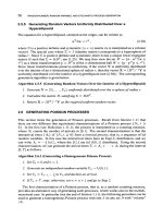
that at any point in time the realizations of
{
X,}
generated from the simulation run become
independent or constant. The situation is illustrated in Figure
4.3,
where the dashed curve
indicates the expectation of
Xt.
XI
A
transient regime
:
steady-state
regime
Figure
4.3
The state process
for
a dynamic simulation model.
The exact distributions (transient and steady-state) are usually available only for sim-
ple Markovian models such as the
M/M/1
queue. For non-Markovian models, usually
neither the distributions (transient and steady-state) nor even the associated moments are
available via analytical methods. For performance analysis of such models one must resort
to

simulation.
Note that for some stochastic models, only finite-horizon simulation is feasible, since
the steady-state regime either does not exist or the finite-horizon period is
so
long that the
steady-state analysis is computationally prohibitive (see, for example,
[9]).
4.3.1
Finite-Horizon Simulation
The statistical analysis for finite-horizon simulation models is basically the same as that for
static models. To illustrate the procedure, suppose that
{X,,
t
>
0)
is a continuous-time
process for which we wish to estimate the expected average value,
C(T,
m)
=
E
[T-’
iT
X,
dt]
,
(4.13)
as a function of the time horizon
T
and the initial state

XO
=
m.
(For a discrete-time
process
{Xt,
t
=
1,2,.
.
.}
the integral
so
X,
dt
is replaced by the sum
Ct=l
X,.)
As an
example, if
Xt
represents the number
of
customers in a queueing system at time
t,
then
C(T,
m)
is the average number of customers in the system during the time interval
[O,

TI,
given
Xo
=
m.
Assume now that
N
independent replications are performed, each starting at state
XO
=
m.
Then the point estimator and the
(1
-
a)
100% confidence interval for
C(T,
m)
can be
written, as in the static case (see (4.2) and (4.7))
,
as
T
T
N
F(T,
m)
=
N-’
c

y,
(qT,
m)
f
Z~-~/~SN-’/~
i=l
and
(4.14)
(4.15)
DYNAMIC
SIMULATION
MODELS
103
T
respectively, where
yt
=
T-'
so
Xti
dt,
Xti
is the observation at time
t
from the i-th
replication and
S2
is the sample variance of
{
yt}.

The algorithm for estimating the finite-
horizon performance,
e(T,
m),
is thus:
Algorithm
4.3.1
1.
Perform
N
independent replications
of
theprocess
{
Xt
,
t
<
T}, starting each repli-
cation from the initial state
XO
=
'm.
2.
Calculate the point estimator and the conjidence interval of
C(T,
rn)
from
(4.14)
and

(4.15),
respectively.
If, instead of the expected average number of customers, we want to estimate the expected
maximum
number of customers in the system during an interval
(0,
TI,
the only change
required is to replace
Y,
=
T-'
Xt,
dt
with
Y,
=
maxoGtGT
Xti.
In the same way, we
can estimate other performance measures for this system, such as the probability that the
maximum number of customers during
(0,
T]
exceeds some level
y
or
the expected average
period of time that the first
k

customers spend in the system.
4.3.2
Steady-State Simulation
Steady-state simulation concerns systems that exhibit some form of stationary or long-run
behavior. Loosely speaking, we view the system as having started in the infinite past,
so
that any information about initial conditions and starting times becomes irrelevant. The
more precise notion is that the system state is described by a
stationaly process;
see also
Section
1.12.
I
EXAMPLE
4.3
M/M/l
Queue
Consider the birth and death process
{
Xt
,
t
3
0)
describing the number of customers
in the
MIMI1
queue; see Example
1.13.
When the traffic intensity

e
=
X/p
is less
than
1,
this Markov jump process has a limiting distribution,
which is also its stationary distribution. When
XO
is distributed according to this
limiting distribution, the process
{Xt,
t
2
0)
is stationary: it behaves as if it has
been going on for an infinite period of time. In particular, the distribution of
Xt
does not depend on
t.
A
similar result holds for the Markov process
{
Z,,
n
=
1,2,.
.
.},
describing the number of customers in the system as seen by the n-th

arriving customer. It can be shown that under the condition
e
<
1
it has the
same
limiting distribution as
{Xt,
t
0).
Note that for the
MIMI1
queue the steady-
state expected performance measures are available analytically, while for the
GI/G/1
queue,
to
be discussed in Example
4.4,
one needs to resort to simulation.
Special care must be taken when making inferences concerning steady-state performance.
The reason is that the output data are typically correlated; consequently, the above statistical
analysis, based on independent observations, is no longer applicable.
In order to cancel the effects of the time dependence and the initial distribution, it is com-
mon practice to discard the data that are collected during the nonstationary
or
transient part
of the simulation. However, it is not always clear when the process will reach stationarity.
104
STATISTICAL ANALYSIS

OF
DISCRETE-EVENT SYSTEMS
If the process is regenerative, then the regenerative method, discussed in Section 4.3.2.2,
avoids this transience problem altogether.
From now on, we assume that
{X,}
is a stationary process. Suppose that we wish to
estimate the steady-state expected value
e
=
E[X,], for example, the expected steady-state
queue length, or the expected steady-state sojourn time of a customers in a queue. Then
!
can be estimated as either
T
or
t=l
T
e
=
T-~L
xt
dt
,
respectively, depending on whether
{
X,}
is a discrete-time or continuous-time process.
given bv
For concreteness, consider the discrete case. The variance of F(see Problem 1.15) is

Since
{Xt}
is stationary, we have Cov(X,,
X,)
=
E[X,Xt]
-
e2
=
R(t
-
s),
where
R
defines the
covariancefinction
of the stationary process. Note that
R(0)
=
Var(Xt).
As
a consequence, we can write (4.16) as
T-1
T
Var(6
=
R(0)
+
2
(I

-
$)
R(t)
.
t=l
(4.17)
Similarly,
if
{X,}
is a continuous-time process, the sum
in
(4.17) is replaced with the
corresponding integral (from
t
=
0
to
T),
while all other data remain the same. In many
applications
R(t)
decreases rapidly with
t,
so
that only the first few terms
in
the sum (4.17)
are relevant. These covariances, say
R(O),
R(1),

.
. .
,
R(K),
can be estimated via their
(unbiased) sample averages:
-
T-k
Thus, for large
T
the variance of ?can be estimated as
s2/T,
where
K
s2
=
2(0)
+
2
c
2(t)
t=l
To obtain confidence intervals, one again uses the central limit theorem, that is, the cdf of
n(F-
!)
converges to the cdf of the normal distribution with expectation
0
and variance
o2
=

limT,, T
Var(e) -the so-called
asymptotic variance
of
e.
Using
s2
as an estimator
for
c2,
we find that an approximate
(1
-
a)100%
confidence interval for
C
is given by
-
(4.18)
Below we consider two popular methods for estimating steady-state parameters: the
batch means
and
regenerative
methods.
DYNAMIC SIMULATION
MODELS
105
4.3.2.1
The Batch Means Method
The batch means method is most widely used by

simulation practitioners to estimate steady-state parameters from a single simulation run,
say of length
M.
The initial
K
observations, corresponding to the transient part of the run,
are deleted, and the remaining
M
-
K
observations are divided into
N
batches, each of
length
M-K
N
T=-
The deletion serves to eliminate or reduce the initial bias,
so
that the remaining observations
{
Xt
,
t
>
K}
are statistically more typical of the steady state.
Suppose we want to estimate the expected steady-state performance
C
=

E[Xt],
assuming
that the process
is
stationary for
t
>
K.
Assume for simplicity that
{X,}
is
a discrete-time
process. Let
Xti
denote the t-th observation from the i-th batch. The sample mean
of
the
i-th batch of length
T
is given by
.T
1
yI=&xLi:
i=1,
,
N
t=l
Therefore, the sample mean
tof
&?

is
The procedure is illustrated in Figure
4.4.
I I
I I
I
I
I
I
I
I
I’
I
I
I
I
I
I
I
I
I
I1
ot
I,
t
K
T
T
T
M

Figure
4.4
Illustration
of
the batch means procedure.
(4.19)
In order to ensure approximate independence between the batches, their size,
T,
should
be large enough. In order for the central limit theorem
to
hold approximately, the number of
batches,
N,
should typically be chosen in the range
20-30.
In such a case, an approximate
confidence interval fore is given by
(4.7),
where
S
is the sample standard deviation of the
{
Yi}.
In the case where the batch means do exhibit some dependence, we can apply formula
(4.18)
as an alternative to
(4.7).
106
STATISTICAL

ANALYSIS
OF
DISCRETE-EVENT
SYSTEMS
Next, we shall discuss briefly how to choose
K.
In general, this is a very difficult task,
since very few analytic results are available. The following queueing example provides
some hints on how
K
should be increased as the traffic intensity in the queue increases.
Let
{
Xt
,
t
2
0)
be the queue length process (not including the customer in service) in an
M/M/l
queue, and assume that we start the simulation at time zero with an empty queue.
It is shown in
[I,
21
that in order to be within
1
%
of the steady-state mean, the length of the
initial portion to be deleted,
K,

should be on the order
of
8/(p(1
-
e)*), where
l/p
is
the
expected service time. Thus, fore
=
0.5,
0.8,
0.9,
and
0.95,
K
equals
32,
200,
800,
and
3200 expected service times, respectively.
In general, one can use the following simple rule of thumb.
1. Define the following moving average
Ak
of length
T:
.
T+k
1

Ak
=
-
C
Xt
t=k+1
T
2. Calculate
A,+
for different values of
k,
say
k
=
0,
m,,
2m,.
.
.
,
rm,
. .
.,
where
7n
is
fixed, say
m
=
10.

3.
Find
r
such that
A,,
=z
A(,+l),,,
'
. .
zz
A(r+s)my
while
A(,-s)m
$
A(r-s+l)m
$
. . .
$
A,,,
where
r
2
s
and
s
=
5,
for example.
4.
Deliver

K
=
rm.
The batch means algorithm is as follows:
Algorithm
4.3.2
(Batch Means Method)
I.
Make a single simulation
run
of
length
M
anddelete
K
observations corresponding
to ajnite-horizon simulation.
2.
Divide the remaining
M
-
K
observations into
N
batches, each
of
length
A4
-
K

T=-
N'
3.
Calculate the point estimator and the conjdence interval for
l?
from
(4.19)
and
(4.7),
respectively.
EXAMPLE
4.4
GI/G/1
Queue
The
GI/G/l
queueing model is a generalization of the
M/M/l
model discussed in
Examples
1.13
and 4.3. The only differences are that
(1)
the interarrival times each
have a general cdf
F
and (2) the service times each have a general cdf
G.
Consider
the process

{Zn,
n
=
1,2,.
.
.}
describing the number of people in a
GI/G/l
queue
as seen by the n-th arriving customer. Figure 4.5 gives a realization of the batch
means procedure for estimating the steady-state queue length. In this example the
first
K
=
100
observations are thrown away, leaving
N
=
9
batches, each of size
T
=
100.
The batch means are indicated by thick lines.
DYNAMIC
SIMULATION
MODELS
107




I

.

0 0-




4

.,o

.I
. .
" ,.
-,.I
.I.


-4
."#

"-


200
400
600

800
1000
Figure
4.5
The batch means
for
the process
{Zn,
n
=
1,2,.
.
.}
Remark
4.3.1
(Replication-Deletion Method)
In the replication-deletion method
N
in-
dependent runs are carried out, rather than a single simulation run as in the batch means
method. From each replication, one deletes
K
initial observations corresponding to the
finite-horizon simulation and then calculates the point estimator and the confidence interval
for
C
via (4.19) and (4.7), respectively, exactly as in the batch means approach. Note that the
confidence interval obtained with the replication-deletion method is unbiased, whereas the
one obtained by the batch means method is slightly biased. However, the former requires
deletion from

each
replication, as compared to
a
single
deletion in the latter. For this rea-
son, the former is not as popular as the latter.
For
more details on the replication-deletion
method see [9].
4.3.2.2
The Regenerative Method
A stochastic process
{
X,}
is called
regenerative
if there exist random time points
To
<
Tl
<
T2
<
.
.
.
such that at each such time point
the process restarts probabilistically. More precisely, the process
{X,}
can be split into iid

replicas during intervals, called
cycles,
of
lengths
~i
=
T,
-
Ti-1,
i
=
1,2,
.
.

W
EXAMPLE
4.5
Markov Chain
The standard example of a regenerative process is a Markov chain. Assume that the
chain starts from state
i.
Let
TO
<
2'1
<
2'2
<
. .

.
denote the times that it visits state
j.
Note that at each random time
T,,
the Markov chain starts afresh, independently of
the past. We say that the Markov process
regenerates
itself. For example, consider a
two-state Markov chain with transition matrix
i
m
_.^
\
Yll
Yll
p=
(
P2l
P22
)
(4.20)
Assume that all four transition probabilities
p,,
are strictly positive and that, starting
from state
1
=
1,
we obtain the following sample trajectory:

(50,21,22,.
'.
,210)
=
(1,2,2,2,1,2,1,1,2,2,1)
'
It is readily seen that the transition probabilities corresponding to the above sample
trajectory are
P121
P22r
P22r
P21,
P12r
P21,
Pll, Pl2,
P221
P21
'
108
STATISTICAL
ANALYSIS
OF
DISCRETE-EVENT
SYSTEMS
Taking
j
=
1
as the regenerative state, the trajectory contains four cycles with the
following transitions:

1-+2-+2-+2-1; 1-2-1; 1-1; 1-+2-+2+1,
and the corresponding cycle lengths are
71
=
4,
72
=
2,
73
=
1,
74
=
3.
W
EXAMPLE 4.6
GI/G/1
Queue (Continued)
Another classic example of a regenerative process is the process
{
Xt,
t
2
0)
de-
scribing the number
of
customers in the
GIIGI1
system, where the regeneration

times
TO
<
TI
<
T2
<
.
.
.
correspond to customers arriving at an empty system
(see also Example
4.4,
where a related discrete-time process is considered). Observe
that at each such time
Ti
the process starts afresh, independently
of
the past; in other
words, the process regenerates itself. Figure
4.6
illustrates a typical sample path
of
the process
{Xt,
t
2
0).
Note that here
TO

=
0,
that is, at time
0
a
customer arrives
at an empty system.
f
* ,







D
Cycle
1
Cycle
2
Cycle
3
Figure
4.6
GIfGf1
queue.
A
sample path
of

the process
{Xt,
t
2
0).
describing the number of customers
in
a
EXAMPLE 4.7
(3,
s)
Policy
Inventory Model
Consider a continuous-review, single-commodity inventory model supplying external
demands and receiving stock from a production facility. When demand occurs, it
is either filled or back-ordered (to be satisfied by delayed deliveries). At time
t,
the
net inventory
(on-hand inventory minus back orders) is
Nt,
and the
inventory
position
(net inventory plus on-order inventory)
is
Xt.
The control policy is an
(s,
S)

policy that operates on the inventory position. Specifically, at any time
t
when a
demand
D
is received that would reduce the inventory position to less than
s
(that is,
Xt-
-
D
<
s,
where
Xt-
denotes the inventory position just before
t),
an order
of
size
S
-
(Xt-
-
D)
is placed, which brings the inventory position immediately back
to
S.
Otherwise, no action is taken. The order arrives
T

time units after it is placed
(T
is called the
lead
time). Clearly,
Xt
=
Nt
if
T
=
0.
Both inventory processes are
illustrated in Figure
4.7.
The dots in the graph of the inventory position (below the
s-line) represent what the inventory position would have been
if
no order was placed.
DYNAMIC
SIMULATION
MODELS
109
-
Figure
4.7
Sample paths
for
the
two

inventory
processes.
Let
D,
and
A,
be the size of the i-th demand and the length of the i-th inter-
demand time, respectively. We assume that both
{ D,}
and
{
A,}
are iid sequences,
with common cdfs Fand
G,
respectively. In addition, the sequences areassumed to be
independent of each other. Under the back-order policy and the above assumptions,
both the inventory position process
{X,}
and the net inventory process
{Nt}
are
regenerative.
In particular, each process regenerates when it is raised to
S.
For
example, each time an order is placed, the inventory position process regenerates. It
is readily seen that the sample path of
{
X,}

in Figure
4.7
contains three regenerative
cycles, while the sample path of
{
Nt
}
contains only two, which occur after the second
and third lead times. Note that during these times no order has been placed.
The main strengths of the concept of regenerative processes are that the existence of
limiting distributions is guaranteed under very mild conditions and the behavior
of
the
limiting distribution depends only on the behavior of the process during a typical cycle.
Let
{
X,}
be a regenerative process with regeneration times
To,T~,
Tz,
. .
Let
T,
=
Ti
-
T,-
1,
z
=

1,2,
.
. .
be the cycle lengths. Depending on whether
{
X,}
is a discrete-time
or continuous-time process, define, for some real-valued function
H,
Ti
-
1
Ri
=
-1-
H(X,)
(4.21)
11
0
STATISTICAL
ANALYSIS
OF
DISCRETE-EVENT
SYSTEMS
or
(4.22)
respectively, for
i
=
1,2,.

.

We assume for simplicity that
To
=
0.
We also assume that
in the discrete case the cycle lengths are not always a multiple of some integer greater than
1.
We can view Ri as the reward (or, alternatively, the cost) accrued during the i-th cycle.
Let
=
2'1
be the length of the first regeneration cycle and let
R
=
R1
be the first reward.
The following properties of regenerative processes will be needed later on; see, for
example,
[3].
(a) If
{Xt}
is regenerative, then the process
{
H(Xt)}
is regenerative as well.
(b) If
E[T]
<

m,
then, under mild conditions, the process
{X,}
has a limiting (or steady-
state) distribution, in the sense that there exists a random variable
X,
such that
Iim
P(Xt
<
x)
=
P(X
<
Z)
t-cc
In the discrete case, no extra condition is required. In the continuous case a sufficient
condition is that the sample paths of the process are right-continuous and that the
cycle length distribution is
non-lattice-
that is, the distribution does not concentrate
all its probability mass at points
nb,
n
E
N,
for some
b
>
0.

(c) If the conditions in (b) hold, the steady-state expected value,
L
=
E[H(X)],
is given
bv
(4.23)
(d) (Ri,
~i),
i
=
1,2,
. . .
,
is a sequence of iid random vectors.
Note that property (a) states that the behavior patterns of the system
(or
any measurable
function thereof) during distinct cycles are statistically iid, while property (d) asserts that
rewards and cycle lengths are jointly iid for distinct cycles. Formula
(4.23)
is fundamental
to regenerative simulation. For typical non-Markovian queueing models, the quantity
e
(the steady-state expected performance) is unknown and must be evaluated via regenerative
simulation.
To
obtain a point estimate of
l!,
one generates

N
regenerative cycles, calculates the iid
sequence of two-dimensional random vectors
(Ri,
~i),
i
=
1,
. . .
,
N,
and finally estimates
f?
by the
ratio
estimator
-R
e=
-
,
7
(4.24)
h
where
is,
E[a
#
L.
However,
as

N
-+
00.
This follows directly from the fact that, by the law of large numbers,
converge with probability
1
to
E[R]
and
lE[7],
respectively.
=
N-'
c,"=,
Ri and
?
=
N-'
c,"=,
~i.
Note that the estimator
e
is biased, that
is
strongly consistent,
that is, it converges to
e
with probability
1
and

?
The
advantages
of the regenerative simulation method are:
(a) No deletion of transient data
is
necessary.
(b) It is asymptotically exact.
(b) It is easy to understand and implement.
DYNAMIC SIMULATION MODELS
11
1
The disadvantages of the regenerative simulation method are:
(a) For many practical cases, the output process,
{
Xt},
is either nonregenerative or its
regeneration points are difficult to identify. Moreover, in complex systems
(for
ex-
ample, large queueing networks), checking for the occurrence of regeneration points
could be computationally expensive.
(b) The estimator Fis biased.
(c) The regenerative cycles may be very long.
Next, we shall establish a confidence interval fore. Let
Zi
=
R,
-
It is re_adily seen

that the
2,
are iid random variables, like the random vectors
(Ri,
~i).
Letting
R
and
7
be
defined as before, the central limit theorem ensures that
~1/2
(5
-
e?)
"12
(F-
e)
-
-
(T
u/7
converges
in
distribution to the standard normal distribution as
N
+
00,
where
o2

=
Var(2)
=
Var(R)
-
2eCov(R,
7)
+
C2
Var(.r)
.
(4.25)
Therefore, a
(1
-
ct)lOO%
confidence interval fore
=
E[R]/E(T]
is
(F*
H)
,
(4.26)
(4.27)
is the estimator of
(T'
based
on
replacing the unknown quantities

in
(4.25) with their unbiased
estimators. That is.
.N
.N
X(Ti
-
?)2
1 1
s22
=
-
N-1
s11
=
-
C(Ri
-
Z)',
i=l
i=l
N-1
and
Note that (4.26) differs from the standard confidence interval, say (4.7), by having an
additional term
?.
The algorithm for estimating the
(1
-
a)

100%
confidence interval for
e
is as follows:
Algorithm
4.3.3
(Regenerative Simulation Method)
I.
Simulate
N
regenerative cycles
of
the process
{
X,}
.
2.
Compute the sequence
{
(Ri,
Ti),
z
=
1,
. .
.
,
N}.
3.
Calculate the point estimator

Fond
the conjidence interval
of
C
from
(4.24)
and
(4.26),
respectively
1
12
STATISTICAL ANALYSIS
OF
DISCRETE-EVENT SYSTEMS
Note that if one uses two independent simulations of length
N,
one for estimating lE[R] and
the other for estimating
IE[r],
then clearly
S2
=
5’11
+
e
2S22,
since Cov(R,
r)
=
0.

Remark
4.3.2
If the reward in each cycle is of the form
(4.21)
or
(4.22),
then
e
=
E[H(X)]
can be viewed as both the expected steady-state performance and the long-run average
performance. This last interpretation is valid even if the reward in each cycle is not of the
form
(4.21)-(4.22)
as long as the
{
(ri,
R,)} are iid. In that case,
(4.28)
where
Nt
is the number of regenerations in
[0,
t].
rn
EXAMPLE
4.8
Markov Chain: Example
4.5
(Continued)

Consider again the two-state Markov chain with the transition matrix
Pll
P12
=
(
P21 P22
)
Assume, as in Example
4.5,
that starting from
1
we obtain the following sample
trajectory:
(~0~~1,
ZZ,
. . .
,210)
=
(1,2,2,2,
I,
2,1,
I,
2,2,
I),
which has four cy-
cles with lengths
r1
=
4,
72

=
2,
73
=
1,
74
=
3
and corresponding transitions
(~12,~22,~22,~21), (~12~~21)~
PI^),
(~12,~22,~21).
In addition, assume that each
transition from
i
to
j
incurs a cost (or, alternatively, a reward)
cij
and that the related
cost matrix is
c
=
(Cij)
=
(
;;;
;;;
)
=

(
;
;
)
Note that the cost in each cycle
is
not of the form (4.21) (however, see Problem
4.14)
but is given as
We illustrate the estimation procedure for the long-run average cost
e.
First, observe
that
R1
=
1
+
3
+
3
+
2
=
9,
R2
=
3,
R3
=
0,

a_”d
R4
=
6.
It follows that
5
=
4.5.
Since
?
=
2.5,
the point estimate of
e
is
e
=
1.80.
Moreover,
Sll
=
15,S22
=
513,
S12
=
5,
and
S2
=

2.4.
This gives a
95%
confidence interval fore
of
(1.20,2.40).
rn
EXAMPLE
4.9
Example
4.6
(Continued)
Consider the sample path in Figure
4.6
of the process
{
Xt,
t
2
0)
describing the
number of customers in the
GZ/G/1
system. The corresponding sample path data
are given in Table
4.2.
THE BOOTSTRAP METHOD
11
3
Table

4.2
Sample path data for the
GI/G/l
queueing process.
t
E
interval
Xt
t
E
interval
Xt
t
E
interval
Xt
[O.OO,
0.80)
1
[3.91,4.84)
1
[6.72,7.92)
1
[0.80,1.93)
2
[4.84,6.72)
0
[7.92,9.07)
2
[1.93,2.56)

1
[9.07,10.15)
1
[2.56,3.91)
0
[10.15,11.61)
0
Cycle
1
Cycle
2
Cycle
3
Notice that the figure and table reveal three complete cycles with the follow-
ing pairs:
(R1,~1)
=
(3.69,3.91),
(R2,5)
=
(0.93,2.81),
and
(R3,73)
=
(4.58,4.89).
The resultant statistics are (rounded)
e
=
0.79,
,911

=
3.62,
S22
=
1.08,
S12
=
1.92,
S2
=
1.26
and the
95%
confidence interval is
(0.79
f
0.32).
A
EXAMPLE
4.10
Example
4.7
(Continued)
Let
{Xt,
t
2
0)
be the inventory position process described in Example 4.7. Table
4.3

presents the data corresponding to the sample path in Figure
4.7
for a case where
s
=
10,
S
=
40,
and
T
=
1.
Table
4.3
boxes
indicate the regeneration times.
The data for the inventory position process,
{Xt},
with
s
=
10
and
S
=
40.
The
t
Xt

t
Xt
t
Xl
40.00 40.00 40.00
1.79 32.34 6.41 33.91 11.29 32.20
3.60 22.67 6.45 23.93 11.38 24.97
5.56 20.88 6.74 19.53 12.05 18.84
5.62 11.90 8.25 13.32 13.88 13.00
9.31 10.51
114.71)
40.00
Based on the data in Table
4.3,
we illustrate the derivation of the point esti-
mator and the
95%
confidence interval for the steady-state quantity
k!
=
P(X
<
30)
=
!E[I~x<30)],
that is, the probability that the inventory position is less
than
30.
Table
4.3

reveals three complete cycles with the following pairs:
(RI,~)
=
(2.39,5.99),
(Rz,T~)
=
(3.22,3.68),
and
(R3,~3)
=
(3.33,5.04),
A
where
Ri
=
J:-l
Itxt<30)
dt.
The resulting statistics are (rounded)
k!
=
0.61,
S11
=
0.26,
522
=
1.35,
Sl2
=

-0.44,
and
S2
=
1.30,
which gives a
95%
confidence interval
(0.61
f
0.26).
4.4
THE BOOTSTRAP METHOD
Suppose we estimate a number
e
via some estimator
H
=
H(X),
where
X
=
(XI,
. . .
,
Xn),
and the
{Xi}
form a random sample from some unknown distribution
F.

It
114
STATISTICAL
ANALYSIS
OF
DISCRETE-EVENT
SYSTEMS
is assumed that
H
does not depend on the order of the
{Xi}.
To
assess the quality (for ex-
ample, accuracy) of the estimator
H,
one could draw independent replications
X1
. .
XN
of
X
and find sample estimates for quantities such as the variance of the estimator
Var(H)
=
E[H~]
-
(IE[II])',
the
bias
of the estimator

Bias
=
E[H]
-
P,
and the expected quadratic error, or
mean square error
(MSE)
MSE
=
E
[(H
-
1)2]
.
However, it may be too time-consuming, or simply not feasible, to obtain such replications.
An alternative is to
resample
the original data. Specifically, given an outcome
(51,
. .
.
,
2,)
of
X,
we draw a random sample
Xi,.
. .
X;

not from
F
but from an approximation
to
this
distribution. The best estimate that we have about
F
on the grounds of
{xi}
is the
empirical
distribution,
F,,,
which assigns probability mass
l/n
to each point
zi,
i
=
1,.
.
.
n.
In
the
one-dimensional case, the cdf of the empirical distribution
is
thus given by
Drawing from this distribution is trivial: for each
j,

draw
U
-
U[O,
11,
let
J
=
LU
n]
+
1,
and return
X;
=
x
J.
Note that if the
{xi}
are all different, vector
X*
=
(XT,
.
. .
,
X;)
can take
nn
different values.

The rationale behind the resampling idea is that the empirical distribution
F,
is close to
the actual distribution
F
and gets closer as
n
gets larger. Hence, any quantities depending
on
F,
such as
lE~[h(H)l,
where
h
is a function, can be approximated by
EF,
[h(H)].
The
latter is usually still difficult to evaluate, but it can be simply estimated via Monte Carlo
simulation as
where
H;,
.
.
.
,
Hi
are independent copies of
H'
=

H(X*).
This seemingly self-referent
procedure is called
bootstrapping
-
alluding to Baron von Munchhausen, who pulled
himself out
of
a swamp by his own bootstraps. As an example, the bootstrap estimate of
the expectation of
H
is
which is simply the sample mean of
{lit}.
Similarly, the bootstrap estimate for Var(
H)
is
the sample variance
B
C(H;
-
z*y.
1
B-1
Var(f1)
=
-
(4.29)
i=l
Perhaps of more interest are the bootstrap estimators for the bias and MSE, respectively

H
-Hand
-*
-B
1
-
C(H,'
-
H)2
.
i=l
B
PROBLEMS
115
Note that for these estimators the unknown quantity
C
is replaced with the original estimator
H.
Confidence intervals can be constructed
in
the same fashion. We discuss two variants:
the
normal
method and the
percentile
method. In the normal method, a (1
-
&)loo%
confidence interval for
e

is given by
(H
f
&r/2S*)
>
where
S’
is the bootstrap estimate of the standard deviation of
H,
that is, the square root of
(4.29). In the percentile method, the upper and lower bounds of the
(1
-a)
100%
confidence
interval fore are given by the
1
-
a/2 and a/2 quantiles of
H,
which in turn are estimated
via the corresponding sample quantiles of the bootstrap sample
{
Hf
}.
PROBLEMS
4.1
We wish to estimate
C
=

f2
e-x2/2
dz
=
s
H(z)f(z)
dz
via Monte Carlo simu-
lation using two different approaches: (a) defining
H(z)
=
4
ecX2/’ and
f
the pdf of the
U[-2,2] distribution and (b) defining
H(z)
=
&
I{-2,,,2)
and
f
the pdf of the
N(0,l)
distribution.
a)
For both cases, estimate
C
via the estimator Fin (4.2). Use a sample size of
b)

For both cases, estimate the relative error oft using
N
=
100.
c)
Give a
95%
confidence interval for
C
for both cases, using
N
=
100.
d)
From
b),
assess how large
N
should be such that the relative width of the con-
fidence interval is less than 0.001, and carry out the simulation with this
N.
Compare the result with the true value of
e.
4.2
Prove that the structure function of the bridge system in Figure 4.1 is given by (4.3).
4.3
Consider the bridge system in Figure 4.1. Suppose all link reliabilities are
p.
Show
that the reliability of the system is p2(2

+
2
p
-
5
p2
+
2
p3).
4.4
Estimate the reliability of the bridge system in Figure 4.1 via (4.2) if the link reli-
abilities are
(PI,.
.
.
,
p5)
=
(0.7,
0.6,
0.5,
0.4,
0.3).
Choose a sample size such that the
estimate has a relative error of about
0.01.
4.5
N
=
100.

Consider the following sample performance:
Assume that the random variables X,,
1:
=
1,.
.
.
,5
are iid with common distribution
(a)
Gamma(Xt,
PE),
where
A,
=
i
and
pL
=
i.
(b)
Ber(pi),
where
pi
=
1/22,
Run a computer simulation with
N
=
1000

replications, and find point estimates and
95%
confidence intervals for
E
=
IE[H(X)].
4.6
Consider the precedence ordering of activities in Table 4.4. Suppose that durations
of the activities (when actually started) are independent of each other, and all have expo-
nential distributions with parameters
1
.l, 2.3, 1.5, 2.9,
0.7,
and
1.5,
for activities
1,
.
. .
,6,
respectively.
1
16
STATISTICAL ANALYSIS
OF
DISCRETE-EVENT SYSTEMS
Table
4.4
Precedence ordering
of

activities.
Activity
1
2
3
4
5
6
Predecessor(s)
-
-
1
2,3 2,3
5
n
Figure
4.8
The
PERT
network corresponding to Table
4.4.
a)
Verify that the corresponding PERT graph is given by Figure
4.8.
b)
Identify the four possible paths from start to finish.
c)
Estimate the expected length of the critical path in
(4.5)
with a relative error of

4.7
Let
{
Xt,
t
=
0,
1,2,
.
.
.}
be a random walk on the positive integers; see Example 1.1 1.
Suppose that
p
=
0.55 and
q
=
0.45. Let
Xo
=
0.
Let
Y
be the maximum position reached
after 100 transitions. Estimate the probability that
Y
2
15
and give a 95% confidence

interval for this probability based on 1000 replications of
Y.
4.8
Consider the
MIMI1
queue. Let
Xt
be the number of customers in the system at
time
t
>
0.
Run a computer simulation of the process
{
Xt,
t
>
0)
with
X
=
1
and
p
=
2,
starting with an empty system. Let
X
denote the steady-state number of people in the
system. Find point estimates and confidence intervals for

C
=
IE[X],
using the batch means
and regenerative methods as follows:
a)
For the batch means method run the system for a simulation time of
10,000,
discard the observations in the interval [0,100], and use
N
=
30
batches.
b)
For the regenerative method, run the system for the same amount of simulation
time
(10,000)
and take as regeneration points the times where an amving customer
finds the system empty.
c)
For both methods, find the requisite simulation time that ensures a relative width
of the confidence interval not exceeding
5%.
4.9
Let
2,
be the number of customers in an
MIMI1
queueing system, as seen by the
n,-th arriving customer,

ri
=
1,2,
. .
Suppose that the service rate is
p
=
1
and the arrival
rate is
X
=
0.6.
Let
2
be the steady-state queue length (as seen by an arriving customer
far away in the future). Note that
2,
=
XT,
with
Xt
as in Problem
4.8,
and
T,
is the
arrival epoch of the n-th customer. Here,
“T,
-”

denotes the time just before
T,.
less than
5%.
a)
Verify that
C
=
E[Z]
=
1.5.
b)
Explain how to generate
{Z,,,
n
=
1,2,
.
.
.}
using a random walk on the positive
integers, as in Problem
4.7.
c)
Find the point estimate of
e
and a 95% confidence interval for
e
using the batch
means method. Use a sample size of

lo4
customers and
N
=
30
batches, throwing
away the first
K
=
100 observations.
PROBLEMS
117
d)
Do the same as in c) using the regenerative method instead.
e)
Assess the minimum length of the simulation run in order to obtain a
95%
confi-
dence interval with an absolute width
wa
not exceeding
5%.
f)
Repeat c), d), and e) with
e
=
0.8
and discuss c). d), and e)
as
e

-+
1.
4.10
Table 4.5 displays a realization of a Markov chain,
{Xt,
t
=
0,1,2,
.
.
.},
with state
space
{0,1,2,3}
starting at
0.
Let
X
be distributed according to the limiting distribution
of this chain (assuming it has one).
Table
4.5
A
realization
of
the
Markov
chain.
Find the point estimator,
and the

95%
confidence interval for
C
=
E[X]
using the
regenerative method.
4.11
Let
W,
be the
waiting time
of the n-th customer in a
GI/G/l
queue, that
is,
the
total time the customer spends waiting in the queue (thus excluding the service time).
The waiting time process
{
W,,
n
=
1,2,
.
.
.}
follows the following well-known
Lzndley
equation:

(4.30)
where
A,+1
is the interval between the n-th and
(n
+
1)-st arrivals,
S,
is the service time
of the n-th customer, and
W1
=
0
(the first customer does not have to wait and is served
immediately).
Wn+l
=
max{Wn
+
S,
-
A,+1,
0},
n
=
1,2,.
. .,
a)
Explain why the Lindley equation holds.
b)

Find the point estimate and the
95%
confidence interval for the expected waiting
time for the 4-th customer in an
M/M/l
queue with
e
=
0.5,
(A
=
I),
starting
with an empty system. Use
N
=
5000
replications.
c)
Find point estimates and confidence intervals for the expected average waiting
time for customers
21,.
.
.
,70
in the same system as in b). Use
N
=
5000
replications. Hint: the point estimate and confidence interval required are for the

following parameter:
4.12
Run a computer simulation of 1000regenerativecycles of the
(s,
S)
policy inventory
model (see Example 4.7), where demands arrive according to a Poisson process with rate
2
(that is,
A
-
Exp(2))
and the size of each demand follows a Poisson distribution with mean
2
(that is,
D
-
Poi(2)).
Take
s
=
1,
S
=
6,
lead time
T
=
2,
and initial value

XO
=
4.
Find point estimates and confidence intervals for the quantity
e
=
P(2
<
X
<
4), where
X
is the steady-state inventory position.
4.13
Simulate the Markov chain
{X,}
in Example 4.8, using
pll
=
1/3
and
p22
=
3/4
for 1000 regeneration cycles. Obtain a confidence interval for the long-run average cost.
4.14
Consider Example 4.8 again, with
pll
=
1/3

and
p22
=
3/4.
Define
Y,
=
(XI,
X,+1)
and
H(Y,)
=
CX,,X,+,.
i
=
0,1,.
.

Show that
{Yt}
is a regenerative pro-
I
I8
STATISTICAL ANALYSIS
OF
DISCRETE-EVENT SYSTEMS
cess. Find the corresponding limitingkteady-state distribution and calculate
C
=
lE[H(

Y)],
where
Y
is distributed according to this limiting distribution. Check if
C
is
contained in the
confidence interval obtained in Problem 4.13.
4.15
Consider the tandem queue of Section 3.3.1. Let
Xt
and
Yt
denote the number
of
customers in the first and second queues at time
t,
including those who are possibly being
served.
Is
{
(Xt,
x),
t
2
0)
a regenerative process? If
so,
specify the regeneration times.
4.16

Consider the machine repair problem in Problem
3.5,
with three machines and two
repair facilities. Each repair facility can take only one failed machine. Suppose that the
lifetimes are
Exp(l/lO)
distributed and the repair times are
U(O,8)
distributed. Let
C
be
the limiting probability that all machines are out of order.
a)
Estimate
C
via the regenerativeestimator Fin (4.24) using
100
regeneration cycles.
Compute the
95%
confidence interval (4.27).
b)
Estimate the bias and MSE
of
Fusing the bootstrap method with a sample size of
B
=
300.
(Hint: theoriginaldataarex
=

(XI,.
. .
,
X~OO), wherexi
=
(Ri,
~i),
i
=
1,.
. .
,
100.
Resample from these data using the empirical distribution.)
c)
Compute
95%
bootstrap confidence intervals fort using the normal and percentile
methods with
B
=
1000
bootstrap samples.
Further Reading
The regenerative method in a simulation context was introduced and developed by Crane
and Iglehart [4,
51.
A
more complete treatment of regenerative processes is given in
[3].

Fishman
[7]
treats the statistical analysis of simulation data in great detail.
Gross
and Harris
[8]
is
a
classical reference on queueing systems. Efron and Tibshirani
[6]
gives the defining
introduction to the bootstrap method.
REFERENCES
1.
J.
Abate and
W.
Whitt. Transient behavior
of
regulated Brownian motion,
I:
starting at the origin.
2.
J.
Abate and W. Whitt. Transient behavior
of
regulated Brownian motion,
11:
non-zero initial
3.

S.
Asmussen.
AppliedProbability and
Queues.
John Wiley
&
Sons, New
York,
1987.
4. M.
A.
Crane
and
D.
L.
Iglehart. Simulating stable stochastic systems,
I:
general multiserver
5. M. A. Crane and
D.
L.
Iglehart. Simulating stable stochastic systems, 11: Markov chains.
Journal
6.
B.
Efron and
R.
Tibshirani.
An
Introduction to the Bootstrap.

Chapman
&
Hall, New
York,
7.
G.
S.
Fishman.
Monte Carlo: Concepts, Algorithms and Applications.
Springer-Verlag, New
8.
D.
Gross
and C. M. Hams.
Fundamentals
of Queueing
Theory.
John Wiley
&
Sons, New
York,
9. A. M. Law and
W.
D.
Kelton.
Simulation Modeling anddnalysis.
McGraw-Hill, New
York,
3rd
Advances

in
Applied Probability,
19560-598, 1987.
conditions.
Advances
in
Applied Probability,
19:599-631, 1987.
queues.
Journal
of
the ACM,
21:103-113, 1974.
of
the
ACM,
21:114-123, 1974.
1994.
York,
1996.
2nd edition, 1985.
edition, 2000.
CHAPTER
5
CONTROLLING THE VARIANCE
5.1
INTRODUCTION
This chapter treats basic theoretical and practical aspects of
variance reduction
techniques.

Variance reduction can be viewed as a means of utilizing known information about the
model in order to obtain more accurate estimators of its performance. Generally, the more
we know about the system, the more effective is the variance reduction. One way of
gaining this information is through a pilot simulation run of the model. Results from
this first-stage simulation can then be used to formulate variance reduction techniques that
will subsequently improve the accuracy of the estimators in the second simulation stage.
The main and most effective techniques for variance reduction are
importance sampling
and
conditional Monte Carlo.
Other well-known techniques that can provide moderate
variance reduction include the use of common and antithetic variables, control variables,
and stratification.
The rest of this chapter is organized as follows. We start, in Sections
5.2-5.5,
with
common and antithetic variables, control variables, conditional Monte Carlo, and stratified
sampling. However, most of our attention, from Section
5.6
on, is focused on
impor-
tance sampling
and
likelihood ratio
techniques. Using importance sampling, one can often
achieve substantial (sometimes dramatic) variance reduction, in particular when estimating
rare-event probabilities. In Section
5.6
we present two alternative importance sampling-
based techniques, called the

variance minimization
and
cross-entropy
methods. Section
5.7
discusses how importance sampling can be carried out
sequentially/dynamically.
Section
5.8
presents a simple, convenient, and unifying way of constructing efficient importance
Simulation
andthe
Monte
Carlo
Method,
Second
Edition.
By R.Y. Rubinstein
and
D.
P.
Kroese
119
Copyright
@
2007
John
Wiley
&
Sons,

Inc.
120
CONTROLLING
THE
VARIANCE
sampling estimators: the so-called
transform likelihood ratio
(TLR) method. Finally, in
Section
5.9
we present the
screening
method for variance reduction, which can also be seen
as a dimension-reduction technique. The aim of this method is to identify (screen out) the
most important (bottleneck) parameters of the simulated system to be used in an importance
sampling estimation procedure.
5.2
COMMON AND ANTITHETIC RANDOM VARIABLES
To
motivate the use of common and antithetic random variables in simulation, consider the
following simple example. Let
X
and Y be random variables with known cdfs,
F
and
G,
respectively. Suppose we want to estimate
e
=
E[X

-
Y]
via simulation. The simplest
unbiased estimator for
e
is
X
-
Y.
Suppose we draw
X
and
Y
via the IT method:
x
=
F-'(Ul)
,
U'
N
U(0,l)
,
U2
-
U(O,
1)
.
Y
=
G-'(U2)

,
The important point to notice is that
X
and
Y
(or
U1
and
lJ2)
need not be independent.
In
fact, since
Var(X
-
Y)
=
Var(X)
+
Var(Y)
-
2Cov(X,
Y)
(5.2)
and since the marginal cdfs of
X
and
Y
have been prescribed, it follows that the variance of
X
-

Y is minimized by maximizing the covariance in
(5.2).
We say that
common random
variables
are used in
(5.1)
if U2
=
Ul
and that
antithetic random variables
are used if
U2
=
1
-
U1.
Since both
F-'
and
G-'
are nondecreasing functions, it is readily seen that
using common random variables implies
Cov (F-'(U),
G-'(U))
>
0
for
U

-
U(0,l).
Consequently, variance reduction
is
achieved, in the sense that the
estimator
F-'(U)
-
G-'(U) has a smaller variance than the
crude Monte Carlo
(CMC)
estimator
X
-
Y, where
X
and Y are independent, with cdfs
F
and
G,
respectively. In fact,
it is well known (see, for example,
[35])
that using common random variables maximizes
the covariance between
X
and Y,
so
that Var(X
-

Y) is
minimized.
Similarly, Var(X
+
Y)
is minimized when antithetic random variables are used.
Now considerminimal variance estimation of
E[Hl(X)
-
H2(Y)], where
X
and Y are
unidimensional variables with known marginal cdfs,
F
and G, respectively, and
HI
and
Ef2 are real-valued monotone functions. Mathematically, the problem can be formulated as
follows:
Within
the
set
of
all
two-dimensional
joint
cdfs
of
(X,
Y).

find
a
joint cdf,
F',
that
minimizes Var(HI(X)
-
H2(Y)),
subject
to
X
and
Y
having
the
prescribed
cdfs
F
and
G,
respectively.
This problem has been solved by Gal, Rubinstein, and Ziv
[
111,
who proved that if
HI
and
H2
are monotonic in the
same

direction, then the use of common random variables leads
to optimal variance reduction, that is,
minVar(Hl(X)
-
H2(Y))
=
Var (Hl[F-'(U)]
-
Hz[G-'(U)])
.
(5.3)
The proof of
(5.3)
uses the fact that if
H(u)
is
a monotonic function, then
H(F-'(U))
is
monotonic as well, since
F-'(u)
is. By symmetry, if
H1
and
H2
are monotonic in
opposite
F'
COMMON AND ANTITHETIC RANDOM VARIABLES
121

directions, then the use of antithetic random variables (that is,
U2
=
1
-
Ul)
yields optimal
variance reduction.
This result can be further generalized by considering minimal variance estimation of
IE[ffl(X)
-
ff2(Y)I
I
(5.4)
where
X
=
(XI,.
. .
,
X,)
and
Y
=
(Y1,

.
,
Yn)
are random vectors with

X,
N
F,
and
Y,
N
G,,
i
=
1,.
.
.
,
n,
and the functions
H1
and
H2
are real-valued and monotone in
each component of
X
and
Y.
If the pairs
{
(X,,
Y,)}
are independent and
H1
and

H2
are
monotonic in the same direction (for each component), then the use of common random
variables again leads
to
minimal variance. That is, we take
X,
=
F,-'(U,)
and
Y,
=
GL1(U,),
i
=
1,.
.
.
,n,
where
U1,.
. .
,
U,
are independent
U(0,
1)-distributed random
variables, or, symbolically,
x
=

F-yu),
Y
=
G-'(U)
.
(5.5)
Similarly, if
H1
and
H2
are monotonic in opposite directions, then using antithetic random
variables is optimal. Finally, if
H1
and
H2
are monotonically increasing with respect
to
some components and monotonically decreasing with respect
to
others, then minimal
variance is obtained by using the appropriatecombination of common and antithetic random
variables.
We now describe one of the main applications of antithetic random variables. Suppose
one wants
to
estimate
e
=
E[H(X)I
>

where
X
-
F
is a random vector with independent components and the sample performance
function,
EZ(x),
is monotonic in each component of
x.
An example of such
a
function is
given below.
EXAMPLE
5.1
Stochastic Shortest Path
Consider the undirected graph in Figure
5.1,
depicting a so-called
bridge
network.
Figure
5.1
Determine
the
shortest path
from
A
to
B

in
a
bridge
network.
Suppose we wish
to
estimate the expected length
e
of the shortest path between
nodes (vertices)
A
and
B,
where the lengths of the links (edges) are random variables
XI,.
. .
,
X5.
We have
e
=
E[H(X)],
where
122
CONTROLLING
THE
VARIANCE
Note that
H(x)
is nondecreasing in each component of the vector

x.
edge lengths
{Xi}
can be written as
Similarly, the length
of
the shortest path H(X) in an arbitrary network with random
where
9j
is the j-th complete path from the source to the sink of the network
and
p
is the number of complete paths in the network. The sample performance is
nondecreasing in each
of
the components.
An unbiased estimator
of
d
=
E[H(X)] is the CMC estimator, given by
.N
where XI,.
.
.
,
XN
is an iid sample from the (multidimensional) cdf
F.
An alternative

unbiased estimator
of
C,
for
N
even, is
Nl2
1
=
c
{H(Xk)
+
H(Xt))},
k=
1
(5.9)
where
xk
=
F-l(uk)
and
xt)
=
F-l(l
-
Uk), using notation similar to
(5.5).
The
estimator
8.1

is called the
antithetic estimator
of
e.
Since H(X)
+
N(X(")) is a particular
case of Hl(X)
-
H2(Y)
in
(5.4)
(with
H2(Y)
replaced by -H(X(a))), one immediately
obtains that Var(aa))
<
Var(a. That is, the antithetic estimator,
8.),
is more accurate than
the CMC estimator,
To
compare the efficiencies of ;and
aa),
one can consider their
relative time variance,
(5.10)
A
where
T(a)

and
T
are the CPU times required
to
calculate the estimators
.?.)
and
e,
respec-
tively. Note that
var(8'))
=
NZ
Var(H(X))
+
var(H(X(a)))
+
2~ov[~(~), H(x('))I)
N/2
(
=
var(Zj
+
COV(H(X), H(x(~)))/N
.
Also,
T(O)
<
T,
since the antithetic estimator,

aa),
needs only
half
as many random
numbers as its CMC counterpart, Neglecting this time advantage, the efficiency measure
(5.10)
reduces to
(5.1
1)
where the covariance is negative and can be estimated via the corresponding sample covari-
ance.
The use
of
common/antithetic random variables for the case of dependent components
of
X
and
Y
for strictly monotonic functions,
H1
and
H2,
is presented in Rubinstein,
Samorodnitsky, and Shaked
[33].
CONTROL
VARIABLES
123
EXAMPLE
5.2

Stochastic Shortest Path (Continued)
We estimate the expected length of the shortest path for the bridge network in
Ex-
ample
5.1
for the case where each link has an exponential weight with parameter
1.
Taking a sample size of
N
=
10,000,
the CMC estimate is
F
=
1.159 with an
estimated variance of 5.6
.
whereas the antithetic estimate is
F=
1.164 with
an estimated variance of
2.8
.
Therefore, the efficiency
E
of the estimator
aa)
relative to the CMC estimator Tis about
2.0.
EXAMPLE

5.3
Lindley's Equation
Consider Lindley's equation for the waiting time of the
(n
+
1)-st customer in a
GI/G/l
queue
:
See also (4.30). Here
U,
=
S,
-
A,+1,
where
S,
is the service time of the n-th
customer, and
A,+1
is the interarrival time between the n-th and (n+ 1)-st customer.
Since
W,,
is a monotonic function of each component
A*,
. .
.
,
A,
and

S1,
. .
.
,
Sn-l,
one can obtain variance reduction by using antithetic random variables.
Wn+l
=
max{W,
+
U,,O},
W1
=
0.
5.3
CONTROL
VARIABLES
The
control variables
method is one of the most widely used variance reduction techniques.
Consider first the one-dimensional case. Let
X
be an unbiased estimator of
p,
to be
obtained from a simulation run.
A
random variable
C
is

called a
control variable
for
X
if
it is correlated with
X
and its expectation,
r,
is known. The control variable
C
is used to
construct an unbiased estimator of
p
with a variance smaller than that of
X.
This estimator,
x,
=
x
-
Cr(c
-
T)
,
(5.12)
where
cr
is a scalar parameter, is called the
linear control variable.

The variance of
X,
is
given by
var(x,)
=
Var(X)
-
~~COV(X,
C)
+
crzVar(C)
(see, for example, Problem 1.15). Consequently, the value
a*
that minimizes Var(X,) is
Cov(X,
C)
a*
=
Var(
C)
(5.13)
Qpically,
a*
needs to be estimated from the corresponding sample covariance and variance.
Using
a*,
the minimal variance is
var(X,.)
=

(1
-
pgc)var(X)
,
(5.14)
where
QXC
denotes the correlation coefficient of
X
and
C.
Notice that the larger
l~xcl
is,
the greater is the variance reduction.
Formulas (5.12)-(5.14) can be easily extended
to
the case of multiple control variables.
Indeed, let
C
=
(Cl,
.
. .
,
Cm)T
be a (column) vector of
m
control variables with known
mean vector

r
=
E[C]
=
(r1,.
.
.
,
r,)T,
where
T%
=
E[Ci].
Then the vector version of
(5.12) can be written as
X,
=
x
-
aT(c
-
r)
,
(5.15)
124
CONTROLLING
THE
VARIANCE
where
a

is an m-dimensional vector of parameters. It is not difficult to see that the value
a'
that minimizes Var(X,) is given by
a*
=
C,'axc, (5.16)
where
Cc
denotes the
m
x
m
covariance matrix
of
C
and
axc
denotes the
m
x
1
vector
whose a-th component is the covariance of
X
and
C,,
=
1,.
.
.

,
m.
The corresponding
minimal variance evaluates to
where
R$~
=
(uXC)~
c;'
axc/Var(X)
is the square of the so-called
multiple correlation coeficient
of
X
and
C.
Again, the larger
I
Rxc
I
is, the greater
is
the variance reduction. The case where
X
is
a vector with dependent
components and the vector
a
is replaced by a corresponding matrix is treated in Rubinstein
and Marcus [30].

The following examples illustrate various applications of the control variables method.
EXAMPLE
5.4
Stochastic Shortest Path (Continued)
Consider again the stochastic shortest path estimation problem for the bridge network
in Example
5.1.
As control variables we can use, for example, the lengths of the paths
PJ,
j
=
1,
.
.
.
,4,
that is, any (or all) of
c1
=
x1
+x4
c2
=
x1
+x3+x5
c3
=
xz+x3+x4
c4
=

xz+x5.
The expectations of the
{
Ci}
are easy to calculate, and each
Ci
is positively correlated
with the length of the shortest path
H(X)
=
min(C1,.
.
.
,
Cd}.
EXAMPLE
5.5
Lindley's Equation (Continued)
Consider Lindley's equation for the waiting time process
{
W,,
n
=
1,2,.
.
.}
in the
GI/G/1
queue; see Example 5.3. As a control variable for
W,

we can take C,,
defined by the recurrence relation
where
U,
=
S,
-
A,+1, as in the waiting time process. Obviously,
C,
and
Wn
are highly correlated. Moreover, the'expectation
r,
=
E[Cn]
is known. It is
r,
=
(n
-
1)
(E[S]
-
E[A]),
where
E[S]
and E[A] are the expected service and interarrival
times, respectively. The corresponding linear control process is
Y,
=

w,
-
a(C,
-
T,)