70
RANDOM
NUMBER.
RANDOM
VARIABLE,
AND
STOCHASTIC
PROCESS
GENERATION
2.5.5
Generating Random Vectors Uniformly Distributed Over
a
Hyperellipsoid
The equation for a hyperellipsoid, centered at the origin, can be written as
XTCX
=
T2,
(2.38)
where
C
is a positive definite and symmetric
(n
x
n)
matrix
(x
is interpreted as a column
vector). The special case where
C
=
I

(identity matrix) corresponds to a hypersphere of
radius
T.
Since
C
is positive definite and symmetric, there exists a unique lower triangular
matrix
B
such that
C
=
BBT;
see (1.25). We may thus view the set
%
=
{x
:
xTCx
<
T’}
as a linear transformation
y
=
BTx
of the n-dimensional ball
9
=
{y
:
yTy

<
T~}.
Since linear transformations preserve uniformity, if the vector
Y
is uniformly distributed
over the interior of an n-dimensional sphere of radius
T,
then the vector
X
=
(BT)-’Y
is
uniformly distributed over the interior of a hyperellipsoid (see
(2.38)).
The corresponding
generation algorithm is given below.
Algorithm
2.5.5
(Generating Random Vectors Over the Interior
of
a Hyperellipsoid)
1.
Generate
Y
=
(Y1,
.
.
.
,

Yn),
uniformly distributed over the n-sphere
of
radius
T.
2.
Calculate the matrix
B,
satishing
C
=
BBT.
3.
Return
X
=
(
BT)-
’Y
as the required uniform random vector:
2.6
GENERATING POISSON PROCESSES
This section treats the generation of Poisson processes.
Recall from Section
1.1
1 that
there are two different (but equivalent) characterizations of a Poisson process
{Nt,
t
2

0).
In the first (see Definition 1.1
l.l),
the process is interpreted as a counting measure,
where
Nt
counts the number of arrivals in
[0,
t].
The second characterization is that the
interarrival times {A,} of
{
Nt,
t
>
0)
form a
renewal process,
that is, a sequence of iid
random variables. In this case the interarrival times have an
Exp(X)
distribution, and we
can write
Ai
=
-
In
U,, where the
{
Ui}

are iid
U(0,l)
distributed. Using the second
characterization, we can generate the arrival times
Ti
=
A1
+
. . .
+
Ai
during the interval
[0,
T]
as follows.
Algorithm
2.6.1
(Generating a Homogeneous Poisson Process)
1.
Set
TO
=
0
and
n
=
1.
2.
Generate an independent random variable
U,

N
U(0,l).
3.
Set
T,
=
Tn-l
-
4.
lfTn
>
T,
stop; otherwise, set
n
=
n
-k
1
andgo to Step
2.
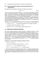
The first characterization of a Poisson process, that is, as a random counting measure,
provides an alternative way of generating such processes, which works also in the multidi-
mensional case. In particular (see the end of Section 1.1 l), the following procedure can be
used to generate a homogeneous Poisson process with rate
X
on any set A with “volume”
In
U,
and declare an arrival.
IAl.

GENERATING POISSON PROCESSES
71
Algorithm
2.6.2
(Generating an n-Dimensional Poisson Process)
1.
Generate a Poisson random variable
N
-
Poi(X
IAI).
2.
Given
N
=
n,
draw
n.
points independently and uniformly in
A.
Return these as the
A
nonhomogeneous Poissonprocess
is a counting process
N
=
{
Nt,
t
>

0)
for which
the number of points in nonoverlapping intervals are independent
-
similar to the ordinary
Poisson process
-
but the rate at which points arrive is
time dependent.
If X(t) denotes
the rate at time t, the number of points in any interval
(b,
c)
has a Poisson distribution with
mean
sl
A(t) dt.
Figure
2.9
illustrates a way to construct such processes. We first generate a two-
dimensional homogeneous Poisson process on the strip
{
(t,
z),
t
>
0,O
<
z
<

A},
with
constant rate
X
=
max
A(t),
and then simply project all points below the graph
of
A(t) onto
the t-axis.
points
of
the Poissonprocess.
f
Figure
2.9
Constructing
a
nonhomogeneous Poisson process.
Note that the points of the two-dimensional Poisson process can be viewed as having a
time and space dimension. The arrival epochs form a one-dimensional Poisson process with
rate
A,
and the positions are uniform on the interval
[0,
A].
This suggests the following al-
ternative procedure for generating nonhomogeneous Poisson processes: each arrival epoch
of

the one-dimensional homogeneous Poisson process is rejected (thinned) with probability
1
-
w,
where
T,
is the arrival time
of
the n-th event. The surviving epochs define the
desired nonhomogeneous Poisson process.
Algorithm
2.6.3
(Generating a Nonhomogeneous Poisson Process)
1.
Set
t
=
0,
n
=
0
and
i
=
0.
2.
Increase
i
by
1.

3.
Generate an independent random variable
U,
-
U(0,l).
4.
Set
t
=
t
-
4
In
u,.
5.
Ift
>
T,
stop; otherwise, continue.
6.
Generate an independent random variable
V,
-
U(0,l).
7.
IfV,
<
-"t;"'
,
increase

n
by
I
andset
T,,
=
t.
Go to Step
2.
72
RANDOM
NUMBER,
RANDOM
VARIABLE,
AND
STOCHASTIC
PROCESS
GENERATION
2-
2.7 GENERATING MARKOV CHAINS AND MARKOV JUMP PROCESSES
**
a*aW
.a
*
*-
a-
We now discuss how to simulate a Markov chain
XO, X1, X2,
.
.

.
,
X,.
To
generate a
Markov chain with initial distribution
do)
and transition matrix
P,
we can use the procedure
outlined in Section2.5 for dependentrandom variables. That is, first generate
XO
from
do).
Then, given
XO
=
ZO,
generate
X1
from the conditional distribution of
XI
given
XO
=
ZO;
in other words, generate
X1
from the zo-th row of
P.

Suppose
X1
=
z1.
Then, generate
X2
from the sl-st row of
P,
and
so
on. The algorithm for a general discrete-state Markov
chain with a one-step transition matrix
P
and an initial distribution vector
T(O)
is as follows:
Algorithm
2.7.1
(Generating a Markov Chain)
1.
Draw
Xofrorn
the initialdistribution
do),
Set
t
=
0.
2.
Draw

Xt+l
from the distribution corresponding
to
the Xt-th mw of
P.
3.
Set
t
=
t
+
1
andgo
to Step
2.
-2-
-4-
EXAMPLE
2.9
Random Walk on the Integers
ma
a
s
saw
0
sla
0
Consider the random walk on the integers in Example
1.10.
Let

XO
=
0
(that is, we
start at
0).
Suppose the chain is at some discrete time
t
=
0,
1,2
. .
.
in state
i.
Then, in
Step 2 of Algorithm
2.7.1,
we simply need to draw from a two-point distribution with
mass
p
and
q
at
i
+
1
and
i
-

1,
respectively. In other words, we draw
It
N
Ber(p)
and set
Xt+l
=
Xt
+
2Zt
-
1.
Figure
2.10
gives a typical sample path for the case
where
p
=
q
=
1/2.
6-
4.
Figure
2.10
Random
walk
on the integers, with
p

=
q
=
1/2.
2.7.1 Random Walk on a Graph
As a generalization of Example
2.9,
we can associate a random walk with any graph
G,
whose state space is the vertex set
of
the graph and whose transition probabilities from
i
to
j
are equal to
l/d,,
where
d,
is the degree of
i
(the number of edges out of
i).
An important
GENERATING MARKOV CHAINS AND MARKOV JUMP PROCESSES
73
property
of
such random walks is that they are time-reversible. This can be easily verified
from Kolmogorov’s criterion (1.39). In other words, there is no systematic “looping”.

As
a consequence, if the graph
is
connected and if the stationary distribution
{m,}
exists
-
which is the case when the graph
is
finite
-
then the local balance equations hold:
Tl
p,,
=
r,
PI,
.
(2.39)
When
p,,
=
p,,
for all
i
and
j,
the random walk is said to be
symmetric.
It follows

immediately from (2.39) that in this case the equilibrium distribution is uniform over the
state space
&.
H
EXAMPLE
2.10 Simple Random
Walk
on
an
n-Cube
We want to simulate a random walk over the vertices of the n-dimensional hypercube
(or simply n-cube); see Figure 2.1 1 for the three-dimensional case.
Figure
2.11
random.
At each
step,
one
of
the
three neighbors
of
the currently
visited
vertex
is
chosen
at
Note that the vertices of the n-cube are of the form
x

=
(21
,
. .
.
,
zn),
with
zi
either
0
or
1. The set of all
2“
of these vertices
is
denoted
(0,
1)”.
We generate a
random walk
{Xt,
t
=
0,1,2,.
.
.}
on
(0,
l}n

as follows. Let the initial state
XO
be arbitrary, say
XO
=
(0,.
.
.
,O).
Given
Xt
=
(~~1,.
.
.
,ztn).
choose randomly a
coordinate
J
according to the discrete uniform distribution on the set
{
1,
. . .
,
n}.
If
j
is
the outcome, then replace
zjn

with
1
-
xjn.
By doing
so
we obtain at stage
t
+
1
Xt+l
=
(5tl, ,l-~tj,zt(j+l)r ,5tn)
1
and
so
on.
2.7.2
Generating Markov
Jump
Processes
The generation
of
Markov jump processes is quite similar to the generation of Markov
chains above. Suppose
X
=
{
Xt,
t

2
0)
is a Markov jump process with transition rates
{qE3}.
From Section 1.12.5, recall that the Markov jump process jumps from one state to
another according to a Markov chain
Y
=
{
Y,}
(thejump chain), and the time spent in each
state
z
is exponentially distributed with a parameter that may depend on
i.
The one-step
transition matrix, say
K,
of
Y
and the parameters
(9,)
of the exponential holding times
can be found directly from the
{qE3}.
Namely,
q,
=
C,
qV

(the sum of the transition rates
out of
i),
and
K(i,j)
=
q,,/9,
for
i
#
j
(thus, the probabilities are simply proportional to
74
RANDOM NUMBER, RANDOM VARIABLE, AND STOCHASTIC PROCESS GENERATION
the rates). Note that
K(i,
i)
=
0.
Defining the holding times as
A1,
Az,
. . .
and the jump
times as
2'1,
Tz,
.
.
.

,
the algorithm is now as follows.
Algorithm
2.7.2
(Generating a Markov Jump Process)
1.
Initialize
TO.
Draw
Yo
from the initial distribution
do).
Set XO
=
YO.
Set
n
=
0.
2.
Draw
An+l
from
Exp(qy,).
3.
Set
Tn+l
=
T,,
+

An+l.
4.
SetXt
=
Yn
forTn
6
t
<
Tn+i.
5.
Draw
Yn+l
from the distribution corresponding to the Yn-th row of
K,
set
'n
=
n
+
1,
and
go
to Step
2.
2.8 GENERATING RANDOM PERMUTATIONS
Many Monte Carlo algorithms involve generating random permutations, that is, random
ordering of the numbers 1,2,
.
. .

,
n,
for some fixed
n.
For examples of interesting problems
associated with the generation of random permutations, see, for instance, the traveling
salesman problem in Chapter
6,
the permanent problem in Chapter
9,
and Example
2.1
1
below.
Suppose we want to generate each of the
n!
possible orderings with equal probability.
We present two algorithms that achieve this. The first one is based on the ordering of a
sequence of
n
uniform random numbers. In the second, we choose the components of the
permutation consecutively. The second algorithm is faster than the first.
Algorithm
2.8.1
(First Algorithm for Generating Random Permutations)
1.
Generate
U1,
U2,.
. . ,

Un
N
U(0,l)
independently
2.
Arrange these in increasing order.
3.
The indices of the successive ordered values form the desiredpermutation.
For example, let
n
=
4 and assume that the generated numbers
(U1,
Uz,
U,,
U4)
are
(0.7,0.3,0.5,0.4). Since
(UZ,
U4,
U3,Ul)
=
(0.3,0.4,0.5,0.7) is the ordered sequence,
the resulting permutation is (2,4,3,1). The drawback of this algorithm is that it requires
ordering a sequence of
n
random numbers, which requires
n
Inn
comparisons.

As we mentioned, the second algorithm is based on the idea of generating the components
of the random permutation one by one. The first component is chosen randomly (with
equal probability) from 1,.
.
.
,
n.
Next, the second component is randomly chosen from
the remaining numbers, and
so
on. For example, let
n
=
4.
We draw component
1
from
the discrete uniform distribution on
{
1,2,3,4}. Suppose we obtain
2.
Our permutation
is thus
of
the form (2,
.,
.,
.).
We next generate from the three-point uniform distribution
on

{
1,3,4}.
Assume that
1
is chosen. Thus,
our
intermediate result for the permutation
is (2,1,
.,
.).
Finally, for the third component, choose either
3
or 4 with equal probability.
Suppose we draw
4.
The resulting permutation is (2,1,4,3). Generating a random variable
X
from a discrete uniform distribution on
{
51,
. .
.
,
zk}
is done efficiently by first generating
I
=
[k
UJ
+

1,
with
U
-
U(0,l) and returning
X
=
51.
Thus, we have the following
algorithm.
PROBLEMS
75
Algorithm
2.8.2
(Second Algorithm for Generating Random Permutations)
I.
Set9={1,
,
n}.Leti=l.
2.
Generate
Xi
from the discrete uniform distribution
on
9.
3.
Remove
Xi
from
9.

4.
Set
i
=
i
+
1.
Ifi
<
n,
go
to Step
2.
5.
Deliver
(XI,
. .
.
,
X,)
as the desiredpermutation.
Remark
2.8.1
To further improve the efficiency of the second random permutation algo-
rithm, we can implement it as follows: Let
p
=
(pi,.
. .
,pn)

be a vector that stores the
intermediate results of the algorithm at the i-th step. Initially, let
p
=
(1,
. . .
,
n).
Draw
X1
by uniformly selecting an index
I
E
{
1,
.
. .
,
n},
and return
X1
=
pl.
Then
swap
X1
and
p,
=
n.

In the second step, draw
X2
by uniformly selecting
I
from
{
1,
.
.
.
,
n
-
l},
return
X,
=
p1
and swap it with
pn-l,
and
so
on. In this way, the algorithm requires the generation
of only
n
uniform random numbers (for drawing from
{
1,2,
.
.

.
,
k},
k
=
n,
n
-
1,
. .
.
,2)
and
n
swap operations.
EXAMPLE
2.11
Generating a Random Tour in
a
Graph
Consider a weighted graph
G
with
n
nodes, labeled
1,2,
. .
.
,
n.

The nodes repre-
sent cities, and the edges represent the roads between the cities. The problem is to
randomly generate a
tour
that visits all the cities exactly once except for the starting
city, which is also the terminating city. Without
loss
of generality, let
us
assume that
the graph is complete, that is, all cities are connected. We can represent each tour
via a permutation of the numbers
1,
.
. . ,
n,
For example, for
n
=
4,
the permutation
(1,3,2,4)
represents the tour
1
-+
3
-+
2
-+
4

-+
1.
More generally, we represent a tour via a permutation
x
=
(21,
. .
.
,
5,)
with
21
=
1,
that is, we assume without
loss
of
generality that we start the tour at city number
1.
To
generate a random tour uniformly on
X,
we can simply apply Algorithm
2.8.2.
Note that the number
of
all possible tours of elements in the set of all possible tours
X
is
IZI

=
(n
-
l)!
(2.40)
PROBLEMS
2.1
uniform distribution with pdf
Apply the inverse-transform method to generate a random variable from the discrete
z
=
0,1,.
.
.,n
0
otherwise.
f(x)
=
2.2
method.
2.3
method.
Explain how to generate from the
Beta(1,
p)
distribution using the inverse-transform
Explain how to generate from the
Weib(cu,
A)
distribution using the inverse-transform

76
RANDOM
NUMBER.
RANDOM
VARIABLE,
AND
STOCHASTIC PROCESS
GENERATION
2.4
transform method.
2.5
Explain how to generate from the
Pareto(cY,
A)
distribution using the inverse-
Many families of distributions are of
location-scale
type. That is, the cdf has the
form
where
p
is called the
location
parameter and
a
the
scale
parameter, and
FO
is a fixed cdf

that does not depend on
p
and
u.
The
N(p,
u2)
family of distributions
is
a good example,
where
FO
is the standard normal cdf. Write F(x;
p,
a)
for F(x). Let
X
-
FO
(that is,
X
-
F(x;
0,l)).
Prove that
Y
=
p
+
u

X
-
F(z;
pl
a).
Thus, to sample from any cdf in
a location-scale family, it suffices to know how to sample from
Fo.
2.6 Apply the inverse-transform method to generate random variables from a
Laplace
distribution
(that
is,
a shifted two-sided exponential distribution) with pdf
2.7
value distribution,
which has cdf
Apply the inverse-transform method to generate a random variable from the
extreme
2.8
Consider the triangular random variable with pdf
ifx
<
2aorx
2
2b
fo
if 2a
<
x

<
a
+
b
(2b
-
X)
ifa+
b
<
x
<
2b
I-
(b
-
a)2
a)
Derive the corresponding cdf
F.
b)
Show that applying the inverse-transform method yields
2a+(b-a)m ifO<U<$
26
+
(a
-
b)
dm
X={

if
<
U
<
1
.
2.9
piecewise-constant pdf
Present an inverse-transform algorithm for generating a random variable from the
where
Ci
0
and
xo
<
XI
<
. . .
<
x,-1
<
x,
PROBLEMS
77
2.10
Let
where
C,
0
and

xo
<
x1
<

<
xn-l
<
2,.
a)
Let
Fi
=
xi.,,
sz-
Cj
u
du,
a
=
1,
.
. . ,
n.
Show that the cdf
F
satisfies
Ci
F(z)=Fi-l+-(zZ-x~-,),
xi-l <x<xi,

i=l,
,
n.
2
b)
Describe an inverse-transform algorithm for random variable generation from
f
(x).
2.1 1
A
random variable is said to have a
Cuuchy
distribution if its pdf is given by
(2.41)
Explain how one can generate Cauchy random variables using the inverse-transform method.
2.12
If
X
and
Y
are independent standard normal random variables, then
2
=
X/Y
has
a Cauchy distribution. Show this. (Hint: first show that if
U
and
V
>

0
are continuous
random variables with joint pdf
fu,~,
then the pdf
of
W
=
U/V
is given by
fw(w)
=
2.13
2.14
ing random variables from the following normal (Gaussian) mixture pdf
J,"
fu,v(w
'u,
.)
'u
dv.)
Verify the validity of the composition Algorithm
2.3.4.
Using the composition method, formulate and implement an algorithm for generat-
where
cp
is the pdf of the standard normal distribution and
(plrp2,p3)
=
(1/2,1/3,1/6),

(~1,
a2,
~3)
=
(-1,O,
11,
and
(bi, b2, b3)
=
(1/4,1,1/2).
2.15
Verify that
C
=
in Figure
2.5.
2.16
2.17
XU'/"
-
Gamma(cr,
1).
Prove this.
2.18
Prove that if
X
-
Gamma(&,
l),
then

X/X
-
Gamma(&,
A).
Let
X
-
Gamma(1
+
a,
1)
and
U
-
U(0,l)
be independent.
If
a
<
1,
then
If
Y1
-
Gamma(a,
l),
Y2
-
Gamma@,
l),

and
Yl
and
Y2
are independent, then
is
Beta(&,
p)
distributed. Prove this.
2.19
Devise an acceptance-rejection algorithm for generating a random variable from the
pdf
f
given in
(2.20)
using an
Exp(X)
proposal distribution. Which
X
gives the largest
acceptance probability?
2.20
The pdf of the truncated exponential distribution with parameter
X
=
1
is
given by
e-=
f(x)

=
->
O<x<a.
78
RANDOM NUMBER, RANDOM VARIABLE, AND STOCHASTIC PROCESS GENERATION
a)
Devise an algorithm for generating random variables from this distribution using
the inverse-transform method.
b)
Construct a generation algorithm that uses the acceptance-rejection method with
an
Exp(X)
proposal distribution.
c)
Find the efficiency of the acceptance-rejection method for the cases
a
=
1,
and
a
approaching zero and infinity.
Let the random variable
X
have pdf
2.21
4’
O<x<l
x-$, 1<2<2.
f(x)
=

Generate a random variable from
f(x),
using
a)
the inverse-transform method,
b)
the acceptance-rejection method, using the proposal density
2.22
Let the random variable
X
have pdf
Generate a random variable from
,f(z),
using
a)
the inverse-transform method
b)
the acceptance-rejection method, using the proposal density
8
5
2
g(5)=25x’ o<x<-
2.23
Let
X
have a truncated geometric distribution, with pdf
f(x)
=
cp(1
-

p)5-1,
5
=
1,.
.
.
,
n
,
where
c
is a normalization constant. Generate a random variable from
f(x),
using
a)
the inverse-transform method,
b)
the acceptance-rejection method, with
G(p)
as the proposal distribution. Find the
2.24
Generate a random variable
Y
=
min,=I,
.,m
max3=l
,.
.
,,.

{ X,j},
assuming that
the variables
X,,,
i
=
1,.
.
. ,
m,
j
=
1,.
. .
,
T,
are iid with common cdf
F(x),
using the
inverse-transform method. (Hint: use the results for the distribution of order statistics in
Example
2.3.)
2.25
Generate
100
Ber(0.2)
random variables three times and produce bar graphs similar
to those in Figure
2.6.
Repeat for

Ber(0.5).
2.26
Generate a homogeneous Poisson process with rate
100
on the interval
[0,1].
Use
this to generate a nonhomogeneousPoisson process on the same interval, with rate function
efficiency of the acceptance-rejection method for
R
=
2
and
R
=
00.
~(t)
=
100
sin2(10t),
t
2
o
.
PROBLEMS
79
2.27
Generate and plot a realization of the points of a two-dimensional Poisson process
withrateX
=

2onthesquare[0,5]x [0;5].
Howmanypointsfallinthesquare(1,3]
x
[1,3]?
How many do you expect to fall in this square?
2.28
Write a program that generates and displays
100
random vectors that are uniformly
distributed within the ellipse
5
z2
+
21
z
y
+
25
y2
=
9
.
2.29
Implement both random permutation algorithms in Section 2.8. Compare their
performance.
2.30
Consider a random walk on the undirected graph in Figure 2.12.
For
example, if the
random walk at some time is in state

5,
it will jump to
3,4,
or
6
at the next transition, each
with probability
1/3.
1
3
5
2
4
6
Figure
2.12
A
graph.
a)
Find the one-step transition matrix
for
this Markov chain.
b)
Show that the stationary distribution is given by
7r
=
(i,
i,
g,
5,

i,
i).
c)
Simulate the random walk on a computer and verify that in the long run, the
proportion
of
visits to the various nodes is in accordance with the stationary
distribution.
2.31
Generate various sample paths
for
the random walk on the integers for
p
=
1/2
and
p
=
213.
2.32
Consider the
M/M/1
queueing system of Example 1.13. Let
Xt
be the number
of customers in the system at time
t.
Write a computer program to simulate the stochastic
process
X

=
{
X,}
by viewing
X
as a Markov jump process, and applying Algorithm 2.7.2.
Present sample paths of the process for the cases
X
=
1,
p
=
2 and
X
=
10,
p
=
11.
Further
Reading
Classical references on random number generation and random variable generation are [3]
and [2].
Other references include
[4],
[7], and [lo] and the tutorial in
[9].
A good new
reference is
[

11.
80
RANDOM
NUMBER.
RANDOM
VARIABLE, AND
STOCHASTIC
PROCESS
GENERATION
REFERENCES
1.
S.
Asmussen and
P.
W. Glynn.
Stochastic Simulation.
Springer-Verlag, New York, 2007.
2. L. Devroye.
Non-Uniform Random Variate Generation.
Springer-Verlag. New York, 1986.
3.
D.
E. Knuth.
The Art of Computer Programming,
volume
2:
Seminumerical Algorithms.
Addison-Wesley, Reading, 2nd edition, 198
1.
edition, 2000.

1990.
4.
A. M. Law and W.
D.
Kelton.
Simulation Modeling and Analysis.
McGraw-Hill, New York, 3rd
5.
P.
L'Ecuyer. Random numbers
for
simulation.
Communications
of
the ACM,
33( l0):85-97,
6. D.
H.
Lehmer. Mathematical methods in large-scale computing units.
Annals of the Computation
7. N. N. Madras.
Lectures
on
Monte Carlo Methods.
American Mathematical Society, 2002.
8.
G.
Marsaglia and W. Tsang. A simple method
for
generating gamma variables.

ACM Transac-
9.
B.
D. Ripley. Computer generation
of
random variables: A tutorial.
International Statistical
Laboratory ofHarvard Universiy,
26:141-146, 1951.
tions on Mathematical Sofiare,
26(3):363-372,2000.
Review,
51:301-319, 1983.
10.
S.
M. Ross.
Simularion.
Academic
Press,
New York, 3rd edition, 2002.
11. A.
J.
Walker. An efficient method
for
generating discrete random variables with general distri-
butions.
ACM Transactions
on
Mathematical Sofiare,
3:253-256, 1977.

CHAPTER
3
SIMULATION
OF
DISCRETE-EVENT
SYSTEMS
Computer simulation has long served as an important tool in a wide variety of disciplines:
engineering, operations research and management science, statistics, mathematics, physics,
economics, biology, medicine, engineering, chemistry, and the social sciences. Through
computer simulation, one can study the behavior of real-life systems that are too difficult
to examine analytically. Examples can be found in supersonic jet flight, telephone com-
munications systems, wind tunnel testing, large-scale battle management (e.g., to evaluate
defensive or offensive weapons systems), or maintenance operations (e.g., to determine the
optimal size
of
repair crews), to mention a few. Recent advances in simulation methodolo-
gies, software availability, sensitivity analysis, and stochastic optimization have combined
to
make simulation one
of
the most widely accepted and used tools in system analysis and
operations research. The sustained growth in size and complexity of emerging real-world
systems (e.g., high-speed communication networks and biological systems) will undoubt-
edly ensure that the popularity
of
computer simulation continues to grow.
The aim of this chapter is to provide a brief introduction to the art and science of computer
simulation, in particular with regard
to
discrete-event systems. The chapter is organized

as follows: Section
3.1
describes basic concepts such as systems, models, simulation, and
Monte Carlo methods. Section
3.2
deals with the most fundamental ingredients of discrete-
event simulation, namely, the simulation clock and the event list. Finally, in Section
3.3
we
further explain the ideas behind discrete-event simulation via a number
of
worked examples.
Simulation and the Monte
Carlo
Method, Second Edition.
By R.Y. Rubinstein
and
D.
P.
Kroese
Copyright
@
2007
John Wiley
&
Sons,
Inc.
81
82
SIMULATION

OF
DISCRETE-EVENT
SYSTEMS
3.1
SIMULATION MODELS
By a
system
we mean a collection of related entities, sometimes called
components
or
elements,
forming a complex whole. For instance, a hospital may be considered a system,
with doctors, nurses, and patients as elements. The elements possess certain characteristics
or
attributes
that take on logical
or
numerical values. In our example, an attribute may be
the number of beds, the number of X-ray machines, skill level, and
so
on. Typically, the
activities of individual components interact over time. These activities cause changes in the
system’s state. For example, the state of a hospital’s waiting room might be described by
the number of patients waiting for a doctor. When a patient arrives at the hospital
or
leaves
it,
the system jumps to a new state.
We shall be solely concerned with
discrete-eventsystems,

to wit, those systems in which
the state variables change instantaneously through jumps at discrete points in time, as op-
posed to
continuous systems,
where the state variables change continuously with respect
to time. Examples of discrete and continuous systems are, respectively, a bank serving
customers and a car moving on the freeway. In the former case, the number of waiting
customers is a piecewise constant state variable that changes only when either a new cus-
tomer arrives at the bank
or
a customer finishes transacting his business and departs from
the bank; in the latter case, the car’s velocity is a state variable that can change continuously
over time.
The first step in studying a system is to build a model from which one can obtain
predictions concerning the system’s behavior. By a
model
we mean an abstraction of
some real system that can be used to obtain predictions and formulate control strategies.
Often such models are mathematical (formulas, relations) or graphical in nature. Thus, the
actual physical system is translated
-
through the model
-
into a mathematical system.
In order to be useful, a model must necessarily incorporate elements of two conflicting
characteristics: realism and simplicity. On the one hand, the model should provide a
reasonably close approximation to the real system and incorporate most
of
the important
aspects of the real system. On the other hand, the model must not be

so
complex
as
to
preclude its understanding and manipulation.
There are several ways to assess the validity of a model. Usually, we begin testing
a model by reexamining the formulation of the problem and uncovering possible flaws.
Another check on the validity of a model is to ascertain that all mathematical expressions
are dimensionally consistent. A third useful test consists of varying input parameters and
checking that the output from the model behaves in a plausible manner. The fourth
test
is
the so-called
retrospective
test. It involves using historical data to reconstruct the past and
then determining how well the resulting solution would have performed if it had been used.
Comparing the effectiveness of this hypothetical performance with what actually happens
then indicates how well the model predicts reality. However, a disadvantage of retrospective
testing is that it uses the same data as the model. Unless the past
is
a representative replica
of the future, it is better not to resort to this test at all.
Once a model
for
the system at hand has been constructed, the next step is to derive
a
solution from this model.
To
this end, both
analytical

and
numerical
solutions methods
may be invoked. An analytical solution is usually obtained directly from its mathematical
representation
in
the form of formulas. A numerical solution
is
generally an approximation
via a suitable approximation procedure. Much of this book deals with numerical solution
and estimation methods obtained via computer simulation. More precisely, we use
stochas-
tic computer simulation
-
often called
Monte Carlo simulation
-
which includes some
randomness in the underlying model, rather than deterministic computer simulation. The
SIMULATION
MODELS
83
term
Monte
Curlo
was used by von Neumann and Ulam during World War
I1
as a code
word for secret work at
Los

Alamos on problems related to the atomic bomb. That work
involved simulation of random neutron diffusion in nuclear materials.
Naylor et al.
[7]
define
simulation
as follows:
Simulation is a numerical technique for conducting experiments
on
a digital computer:
which involves certain types of mathematical and logical models that describe the
behavior
of
business or economic systems (or some component thereon over extended
period ofreal time.
The following list of typical situations should give the reader some idea of where simu-
lation would be an appropriate tool.
0
The system may be
so
complex that a formulation in terms of a simple mathematical
equation may be impossible. Most economic systems fall into this category. For
example, it is often virtually impossible
to
describe the operation of a business firm,
an industry, or an economy in terms of a few simple equations. Another class of
problems that leads to similar difficulties is that of large-scale, complex queueing
systems. Simulation has been an extremely effective tool for dealing with problems
of this type.
Even if a mathematical model can be formulated that captures the behavior of some

system of interest, it may not be possible to obtain a solution to the problem embodied
in the model by straightforward analytical techniques. Again, economic systems and
complex queueing systems exemplify this type of difficulty.
0
Simulation may be used as a pedagogical device for teaching both students and
practitioners basic skills in systems analysis, statistical analysis, and decision making.
Among the disciplines in which simulation has been used successfully for this purpose
are business administration, economics, medicine, and law.
The formal exercise of designing a computer simulation model may be more valuable
than the actual simulation itself. The knowledge obtained in designing a simulation
study serves to crystallize the analyst’s thinking and often suggests changes in the
system being simulated. The effects of these changes can then be tested via simulation
before implementing them in the real system.
0
Simulation can yield valuable insights into the problem of identifying which variables
are important and which have negligible effects on the system, and can shed light on
how these variables interact; see Chapter
7.
0
Simulation can be used to experiment with new scenarios
so
as to gain insight into
system behavior under new circumstances.
Simulation provides an
in
vitro
lab, allowing the analyst to discover better control of
the system under study.
0
Simulation makes it possible to study dynamic systems in either real, compressed, or

expanded time horizons.
Introducing randomness in a system can actually help solve many optimization and
counting problems; see Chapters
6
-
9.
84
SIMULATION
OF
DISCRETE-EVENT
SYSTEMS
As
a modeling methodology, simulation is by no means ideal. Some of its shortcomings
and various caveats are: Simulation provides
statistical estimates
rather than
exact
charac-
teristics and performance measures of the model. Thus, simulation results are subject to
uncertainty and contain experimental errors. Moreover, simulation modeling is typically
time-consuming and consequently expensive in terms of analyst time. Finally, simulation
results, no matter how precise, accurate, and impressive, provide consistently useful infor-
mation about the actual system
only
if the model is a valid representation of the system
under study.
3.1
.I
Classification
of

Simulation
Models
Computer simulation models can be classified in several ways:
I.
Static versus Dynamic Models.
Static models are those that do not evolve over time
and therefore do not represent the passage of time. In contrast, dynamic models
represent systems that evolve over time (for example, traffic light operation).
2.
Deterministic versus Stochastic Models.
If a simulation model contains
only
deter-
ministic (i.e., nonrandom) components, it is called
deterministic.
In a deterministic
model, all mathematical and logical relationships between elements (variables) are
fixed in advance and not subject to uncertainty.
A
typical example is a complicated
and analytically unsolvable system of standard differential equations describing, say,
a chemical reaction. In contrast, a model with at least one random input variable
is called a
stochastic
model. Most queueing and inventory systems are modeled
stochastically.
3.
Continuous versus Discrete Simulation Models.
In discrete simulation models the
state variable changes instantaneously at discrete points in time, whereas in contin-

uous
simulation models the state changes continuously over time.
A
mathematical
model aiming to calculate a numerical solution for a system of differential equations
is an example of continuous simulation, while queueing models are examples of
discrete simulation.
This book deals with discrete simulation and in particular with
discrete-event simulation
(DES) models. The associated systems are driven by the occurrence
of
discrete events,
and their state typically changes over time. We shall further distinguish between so-called
discrete-event static systems
(DESS) and
discrete-event dynamic systems
(DEDS). The
fundamental difference between DESS and DEDS is that the former do not evolve over
time, whereas the latter do.
A
queueing network is a typical example of a DEDS.
A
DESS
usually involves evaluating (estimating) complex multidimensional integrals or sums via
Monte Carlo simulation.
Remark
3.1.1
(Parallel Computing)
Recent advances in computer technology have en-
abled the use

ofparallel
or
distributedsimulation,
where discrete-event simulation is carried
out on multiple linked (networked) computers, operating simultaneously in a cooperative
manner. Such an environment allows simultaneous distribution of different computing tasks
among the individual processors, thus reducing the overall simulation time.
SIMULATION
CLOCK
AND
EVENT
LIST
FOR DEDS
85
3.2
SIMULATION CLOCK AND EVENT LIST
FOR
DEDS
Recall that
DEDS
evolve over time. In particular, these systems change their state only at a
countable number of time points. State changes are triggered by the execution of simulation
events occurring at the corresponding time points. Here, an
event
is a collection
of
attributes
(values, types, flags, etc.), chief among which are the
event occurrence time
-

or simply
event time
-
the
event
type,
and an associated algorithm to execute state changes.
Because of their dynamic nature,
DEDS
require a time-keeping mechanism to advance
the simulation time from one event to another as the simulation evolves over time. The
mechanism recording the current simulation time is called the
simulation
clock.
To
keep
track of events, the simulation maintains a list
of
all pending events. This list is called the
event list,
and its task is to maintain all pending events in
chronological
order. That is,
events are ordered by their time of occurrence. In particular, the most imminent event is
always located at the head of the event list.
Clock
Event List
Figure
3.1
The advancement

of
the simulation clock and event list.
The situation is illustrated in Figure
3.1.
The simulation starts by loading the initial
events into the event list (chronologically ordered), in this case four events. Next, the most
imminent event
is
unloaded from the event list for execution, and the simulation clock is
advanced to its occurrence time,
1.234.
After this event
is
processed and removed, the
clock is advanced to the next event, which occurs at time
2.354.
In the course
of
executing
a current event, based on its type, the state
of
the system is updated, and future events are
possibly generated and loaded into (or deleted from) the event list. In the above example,
the third event
-
of type
C,
occurring at time
3.897
-

schedules a new event of type
E
at
time
4.23
1.
The process of unloading events from the event list, advancing the simulation clock, and
executing the next most imminent event terminates when some specific stopping condition
is met
-
say, as soon
as
a prescribed number of customers departs from the system. The
following example illustrates this
next-event time advance
approach.
86
SIMULATION
OF
DISCRETE-EVENT
SYSTEMS
EXAMPLE3.1
Money enters a certain bank account in two ways: via frequent small payments and
occasional large payments. Suppose that the times between subsequent frequent pay-
ments are independent and uniformly distributed on the continuous interval
[7,
101 (in
days); and, similarly, the times between subsequent occasional payments are indepen-
dent and uniformly distributed on [25,35]. Each frequent payment is exponentially
distributed with a mean of

16
units (say, one unit is
$1000),
whereas occasional pay-
ments are always of size
100.
It is assumed that all payment intervals and sizes are
independent. Money is debited from the account at times that form a Poisson process
with rate
1
(per day), and the amount debited is normally distributed with mean
5
and
standard deviation
1.
Suppose that the initial amount of money in the bank account
is 150 units.
Note that the state of the system -the account balance
-
changes only at discrete
times.
To
simulate this DEDS, one need only keep track of when the next frequent
and occasional payments occur, as well as the next withdrawal. Denote these three
event types by 1.2, and 3, respectively. We can now implement the event list simply
as a
3
x
2 matrix, where each row contains the event time and the event type. After
each advance of the clock, the current event time

t
and event type
i
are recorded and
the current event is erased. Next, for each event type
i
=
1,2,3 the same type of
event is scheduled using its corresponding interval distribution. For example, if the
event type is 2, then another event of type
2
is scheduled at a time
t
+
25
+
10
U,
where
U
-
U[O,
11.
Note that this event can be stored in the same location as the
current event that was just erased. However, it is crucial that the event list is then
resorted to put the events in chronological order.
A realization of the stochastic process
{
Xt,
0

<
t
<
400},
where
Xt
is the account
balance at time
t,
is given in Figure 3.2, followed by a simple Matlab implementation.
200
150
-
0
0
0
tft
7
x
100
8
m
n
=
50
Y
-
m
z
0

::I:
Figure
3.2
A
realization
of
the simulated account balance process.
DISCRETE-EVENT
SIMULATION 87
Matlab
Program
clear all;
T
=
400;
x
=
150; %initial mount
of
money.
xx
=
C1501; tt
=
LO];
t=O;
ev-list
=
inf*ones(3,2); %record time, type
ev-list(1,

:)
=
[7
+
3*rand, 11
;
%schedule type
1
event
ev-list(2,
:)
=
[25
+
lO*rand,21
;
%schedule type
2
event
ev-list
(3,
:
)
=
[-log(rand) ,3]
;
%schedule type
3
event
ev-list

=
sortrows(ev-list,l);
%
sort event list
while t
<
T
t
=
ev-list(l,l);
ev-type
=
ev-list (1,2)
;
switch ev-type
case
1
x
=
x
+
16*-log(rand);
ev-list(1,
:)
=
[7
+
3*rand
+
t,

11
;
x
=
x
+
100;
ev-list
(1,
:)
=
[25
+
10*rand
+
t,
21
;
x
=
x
-
(5
+
randn);
ev-list(1,
:)
=
[-log(rand)
+

t,
31
;
case
2
case
3
end
ev-list
=
sortrows(ev-list,l);
%
sort event list
xx
=
[xx,xl
;
tt
=
[tt,tl;
end
plot (tt
,xx)
3.3
DISCRETE-EVENT SIMULATION
As
mentioned,
DES
is the standard framework for the simulation of a large class of models
in which the system

state
(one or more quantities that describe the condition
of
the system)
needs to be observed only at certain critical epochs (event times). Between these epochs, the
system state either stays the same or changes in a predictable fashion. We further explain
the ideas behind
DES
via two more examples.
3.3.1
Tandem
Queue
Figure
3.3
depicts a simple queueing system, consisting of two queues in tandem, called a
(Jackson)
tandem
queue.
Customers arrive at the first queue according to a Poisson process
with rate
A.
The service time of a customer at the first queue
is
exponentially distributed
with rate
111.
Customers who leave the first queue enter the second one. The service time in
the second queue has an exponential distribution with rate
pz.
All

interarrival and service
times are independent.
Suppose we are interested in the number
of
customers,
Xt
and
Yt,
in the first and second
queues, respectively, where we regard a customer who is being served as part of the queue.
Figure
3.4
depicts a typical realization of the queue length processes
{Xt,
t
>
0)
and
{
Yt,
t
>
0},
obtained via
DES.
88 SIMULATION
OF
DISCRETE-EVENT SYSTEMS
3
2.5

1
Queue
1
Queue
2
L-m
Figure
3.3
A
Jackson tandem queue.
t
0
0.5
1
1.5
2
2.5
3
3.5
4
4.5
5
t
Figure
3.4
A
realization of the queue length processes
(Xt
,
t

2
0)
and
(Yi,
t
2
0).
Before we discuss how to simulate the queue length processes via DES, observe that,
indeed, the system evolves via a sequence of discrete events, as illustrated in Figure
3.5.
Specifically, the system state
(Xt,
K)
changes only at times of an arrival at the first queue
(indicated by A), a departure from the first queue (indicated by Dl), and a departure from
the second queue (D2).
A
DIAA D2 D1 A
I I
II
I
I I
I
I
Pt
Figure
3.5
departure
from
the second queue).

A
sequence
of
discrete-events
(A
=
anival, D1
=
departure from the
first
queue, D2
=
There are two fundamental approaches to DES, called the
event-oriented
and
pmcess-
oriented
approaches. The pseudocode for an event-oriented implementation of the tandem
queue is given
in
Figure
3.6.
The program consists of a main subroutine and separate
DISCRETE-EVENT SIMULATION
89
subroutines for each event. In addition, the program maintains an ordered list of scheduled
current and future events, the so-called
event
list.
Each event in the event list has an event

type
(‘A’,
‘Dl’, and ‘D2’) and an event
time
(the time at which the arrival or departure will
occur). The role
of
the main subroutine is primarily to progress through the event list and
to call the subroutines that are associated with each event type.
Main
1:
initialize:
Let
t
=
0,
x
=
0
and
y
=
0.
2:
Schedule ‘A’ at
t
+
Exp(X).
3:
while

TRUE
4:
5:
6:
switch
current event type
I:
case
‘A’: Call
Arrival
8:
case
‘Dl’: Call
Departurel
9:
case
‘D2’: Call
Departure2
10:
end
I
I:
12:
end
Get the first event in the event list
Let
t
be the time of this (now current) event
Remove the current event from the event list and sort the event list.
Figure

3.6
Main subroutine
of
an
event-oriented simulation program.
The role
of
the event subroutines is to update the system state and to schedule new events
into the event list. For example, an arrival event at time
t
will trigger another arrival event
at time
t
+
2,
with
2
-
Exp(X).
We write this, as in the Main routine, in shorthand as
t
+
Exp(X).
Moreover, if the first queue is empty, it will also trigger a departure event from
the first queue at time
t
+
Exp(p1).
Arrival
Schedule ‘A’

ifx=O
at
1:
+
Exp(X)
Schedule ‘Dl’
at
+
EXP(P1)
end
Z=Z+l
Departurel
z=x-l
ifx#O
Schedule ‘D
1
’
at
t
+
Exp(p1)
end
ifx=O
Schedule ‘D2’
at
t
+
EXP(PZ)
end
y=y+l

Departure2
r-
at
t
+
Exp(p2)
y=y-1
ify#O
Schedule ‘D2’
Figure
3.7
Event subroutines
of
an event-oriented simulation program
The process-oriented approach to
DES
is much more flexible than the event-oriented ap-
proach.
A
process-oriented simulation program closely resembles the actual processes that
drive the simulation. Such simulation programs are invariably written in an object-oriented
programming language, such as Java
or
C++. We illustrate the process-oriented approach
via our tandem queue example. In contrast to the event-oriented approach, customers,
90
SIMULATION
OF
DISCRETE-EVENT SYSTEMS
servers, and queues are now actual entities,

or
objects
in the program, that can be manip-
ulated. The queues are passive objects that can contain various customers (or be empty),
and the customers themselves can contain information such as their arrival and departure
times. The servers, however, are active objects
(processes),
which can interact with each
other and with the passive objects.
For
example, the first server takes a client out of the
first queue, serves the client, and puts her into the second queue when finished, alerting the
second server that a new customer has arrived if necessary. To generate the arrivals, we
define a
generator
process that generates a client, puts it in the first queue, alerts the first
server if necessary, holds for a random interarrival time (we assume that the interarrival
times are iid), and then repeats these actions to generate the next client.
As in the event-oriented approach, there exists an event list that keeps track of the current
and pending events. However, this event list now containspmcesses. The process at the top
of
the event list is the one that is currently active. Processes may ACTIVATE other processes
by putting them at the head of the event list. Active processes may HOLD their action for a
certain amount
of
time (such processes are put further up in the event list). Processes may
PASSIVATE altogether (temporarily remove themselves from the event list). Figure
3.8
lists the typical structure of a process-oriented simulation program for the tandem queue.
Main

1:
initialize:
create the two queues, the two servers and the generator
2:
ACTIVATE the generator
3:
HOLD(duration of simulation)
A.
STOP
Generator
I:
while
TRUE
2:
generate new client
3:
put client in the first queue
4:
if
server
1
is idle
5:
ACTIVATE server
1
6:
end
7:
HOLD(interarriva1 time)
8:

end
Server
1
I:
while
TRUE
2:
3:
PASSIVATE
4:
else
5:
6:
HOLD( service time)
7:
end
8:
put customer in queue
2
9:
if
server
2
is idle
10:
ACTIVATE server
2
11:
end
12:

end
if
waiting room is empty
get first customer from waiting
room
Figure
3.8
The structure of a process-oriented simulation program
for
the tandem queue. The
Server
2
process is similar
to
the Server
1
process, with lines
8-1
1
replaced with "remove customer
from system".
The collection of statistics, for example the waiting time
or
queue length, can be done by
different objects and at various stages in the simulation. For example, customers can record
their arrival and departure times and report
or
record them just before they leave the system.
There are many freely available object-oriented simulation environments nowadays, such
as SSJ, J-Sim, and C++Sim, all inspired by the pioneering simulation language SIMULA.

DISCRETE-EVENT SIMULATION
91
3.3.2
Repairman Problem
Imagine
n
machines working simultaneously. The machines are unreliable and fail from
time to time. There are
rn
<
n
identical repairmen, who can each work only on one machine
at a time. When a machine has been repaired, it is as good as new. Each machine has a
fixed lifetime distribution and repair time distribution. We assume that the lifetimes and
repair times are independent of each other. Since the number of repairmen is less than the
number of machines, it can happen that a machine fails and all repairmen are busy repairing
other failed machines. In that case, the failed machine is placed in a queue to be served by
the next available repairman. When upon completion of a repair job a repairman finds the
failed machine queue empty, he enters the repair pool and remains idle until his service is
required again. We assume that machines and repairmen enter their respective queues in a
first-in-first-out (FIFO) manner. The system is illustrated in Figure
3.9
for the case of three
repairmen and five machines.
Figure
3.9
The repairman
system.
For this particular model the system state could be comprised of the number of available
repairmen

Rt
and the number of failed machines
Ft
at any time
t.
In
general, the stochastic
process
{(Ft,
&),
t
>
0)
is not a Markov process unless the service and lifetimes have
exponential distributions.
As
with the tandem queue, we first describe an event-oriented and then a process-oriented
approach for this model.
3.3.2.1
Event-Oriented
Approach
There are two types of events: failure events ‘F’
and repair events
‘R’.
Each event triggers the execution of the corresponding failure or
repair procedure. The task of the main program is to advance the simulation clock and to
assign the correct procedure to each event. Denoting
nf
the number of failed machines and
nT

the number of available repairmen, the main program is thus of the following form:
92
SIMULATION
OF
DISCRETE-EVENT
SYSTEMS
MAIN
PROGRAM
1:
initialize:
Let
2
=
0,
n,
=
m
and
nj
=
0
2:
for
i
=
1
ton
3:
4:
end

5:
while
TRUE
6:
7:
8:
9:
switch
current event type
10
case
‘F’:
Call
Failure
11:
case
‘R’: Call
Repair
12:
end
13:
14:
end
Schedule
‘F’
of machine
i
at time t+lifetime(i)
Get the first event in the event list
Let

t
be the time of this (now current) event
Let
i
be
the machine number associated with this event
Remove the current event from the event list
Upon failure, a repair needs to be scheduled at
a
time equal to the current time plus the
required repair time for this machine. However, this is true only if there is a repairman
available to carry out the repairs. If this is not the case, the machine is placed in the “failed”
queue. The number of failed machines is always increased by
1.
The failure procedure is
thus as follows:
FAILURE
PROCEDURE
1:
if
(n,
>
0)
2:
3:
4:
else
Add the machine
to
the repair queue

5:
end
6:
nj
=
nj
+
1
Schedule
‘R’
of machine
i
at time t+repairtime(i)
nr
=
71,
-
1
Upon repair, the number of failed machines is decreased by
1.
The machine that has
just been repaired is scheduled for a failure after the lifetime of the machine. If the “failed”
queue is not empty, the repairman takes the next machine from the queue and schedules a
corresponding repair event. Otherwise, the number of idle/available repairmen
is
increased
by
1.
This gives the following repair procedure:
REPAIR

PROCEDURE
1:
nj
=
nj
-
1
2:
Schedule
‘F’
for machine
i
at time t+lifetime(i)
3:
if
repair pool not empty
4:
5:
6:
else
n,
=
nr
+
1
7:
end
Remove the first machine from the “failed” queue; let
j
be its number

Schedule ‘R’ of machine
j
at time t+repairtime(’j)
DISCRETE-EVENT SIMULATION
93
3.3.2.2
Process-OrientedApproach
To
outline a process-oriented approach for any
simulation it is convenient
to
represent the processes
by
flowcharts. In this case there are two
processes: the repairman process and the machine process. The flowcharts in Figure
3.10
are self-explanatory. Note that the horizontal parallel lines in the flowcharts indicate that
the process PASSIVATEs, that is, the process temporarily stops (is removed from the event
list), until it is ACTIVATEd
by
another process. The circled letters A and
B
indicate how
the two interact. A cross in the flowchart indicates that the process
is
rescheduled in the
event list
(E.L.).
This happens in particular when the process
HOLDS

for an amount of
time. After holding it resumes from where it left off.
hold for a lifetime
a
join the FAILED queue
E.L.
activate
first
repairman
I
intheREPAlRpool
I
@
passivate
0
Repairman
Q
7
leave the REPAIR
pool
REPAIR pool
remove
a
machine
from the FAILED
pool
hold for the machine
repair time
activate the machine
-lo

Figure
3.10
Flowcharts
for
the two processes in the repairman problem.
94
SIMULATION
OF
DISCRETE-EVENT SYSTEMS
PROBLEMS
3.1
Consider the
M/M/1
queueing system in Example 1.13. Let
Xt
be the number of
customers in the system at time
t.
Write a computer program to simulate the stochastic
process
X
=
{Xt,
t
2
0)
using an event- or process-oriented DES approach. Present
sample paths of the process for the cases
X
=

1,
p,
=
2 and
X
=
10,
p
=
11.
3.2
Repeat the above simulation, but now assume U(0,2) interarrival times and U(0,1/2)
service times (all independent).
3.3
Run the Matlab program of Example 3.1
(or
implement it in the computer language
of your choice). Out of
1000
runs, how many lead to a negative account balance during the
first
100
days? How does the process behave for large
t?
3.4
Implement an event-oriented simulation program for the tandem queue. Let the
interarrivals be exponentially distributed with mean
5,
and let the service times be uniformly
distributed on [3,6]. Plot realizations of the queue length processes of both queues.

3.5
Consider the repairman problem with two identical machines and one repairman. We
assume that the lifetime of a machine has an exponential distribution with expectation
5
and that the repair time of a machine is exponential with expectation
1.
All the lifetimes
and repair times are independent of each other. Let
Xt
be the number of failed machines at
time
t.
a)
Verify that
X
=
{Xt,
t
2
0)
is a birth-and-death process, and give the corre-
sponding birth and death rates.
b)
Write a program that simulates the process
X
according to Algorithm
2.7.2
and
use this to assess the fraction of time that both machines are out of order. Simulate
from

t
=
0
to
t
=
100,000.
c)
Write an event-oriented simulation program for this process.
d)
Let the exponential life and repair times be uniformly distributed, on [0,10] and
[0,2], respectively (hence the expectations stay the same as before). Simulate
from
t
=
0
to
t
=
100,000. How does the fraction of time that both machines are
out of order change?
e)
Now simulate a repairman problem with the above life and repair times, but now
with five machines and three repairmen. Run again from
t
=
0
to
t
=

100,000.
3.6 Draw
flow
diagrams, such as in Figure 3.10, for all the processes in the tandem queue;
see also Figure
3.8.
3.7
Consider the following queueing system. Customers arrive at a circle, according
to
a Poisson process with rate
X.
On the circle, which has circumference 1, a single server
travels at constant speed
awl.
Upon arrival the customers choose their positions on the circle
according to a uniform distribution. The server always moves toward the nearest customer,
sometimes clockwise, sometimes counterclockwise. Upon reaching a customer, the server
stops and serves the customer according to an exponential service time distribution with
parameter
p.
When the server is finished, the customer is removed from the circle and the
server resumes his journey on the circle. Let
q
=
X
a,
and let
Xt
E
[0,1] be the position of

the server at time
t.
Furthermore, let
Nt
be the number of customers waiting on the circle
at time
t.
Implement a simulation program for this so-called
continuouspoling system
wirh
a
“greedy”
server,
and plot realizations of the processes
{
Xt,
t
2
0)
and
{Nt,
t
2
0),
taking the parameters
X
=
1,
p
=

2, for different values of
a.
Note that although the state