Mechanical Engineers Handbook 2011 Part 5 potx
Bạn đang xem bản rút gọn của tài liệu. Xem và tải ngay bản đầy đủ của tài liệu tại đây (1 MB, 60 trang )
4.3 Free-Body Diagrams
A free-body diagram is a drawing of a part of a complete system, isolated in
order to determine the forces acting on that rigid body. The following force
convention is de®ned: F
ij
represents the force exerted by link i on link j.
Figure 4.4 shows various free-body diagrams that can be considered in
the analysis of a crank slider mechanism (Fig. 4.4a).
In Fig. 4.4b, the free body consists of the three moving links isolated
from the frame 0. The forces acting on the system include a driving torque M,
an external driven force F, and the forces transmitted from the frame at
kinematic pair A, F
01
, and at kinematic pair C, F
03
. Figure 4.4c is a free-body
diagram of the two links 1 and 2. Figure 4.4d is a free-body diagram of a
single link.
Figure 4.4
Used with
permission from
Ref. 15.
4. Kinetostatics 227
Mechanisms
The force analysis can be accomplished by examining individual links or
subsystems of links. In this way the reaction forces between links as well as
the required input force or moment for a given output load are computed.
4.4 Reaction Forces
Figure 4.5a is a schematic diagram of a crank slider mechanism comprising of
a crank 1, a connecting rod 2, and a slider 3. The center of mass of link 1 is
C
1
, the center of mass of link 2 is C
2
, and the center of mass of slider 3 is C.
The mass of the crank is m
1
, the mass of the connecting road is m
2
, and the
mass of the slider is m
3
. The moment of inertia of link i is I
Ci
, i 1Y 2Y 3.
The gravitational force is G
i
Àm
i
g , i 1Y 2Y 3, where g 9X81 mas
2
is the acceleration of gravity.
For a given value of the crank angle f and a known driven force F
ext
, the
kinematic pair reactions and the drive moment M on the crank can be
computed using free-body diagrams of the individual links.
Figures 4.5b, 4.5c, and 4.5d show free-body diagrams of the crank 1, the
connecting rod 2, and the slider 3. For each moving link the dynamic
equilibrium equations are applied.
j
Figure 4.5 Used with permission from Ref. 15.
228
Theory of Mechanisms
Mechanisms
For the slider 3 the vector sum of the all the forces (external forces F
ext
,
gravitational force G
3
, inertia forces F
in 3
, reaction forces F
23
, F
03
) is zero
(Fig. 4.5d):
F
3
F
23
F
in 3
G
3
F
ext
F
03
0X
Projecting this force onto the x and y axes gives
F
3
ÁF
23x
Àm
3
x
C
F
ext
0 4X19
F
3
ÁF
23y
À m
3
g F
03y
0X 4X20
For the connecting rod 2 (Fig. 4.5c), two vertical equations can be written:
F
2
F
32
F
in 2
G
2
F
12
0
M
2
B
r
C
À r
B
ÂF
32
r
C 2
À r
B
ÂF
in 2
G
2
M
in 2
0Y
or
F
2
ÁF
32x
Àm
2
x
C 2
F
12x
0 4X21
F
2
ÁF
32y
Àm
2
y
C 2
Àm
2
g F
12y
0 4X22
k
x
C
À x
B
y
C
À y
B
0
F
32x
F
32y
0
k
x
C 2
À x
B
y
C 2
À y
B
0
Àm
2
x
C 2
Àm
2
y
C 2
À m
2
g 0
À I
C 2
a
2
k 0X 4X23
For the crank 1 (Fig. 4.5b), there are two vectorial equations,
F
1
F
21
F
in 1
G
1
F
01
0
M
1
A
r
B
 F
21
r
C 1
ÂF
in 1
G
1
M
in 1
M 0
or
F
1
ÁF
21x
Àm
1
x
C 1
F
01x
0 4X24
F
1
ÁF
21y
Àm
1
y
C 1
Àm
1
g F
01y
0 4X25
k
x
B
y
B
0
F
21x
F
21y
0
k
x
C 1
y
C 1
0
Àm
1
x
C 1
Àm
1
y
C 1
À m
1
g 0
À I
C 1
a
1
k M k 0Y
4X26
where M jMj is the magnitude of the input torque on the crank.
The eight scalar unknowns F
03y
, F
23x
ÀF
32x
, F
23y
ÀF
32y
, F
12x
ÀF
21x
, F
12y
ÀF
21y
, F
01x
, F
01y
, and M are computed from the set of eight
equations (4.19), (4.20), (4.21), (4.22), (4.23), (4.24), (4.25), and (4.26).
4.5 Contour Method
An analytical method to compute reaction forces that can be applied for both
planar and spatial mechanisms will be presented. The method is based on
the decoupling of a closed kinematic chain and writing the dynamic
i
j
i
j
i j
i j
i
j
i j
i j
4. Kinetostatics 229
Mechanisms
equilibrium equations. The kinematic links are loaded with external forces
and inertia forces and moments.
A general monocontour closed kinematic chain is considered in Fig. 4.6.
The reaction force between the links i À1 and i (kinematic pair A
i
) will be
determined. When these two links i À 1 and i are separated (Fig. 4.6b), the
reaction forces F
iÀ1Yi
and F
iYiÀ1
are introduced and
F
iÀ1Yi
F
iYiÀ1
0X 4X27
Table 4.1 shows the reaction forces for several kinematic pairs. The following
notations have been used: M
D
is the moment with respect to the axis D, and
F
D
is the projection of the force vector F onto the axis D.
It is helpful to ``mentally disconnect'' the two links (i À 1) and i, which
create the kinematic pair A
i
, from the rest of the mechanism. The kinematic
pair at A
i
will be replaced by the reaction forces F
iÀ1Yi
, and F
iYiÀ1
. The closed
kinematic chain has been transformed into two open kinematic chains, and
two paths I and II can be associated. The two paths start from A
i
.
For the path I (counterclockwise), starting at A
i
and following I the ®rst
kinematic pair encountered is A
iÀ1
. For the link i À 1 left behind, dynamic
equilibrium equations can be written according to the type of kinematic pair
Figure 4.6
230 Theory of Mechanisms
Mechanisms
at A
iÀ1
. Following the same path I, the next kinematic pair encountered is
A
iÀ2
. For the subsystem (i À 1 and i À 2), equilibrium conditions correspond-
ing to the type of the kinematic pair at A
iÀ2
can be speci®ed, and so on. A
similar analysis can be performed for the path II of the open kinematic chain.
The number of equilibrium equations written is equal to the number of
unknown scalars introduced by the kinematic pair A
i
(reaction forces at this
kinematic pair). For a kinematic pair, the number of equilibrium conditions is
equal to the number of relative mobilities of the kinematic pair.
Table 4.1 Reaction Forces for Several Kinematic Pairs
Type of joint Joint force
or moment
Unknowns Equilibrium
condition
F
x
F
y
F
F c DD
jF
x
jF
x
jF
y
jF
y
M
D
0
F c DD jFjF
x
F
D
0
F
x
F
y
F
F c DD
jF
x
jF
x
jF
y
jF
y
x
F
D
0
M
D
0
F c DD
Fkn
jFjF
x
F
D
0
M
D
0
F
x
F
y
F
z
F jF
x
jF
x
jF
y
jF
y
jF
z
jF
z
M
D
1
0
M
D
2
0
M
D
3
0
4. Kinetostatics 231
Mechanisms
The ®ve-link ( j 1Y 2Y 3Y 4Y 5) mechanism shown in Fig. 4.7a has the
center of mass locations designated by C
j
x
C
j
Y y
C
j
Y 0. The following analysis
will consider the relationships of the inertia forces F
in j
, the inertia moments
M
in j
, the gravitational force G
j
, the driven force, F
ext
, to the joint reactions
F
ij
, and the drive torque M on the crank 1 [15].
To simplify the notation, the total vector force at C
j
is written as
F
j
F
in j
G
j
and the inertia torque of link j is written as M
j
M
in j
. The
diagram representing the mechanism is depicted in Fig. 4.7b and has two
contours 0-1-2-3-0 and 0-3-4-5-0.
Remark
The kinematic pair at C represents a rami®cation point for the mechanism
and the diagram, and the dynamic force analysis will start with this kinematic
pair. The force computation starts with the contour 0-3-4-5-0 because the
driven load F
ext
on link 5 is given.
4.5.1 (I) CONTOUR 0-3-4-5-0
Reaction
F
34
The rotation kinematic pair at C (or C
R
Y where the subscript R means
rotation), between 3 and 4, is replaced with the unknown reaction (Fig. 4.8)
F
34
ÀF
43
F
34x
F
34y
Xi j
Figure 4.7
Used with
permission from
Ref. 15.
232
Theory of Mechanisms
Mechanisms
If the path I is followed (Fig. 4.8a), for the rotation kinematic pair at E (E
R
)a
moment equation can be written as
M
4
E
r
C
À r
E
ÂF
32
r
C 4
À r
D
ÂF
4
M
4
0Y
or
k
x
C
À x
E
y
C
À y
E
0
F
34x
F
34y
0
k
x
C 4
À x
E
y
C 4
À y
E
0
F
4x
F
4y
0
M
4
k 0X 4X28
Continuing on path I, the next kinematic pair is the translational kinematic
pair at D (D
T
). The projection of all the forces that act on 4 and 5 onto the
sliding direction D (x axis) should be zero:
F
45
D
F
45
ÁF
34
F
4
F
5
F
ext
Á
F
34x
F
4x
F
5x
F
ext
0X 4X29
After the system of Eqs. (4.28) and (4.29) are solved, the two unknowns F
34x
and F
34y
are obtained.
Reaction
F
45
The rotation kinematic pair at E (E
R
), between 4 and 5, is replaced with the
unknown reaction (Fig. 4.9)
F
45
ÀF
54
F
45x
F
45y
X
i
j i j
&
&
i i
i j
Figure 4.8
Used with
permission from
Ref. 15.
4. Kinetostatics 233
Mechanisms
If the path I is traced (Fig. 4.9a), for the pin kinematic pair at C (C
R
)a
moment equation can be written,
M
4
C
r
E
À r
C
ÂF
54
r
C 4
À r
C
ÂF
4
M
4
0Y
or
k
x
E
À x
C
y
E
À y
C
0
ÀF
45x
ÀF
45y
0
k
x
C 4
À x
C
y
C 4
À y
C
0
F
4x
F
4y
0
M
4
k 0X 4X30
For the path II the slider kinematic pair at E (E
T
) is encountered. The
projection of all forces that act on 5 onto the sliding direction D (x axis)
should be zero:
F
5
D
F
5
ÁF
45
F
5
F
ext
Á
F
45x
F
5x
F
ext
0X 4X31
The unknown force components F
45x
and F
45y
are calculated from Eqs. (4.30)
and (4.31).
i
j i j
i i
Figure 4.9
Used with
permission from
Ref. 15.
234
Theory of Mechanisms
Mechanisms
Reaction
F
05
The slider kinematic pair at E (E
T
), between 0 and 5, is replaced with the
unknown reaction (Fig. 4.10)
F
05
F
05y
X
The reaction kinematic pair introduced by the translational kinematic pair is
perpendicular to the sliding direction, F
05
c D. The application point P of the
force F
05
is unknown.
If the path I is followed, as in Fig. 4.10a, for the pin kinematic pair at E
(E
R
) a moment equation can be written for link 5,
M
5
E
r
P
À r
E
ÂF
05
0Y
or
xF
05y
0 A x 0X 4X32
The application point is at E (P E).
Continuing on path I, the next kinematic pair is the pin kinematic pair C
(C
R
):
M
45
C
r
E
À r
C
ÂF
05
F
5
F
ext
r
C 4
À r
C
ÂF
4
M
4
0Y
j
&
Figure 4.10
Used with
permission from
Ref. 15.
4. Kinetostatics 235
Mechanisms
or
k
x
E
À x
C
y
E
À y
C
0
F
5x
F
ext
F
05y
0
k
x
C 4
À x
C
y
C 4
À y
C
0
F
4x
F
4y
0
M
4
k 0X 4X33
The kinematic pair reaction force F
05y
can be computed from Eq. (4.33).
4.5.2 (II) CONTOUR 0-1-2-3-0
For this contour the kinematic pair force F
43
ÀF
34
at the rami®cation point
C is considered as a known external force.
Reaction
F
03
The pin kinematic pair D
R
, between 0 and 3, is replaced with unknown
reaction force (Fig. 4.11)
F
03
F
03x
F
03y
X
If the path I is followed (Fig. 4.11a), a moment equation can be written for
the pin kinematic pair C
R
for the link 3,
M
3
C
r
D
À r
C
ÂF
03
r
C 3
À r
C
ÂF
3
M
3
0Y
i
j i j
i j
Figure 4.11
Used with
permission from
Ref. 15.
236
Theory of Mechanisms
Mechanisms
or
k
x
D
À x
C
y
D
À y
C
0
F
03x
F
03y
0
k
x
C 3
À x
C
y
C 3
À y
C
0
F
3x
F
3y
0
M
3
k 0X 4X34
Continuing on path I, the next kinematic pair is the pin kinematic pair B
R
,
and a moment equation can be written for links 3 and 2,
M
32
B
r
D
À r
B
ÂF
03
r
C 3
À r
B
ÂF
3
M
3
r
C
À r
B
ÂF
43
r
C 2
À r
B
ÂF
2
M
2
0Y
or
k
x
D
À x
B
y
D
À y
B
0
F
03x
F
03y
0
k
x
C 3
À x
B
y
C 3
À y
B
0
F
3x
F
3y
0
M
3
k
k
x
C
À x
B
y
C
À y
B
0
F
43x
F
43y
0
k
x
C 2
À x
B
y
C 2
À y
B
0
F
2x
F
2y
0
M
2
k 0X 4X35
The two components F
03x
and F
03y
of the reaction force are obtained from
Eqs. (4.34) and (4.36).
Reaction
F
23
The pin kinematic pair C
R
, between 2 and 3, is replaced with the unknown
reaction force (Fig. 4.12)
F
23
F
23x
F
23y
X
If the path I is followed, as in Fig. 4.12a, a moment equation can be written
for the pin kinematic pair D
R
for the link 3,
M
H3
D
r
C
À r
D
ÂF
23
F
43
r
C 3
À r
D
ÂF
3
M
3
0Y
or
k
x
C
À x
D
y
C
À y
D
0
F
23x
F
43x
F
23y
F
43y
0
k
x
C 3
À x
D
y
C 3
À y
D
0
F
3x
F
3y
0
M
3
k 0X
4X36
For the path II the ®rst kinematic pair encountered is the pin kinematic
pair B
R
, and a moment equation can be written for link 2,
M
2
B
r
C
À r
B
ÂÀF
23
r
C 2
À r
B
ÂF
2
M
2
0Y
i
j i j
&
i j i j
i j
i j
i j
i j i j
4. Kinetostatics 237
Mechanisms
or
k
x
C
À x
B
y
C
À y
B
0
ÀF
23x
ÀF
23y
0
k
x
C 2
À x
B
y
C 2
À y
B
0
F
2x
F
2y
0
M
2
k 0X 4X37
The two force components F
23x
and F
23y
of the reaction force are obtained
from Eqs. (4.36) and (4.37).
Reaction
F
12
The pin kinematic pair B
R
, between 1 and 2, is replaced with the unknown
reaction force (Fig. 4.13)
F
12
F
12x
F
12y
X
If the path I is followed, as in Fig. 4.13a, a moment equation can be written
for the pin kinematic pair C
R
for the link 2,
M
2
C
r
B
À r
C
ÂF
12
r
C 2
À r
C
ÂF
2
M
2
0Y
or
k
x
B
À x
C
y
B
À y
C
0
F
12x
F
12y
0
k
x
C 2
À x
C
y
C 2
À y
C
0
F
2x
F
2y
0
M
2
k 0X 4X38
i
j i j
i j
i j i j
Figure 4.12
Used with
permission from
Ref. 15.
238
Theory of Mechanisms
Mechanisms
Continuing on path I, the next kinematic pair encountered is the pin
kinematic pair D
R
, and a moment equation can be written for links 2 and 3
M
23
D
r
B
À r
D
ÂF
12
r
C 2
À r
D
ÂF
2
M
2
r
C
À r
D
ÂF
43
r
C 3
À r
D
ÂF
3
M
3
0Y
or
k
x
B
À x
D
y
B
À y
D
0
F
12x
F
12y
0
k
x
C 2
À x
D
y
C 2
À y
D
0
F
2x
F
2y
0
M
2
k
k
x
C
À x
D
y
C
À y
D
0
F
43x
F
43y
0
k
x
C 3
À x
D
y
C 3
À y
D
0
F
3x
F
3y
0
M
3
k 0X 4X39
The two components F
12x
and F
12y
of the kinematic pair force are computed
from Eqs. (4.38) and (4.39).
Reaction
F
01
and Driver Torque
M
The pin kinematic pair A
R
, between 0 and 1, is replaced with the unknown
reaction force (Fig. 4.14)
F
01
F
01x
F
01y
X
&
i j i j
i j i j
i j
Figure 4.13
Used with
permission from
Ref. 15.
4. Kinetostatics 239
Mechanisms
The unknown driver torque is M M k. If the path I is followed (Fig. 4.14a),
a moment equation can be written for the pin kinematic pair B
R
for the link 1,
M
1
B
r
A
À r
B
ÂF
01
r
C 1
À r
B
ÂF
1
M
1
M 0Y
or
k
x
A
À x
B
y
A
À y
B
0
ÀF
01x
ÀF
01y
0
k
x
C 1
À x
B
y
C 1
À y
B
0
F
1x
F
1y
0
M
1
k M k 0X
4X40
Continuing on path I, the next kinematic pair encountered is the pin
kinematic pair C
R
, and a moment equation can be written for links 1 and 2,
M
12
C
r
A
À r
C
ÂF
01
r
C 1
À r
C
ÂF
1
M
1
M
r
C 2
À r
C
ÂF
2
M
2
0X 4X41
Equation (4.41) is the vector sum of the moments about D
R
of all forces and
torques that act on links 1, 2, and 3:
M
123
D
r
A
À r
D
ÂF
01
r
C 1
À r
D
ÂF
1
M
1
M
r
C 2
À r
D
ÂF
2
M
2
r
C
À r
D
ÂF
43
r
C 3
À r
D
ÂF
3
M
3
0X 4X42
i
j i j
&
&&
Figure 4.14
Used with
permission from
Ref. 15.
240
Theory of Mechanisms
Mechanisms
The components F
01x
, F
01y
, and M are computed from Eqs. (4.40), (4.41), and
(4.42).
References
1. P. Appell, TraiteÂdeMeÂcanique Rationnelle, Gautier-Villars, Paris, 1941.
2. A. Bedford and W. Fowler, Dynamics. Addison-Wesley, Menlo Park, CA, 1999.
3. A. Bedford and W. Fowler, Statics. Addison-Wesley, Menlo Park, CA, 1999.
4. M. Atanasiu, Mecanica. EDP, Bucharest, 1973.
5. I. I. Artobolevski, Mechanisms in Modern Engineering Design. MIR, Moscow,
1977.
6. M. I. Buculei, Mechanisms- University of Craiova Press, Craiova, Romania,
1976.
7. M. I. Buculei, D. Bagnaru, G. Nanu and D. B. Marghitu, Analysis of Mechan-
isms with Bars, Scrisul romanesc, Craiova, Romania, 1986.
8. A. G. Erdman and G. N. Sandor, Mechanisms Design. Prentice-Hall, Upper
Saddle River, NJ, 1984.
9. R. C. Juvinall and K. M. Marshek, Fundamentals of Machine Component
Design. John Wiley & Sons, New York, 1983.
10. T. R. Kane, Analytical Elements of Mechanics, Vol. 1. Academic Press, New
York, 1959.
11. T. R. Kane, Analytical Elements of Mechanics, Vol. 2. Academic Press, New
York, 1961.
12. T. R. Kane and D. A. Levinson, Dynamics. McGraw-Hill, New York, 1985.
13. J. T. Kimbrell, Kinematics Analysis and Synthesis. McGraw-Hill, New York,
1991.
14. N. I. Manolescu, F. Kovacs, and A. Oranescu, The Theory of Mechanisms and
Machines. EDP, Bucharest, 1972.
15. D. B. Marghitu and M. J. Crocker, Analytical Elements of Mechanism.
Cambridge University Press, 2001.
16. D. H. Myszka, Machines and Mechanisms. Prentice-Hall, Upper Saddle River,
NJ, 1999.
17. R. L. Norton, Machine Design. Prentice-Hall, Upper Saddle River, NJ, 1996.
18. R. L. Norton, Design of Machinery. McGraw-Hill, New York, 1999.
19. R. M. Pehan, Dynamics of Machinery. McGraw-Hill, New York, 1967.
20. I. Popescu, Planar Mechanisms. Scrisul romanesc, Craiova, Romania, 1977.
21. I. Popescu, Mechanisms. University of Craiova Press, Romania, 1990.
22. F. Reuleaux, The Kinematics of Machinery. Dover, New York, 1963.
23. J. E. Shigley and C. R. Mischke, Mechanical Engineering Design. McGraw-Hill,
New York, 1989.
References 241
Mechanisms
24. J. E. Shigley and J. J. Uicker, Theory of Machines and Mechanisms. McGraw-
Hill, New York, 1995.
25. R. Voinea, D. Voiculescu, and V. Ceausu, Mecanica. EDP, Bucharest, 1983.
26. K. J. Waldron and G. L. Kinzel, Kinematics, Dynamics, and Design of
Machinery. John Wiley & Sons, New York, 1999.
27. C. E. Wilson and J. P. Sadler, Kinematics and Dynamics of Machinery. Harper
Collins College Publishers, 1991.
28. The Theory of Mechanisms and Machines (Teoria mehanizmov i masin).
Vassaia scola, Minsc, Russia, 1970.
242 Theory of Mechanisms
Mechanisms
5
Machine
Components
DAN B. MARGHITU, CRISTIAN I. DIACONESCU,
AND NICOLAE CRACIUNOIU
Department of Mechanical Engineering,
Auburn University, Auburn, Alabama 36849
Inside
1. Screws 244
1.1 Screw Thread 244
1.2 Power Screws 247
2. Gears 253
2.1 Introduction 253
2.2 Geometry and Nomenclature 253
2.3 Interference and Contact Ratio 258
2.4 Ordinary Gear Trains 261
2.5 Epicyclic Gear Trains 262
2.6 Differential 267
2.7 Gear Force Analysis 270
2.8 Strength of Gear Teeth 275
3. Springs 283
3.1 Introduction 283
3.2 Materials for Springs 283
3.3 Helical Extension Springs 284
3.4 Helical Compression Springs 284
3.5 Torsion Springs 290
3.6 Torsion Bar Springs 292
3.7 Multileaf Springs 293
3.8 Belleville Springs 296
4. Rolling Bearings 297
4.1 Generalities 297
4.2 Classi®cation 298
4.3 Geometry 298
4.4 Static Loading 303
4.5 Standard Dimensions 304
4.6 Bearing Selection 308
5. Lubrication and Sliding Bearings 318
5.1 Viscosity 318
5.2 Petroff's Equation 323
5.3 Hydrodynamic Lubrication Theory 326
5.4 Design Charts 328
References 336
243
1. Screws
T
hreaded fasteners such as screws, nuts, and bolts are important
components of mechanical structures and machines. Screws may
be used as removable fasteners or as devices for moving loads.
1.1 Screw Thread
The basic arrangement of a helical thread wound around a cylinder is
illustrated in Fig. 1.1. The terminology of an external screw threads is (Fig.
1.1):
j
Pitch, denoted by p, is the distance, parallel to the screw axis,
between corresponding points on adjacent thread forms having
uniform spacing.
j
Major diameter, denoted by d, is the largest (outside) diameter of a
screw thread.
j
Minor diameter, denoted by d
r
or d
1
, is the smallest diameter of a
screw thread.
j
Pitch diameter, denoted by d
m
or d
2
, is the imaginary diameter for
which the widths of the threads and the grooves are equal.
Figure 1.1
244 Machine Components
Machine Components
The standard geometry of a basic pro®le of an external thread is shown in
Fig. 1.2, and it is basically the same for both Uni®ed (inch series) and ISO
(International Standards Organization, metric) threads.
The lead, denoted by l, is the distance the nut moves parallel to the
screw axis when the nut is given one turn. A screw with two or more threads
cut beside each other is called a multiple-threaded screw. The lead is equal
to twice the pitch for a double-threaded screw, and to three times the pitch
for a triple-threaded screw. The pitch p, lead l, and lead angle l are
represented in Fig. 1.3. Figure 1.3a shows a single-threaded, right-hand
screw, and Fig. 1.3b shows a double-threaded left-hand screw. All threads
are assumed to be right-hand, unless otherwise speci®ed.
A standard geometry of an ISO pro®le, M (metric) pro®le, with 60
symmetric threads is shown in Fig. 1.4. In Fig. 1.4 D(d) is the basic major
diameter of an internal (external) thread, D
1
d
1
is the basic minor diameter
of an internal (external) thread, D
2
d
2
is the basic pitch diameter, and
H 0X53
1a2
p.
Metric threads are speci®ed by the letter M preceding the nominal
major diameter in millimeters and the pitch in millimeters per thread. For
example:
M 14 Â 2
M is the SI thread designation, 10 mm is the outside (major) diameter, and the
pitch is 2 mm per thread.
Figure 1.2
1. Screws 245
Machine Components
Screw size in the Uni®ed system is designated by the size number for
major diameter, the number of threads per inch, and the thread series, like
this:
5
HH
8
À 18 UNF
5
HH
8
is the outside (major) diameter, where the double tick marks mean inches,
and 18 threads per inch. Some Uni®ed thread series are
UNC, Uni®ed National Coarse
UNEF, Uni®ed National Extra Fine
Figure 1.3
246 Machine Components
Machine Components
UNF, Uni®ed National Fine
UNS, Uni®ed National Special
UNR, Uni®ed National Round (round root)
The UNR series threads have improved fatigue strengths.
1.2 Power Screws
For application that require power transmission, the Acme (Fig. 1.5) and
square threads (Fig. 1.6) are used.
Power screws are used to convert rotary motion to linear motion of the
meshing member along the screw axis. These screws are used to lift weights
Figure 1.4
Figure 1.5
1. Screws 247
Machine Components
(screw-type jacks) or exert large forces (presses, tensile testing machines).
The power screws can also be used to obtain precise positioning of the axial
movement.
A square-threaded power screw with a single thread having the pitch
diameter d
m
, the pitch p, and the helix angle l is considered in Fig. 1.7.
Consider that a single thread of the screw is unrolled for exactly one turn.
The edge of the thread is the hypotenuse of a right triangle and the height is
the lead. The hypotenuse is the circumference of the pitch diameter circle
(Fig. 1.8). The angle l is the helix angle of the thread.
The screw is loaded by an axial compressive force F (Figs. 1.7 and 1.8).
The force diagram for lifting the load is shown in Fig. 1.8a (the force P
r
acts to the right). The force diagram for lowering the load is shown in Fig.
1.8b (the force P
l
acts to the left). The friction force is
F
f
mN Y
Figure 1.6
248 Machine Components
Machine Components
where m is the coef®cient of dry friction and N is the normal force. The
friction force is acting opposite to the motion.
The equilibrium of forces for raising the load gives
F
x
P
r
À N sin l À mN cos l 0 1X1
F
y
F mN sin l ÀN cos l 0X 1X2
Similarly, for lowering the load one may write the equations
F
x
ÀP
l
À N sin l mN cos l 0 1X3
F
y
F ÀmN sin l ÀN cos l 0X 1X4
Figure 1.7
Figure 1.8
1. Screws 249
Machine Components
Eliminating N and solving for P
r
gives
P
r
F sin l m cos l
cos l Àm sin l
Y 1X5
and for lowering the load,
P
l
F m cos l À sin l
cos l m sin l
X 1X6
Using the relation
tan l lapd
m
and dividing the equations by cos l, one may obtain
P
r
F lapd
m
m
1 Àmlatd
m
1X7
P
l
F m Àl apd
m
1 mlapd
m
X 1X8
The torque required to overcome the thread friction and to raise the load is
T
r
P
r
d
m
2
Fd
m
2
l pmd
m
pd
m
À ml
X 1X9
The torque required to lower the load (and to overcome a part of the friction)
is
T
l
Fd
m
2
pmd
m
À l
pd
m
ml
X 1X10
When the lead l is large or the friction m is low, the load will lower itself. In
this case the screw will spin without any external effort, and the torque T
l
in
Eq. (1.10) will be negative or zero. When the torque is positive, T
l
b 0, the
screw is said to be self-locking.
The condition for self-locking is
pmd
m
b lX
Dividing both sides of this inequality by pd
m
and using lapd
m
tan l yields
m b tan lX 1X11
The self-locking is obtained whenever the coef®cient of friction is equal to or
greater than the tangent of the thread lead angle.
The torque, T
0
, required only to raise the load when the friction is zero,
m 0, is obtained from Eq. (1.9):
T
0
Fl
2p
X 1X12
The screw ef®ciency e can be de®ned as
e
T
0
T
r
Fl
2pT
r
X 1X13
250 Machine Components
Machine Components
For square threads the normal thread load, F, is parallel to the axis of the
screw (Figs 1.6 and 1.7). The preceding equations can be applied for square
threads.
For Acme threads (Figs 1.5) or other threads, the normal thread load is
inclined to the axis because of the thread angle 2a and the lead angle l.The
lead angle can be neglected (is small), and only the effect of the thread angle
is considered (Fig. 1.9). The angle a increases the frictional force by the
wedging action of the threads. The torque required for raising the load is
obtained from Eq. (1.9) where the frictional terms must be divided by cos a :
T
r
Fd
m
2
l pmd
m
sec a
pd
m
À ml sec a
X 1X14
Equation (1.14) is an approximation because the effect of the lead angle has
been neglected. For power screws the square thread is more ef®cient than
the Acme thread. The Acme thread adds an additional friction due to the
wedging action. It is easier to machine an Acme thread than a square thread.
In general, when the screw is loaded axially, a thrust bearing or thrust
collar may be used between the rotating and stationary links to carry the axial
component (Fig. 1.10). The load is concentrated at the mean collar diameter
d
c
. The torque required is
T
c
F m
c
d
c
2
Y 1X15
where m
c
is the coef®cient of collar friction.
Figure 1.9
1. Screws 251
Machine Components