Mechanical Engineers Handbook 2011 Part 4 ppsx
Bạn đang xem bản rút gọn của tài liệu. Xem và tải ngay bản đầy đủ của tài liệu tại đây (935.76 KB, 60 trang )
If we consider A 0 into the foregoing equation, we obtain the trivial
solution of no buckling.IfA T 0, then
sin
P
EI
r
l 0Y 2X67
which is satis®ed if
P aEI
p
l np, where n 1Y 2Y 3Y FFFX The critical load
associated with n 1 is called the ®rst critical load and is given by
P
cr
p
2
EI
l
2
X 2X68
This equation is called Euler column formula and is applied only for
rounded-ends columns. Substituting Eq. (2.68) into Eq. (2.65), we ®nd the
equation of the de¯ection curve:
y A sin
px
l
X 2X69
This equation emphasizes that the de¯ection curve is a half-wave sine.
We observe that the minimum critical load occurs for n 1. Values of n
greater than 1 lead to de¯ection curves that cross the vertical axis at least
once. The intersections of these curves with the vertical axis occur at the
points of in¯ection of the curve, and the shape of the de¯ection curve is
composed of several half-wave sines.
Consider the relation I Ak
2
for the second moment of area I , where A
is the cross-sectional area and k the radius of gyration. Equation (2.68) can be
rewritten as
P
cr
A
p
2
E
lak
2
Y 2X70
where the ratio l ak is called the slenderness ratio and P
cr
aA the critical unit
load. The critical unit load is the load per unit area that can place the column
in unstable equilibrium. Equation (2.70) shows that the critical unit load
depends only upon the modulus of elasticity and the slenderness ratio.
Figure 2.11b depicts a column with both ends ®xed. The in¯ection points
are at A and B located at a distance la4 from the ends. Comparing Figs. 2.11a
and 2.11b, we can notice that AB is the same curve as for the column with
rounded ends. Hence, we can substitute the length l by la2 in Eq. (2.68) and
obtain the expression for the ®rst critical load:
P
cr
p
2
EI
la2
2
4p
2
EI
l
2
X 2X71
Figure 2.11c shows a column with one end free and the other one ®xed.
Comparing Figs. 2.11a and 2.11c, we observe that the curve of the free±®xed
ends column is equivalent to half of the curve for columns with rounded
2. De¯ection and Stiffness 167
Mechanics
ends. Therefore, if 2l is substituted in Eq. (2.68) for l, the critical load for this
case is obtained:
P
cr
p
2
EI
2l
2
p
2
EI
4l
2
X 2X72
Figure 2.11d shows a column with one end ®xed and the other one
rounded. The in¯ection point is the point A located at a distance of 0X707l
from the rounded end. Therefore,
P
cr
p
2
EI
0X707l
2
2p
2
EI
l
2
X 2X73
The preceding situations can be summarized by writing the Euler
equation in the forms
P
cr
C p
2
EI
l
2
Y
P
cr
A
C p
2
E
lak
2
Y 2X74
where C is called the end-condition constant. It can have one of the values
listed in Table 2.2.
Figure 2.12 plots the unit load P
cr
aA as a function of the slenderness ratio
lak. The curve PQR is obtained. In this ®gure, the quantity S
y
that corre-
sponds to point Q represents the yield strength of the material. Thus, one
would consider that any compression member having an lak value less than
lak
Q
should be treated as a pure compression member, whereas all others
can be treated as Euler columns. In practice, this fact is not true. Several tests
showed the failure of columns with a slenderness ratio below or very close to
point Q. For this reason, neither simple compression methods nor the Euler
column equation should be used when the slenderness ratio is near lak
Q
.
The solution in this case is to consider a point T on the Euler curve of
Fig. 2.12 such that, if the slenderness ratio corresponding to T is lak
1
, the
Euler equation should be used only when the actual slenderness ratio of the
Table 2.2 End-Condition Constants for Euler Columns
End-condition constant C
Column end
conditions
Theoretical
value
Conservative
value
Recommended
value
a
Fixed±free 1a41a41a4
Rounded±rounded 1 1 1
Fixed±rounded 2 1 1.2
Fixed±®xed 4 1 1.2
a
To be used only with liberal factors of safety when the column load is accurately known.
Source: Joseph E. Shigley and Charles R. Mischke, Mechanical Engineering Design, 5th ed., p. 123. McGraw-
Hill, New York, 1989. Used with permission.
168 Mechanics of Materials
Mechanics
column is greater than lak
1
. Point T can be selected such that
P
cr
aA S
y
a2. From Eq. (2.74), the slenderness ratio lak
1
is obtained:
l
k
1
2p
2
CE
S
y
23
1a2
X 2X75
2.10 Intermediate-Length Columns with Central Loading
When the actual slenderness ratio lak is less than lak
1
, and so is in the
region in Fig. 2.12 where the Euler formula is not suitable, one can use the
parabolic or J. B. Johnson formula of the form
P
cr
A
a À b
l
k
2
Y 2X76
where a and b are constants that can be obtained by ®tting a parabola (the
dashed line tangent at T ) to the Euler curve in Fig. 2.12. Thus, we ®nd
a S
y
2X77
and
b
S
y
2p
2
1
CE
X 2X78
Figure 2.12
Euler's curve.
Used with
permission from
Ref. 16.
2. De¯ection and Stiffness 169
Mechanics
Substituting Eqs. (2.77) and (2.78) into Eq. (2.76) yields
P
cr
A
S
y
À
S
y
2p
l
k
2
1
CE
Y 2X79
which can be applied if
l
k
l
k
1
X
2.11 Columns with Eccentric Loading
Figure 2.13a shows a column acted upon by a force P that is applied at a
distance e, also called eccentricity, from the centroidal axis of the column. To
solve this problem, we consider the free-body diagram in Fig. 2.13b.
Equating the sum of moments about the origin O to zero gives
M
O
M Pe Py 0X 2X80
Substituting M from Eq. (2.80) into Eq. (2.17) gives a nonhomogeneous
second-order differential equation,
d
2
y
dx
2
P
EI
y À
Pe
EI
X 2X81
Figure 2.13
(a) Eccentric
loaded column;
(b) free-body
diagram.
170
Mechanics of Materials
Mechanics
Considering the boundary conditions
x 0Y y 0
x
l
2
Y
dy
dx
0Y
and substituting x la2 in the resulting solution, we obtain the maximum
de¯ection d and the maximum bending moment M
max
:
d e sec
1
2
P
EI
r
23
À 1
45
2X82
M
max
ÀP e dÀPe sec
1
2
P
EI
r
23
X 2X83
At x la2, the compressive stress s
c
is maximum and can be calculated
by adding the axial component produced by the load P and the bending
component produced by the bending moment M
max
, that is,
s
c
P
A
À
Mc
I
P
A
À
Mc
Ak
2
X 2X84
Substituting Eq. (2.83) into the preceding equation yields
s
c
P
A
1
ec
k
2
sec
1
2k
P
EA
r
2345
X 2X85
Considering the yield strength S
y
of the column material as s
c
and manip-
ulating Eq. (2.85) gives
P
A
S
yc
1 ecak
2
secla2k
P aAE
p
X 2X86
The preceding equation is called the secant column formula, and the term
ecak
2
the eccentricity ratio. Since Eq. (2.86) cannot be solved explicitly for
the load P , root-®nding techniques using numerical methods can be applied.
2.12 Short Compression Members
A short compression member is illustrated in Fig. 2.14. At point D, the
compressive stress in the x direction has two component, namely, one due to
the axial load P that is equal to P aA and another due to the bending moment
that is equal to MyaI . Therefore,
s
c
P
A
My
I
P
A
PeyA
IA
P
A
1
ey
k
2
Y 2X87
where k I aA
1a2
is the radius of gyration, y the coordinate of point D, and
e the eccentricity of loading. Setting the foregoing equation equal to zero and
2. De¯ection and Stiffness 171
Mechanics
solving, we obtain the y coordinate of a line parallel to the x axis along
which the normal stress is zero:
y À
k
2
e
X 2X88
If y c, that is, at point B in Fig. 2.14, we obtain the largest compressive
stress. Hence, substituting y c in Eq. (2.87) gives
s
c
P
A
1
ec
k
2
X 2X89
For design or analysis, the preceding equation can be used only if the range
of lengths for which the equation is valid is known. For a strut, it is desired
that the effect of bending de¯ection be within a certain small percentage of
eccentricity. If the limiting percentage is 1% of e, then the slenderness ratio is
bounded by
1
k
2
0X282
AE
P
cr
1a2
X 2X90
Therefore, the limiting slenderness ratio for using Eq. (2.89) is given by
Eq. (2.90).
Figure 2.14
Short compres-
sion member.
172
Mechanics of Materials
Mechanics
3. Fatigue
A periodic stress oscillating between some limits applied to a machine
member is called repeated, alternating, or ¯uctuating. The machine
members often fail under the action of these stresses, and the failure is
called fatigue failure. Generally, a small crack is enough to initiate fatigue
failure. Since the stress concentration effect becomes greater around it, the
crack progresses rapidly. We know that if the stressed area decreases in size,
the stress increases in magnitude. Therefore, if the remaining area is small,
the member can fail suddenly. A member failed because of fatigue shows
two distinct regions. The ®rst region is due to the progressive development of
the crack; the other is due to the sudden fracture.
3.1 Endurance Limit
The strength of materials acted upon by fatigue loads can be determined by
performing a fatigue test provided by R. R. Moore's high-speed rotating beam
machine. During the test, the specimen is subjected to pure bending by using
weights and rotated with constant velocity. For a particular magnitude of the
weights, one records the number of revolutions at which the specimen fails.
Then, a second test is performed for a specimen identical with the ®rst one,
but the magnitude of the weight is reduced. Again, the number of revolutions
at which the fatigue failure occurs is recorded. The process is repeated
several times. Finally, the fatigue strengths considered for each test are
plotted against the corresponding number of revolutions. The resulting
chart is called the S±N diagram.
Numerous tests have established that the ferrous materials have an
endurance limit de®ned as the highest level of alternating stress that can
be withstood inde®nitely by a test specimen without failure. The symbol for
endurance limit is S
H
e
. The endurance limit can be related to the tensile
strength through some relationships. For example, for steel, Mischke
1
predicted the following relationships
S
H
e
0X504S
ut
, S
ut
200 kpsi (1400 MPa)
100 kpsi, S
ut
b 200 kpsi
700 MPa, S
ut
b 1400 MPa,
V
`
X
3X1
where S
ut
is the minimum tensile strength. Table 3.1 lists the values of the
endurance limit for various classes of cast iron. The symbol S
H
e
refers to the
endurance limit of the test specimen that can be signi®cantly different from
the endurance limit S
e
of any machine element subjected to any kind of
loads. The endurance limit S
H
e
can be affected by several factors called
modifying factors. Some of these factors are the surface factor k
a
, the size
1
C. R. Mischke, ``Prediction of stochastic endurance strength,'' Trans. ASME, J. Vibration,
Acoustics, Stress, and Reliability in Design 109(1), 113±122 (1987).
3. Fatigue 173
Mechanics
Table 3.1 Typical Properties of Gray Cast Iron
Fatigue
Shear Modulus of elasticity stress
Tensile Compressive modulus (Mpsi) Endurance Brinell concentration
ASTM strength
S
ut
strength
S
uc
of rupture
S
su
limit
S
e
hardness factor
number (kpsi) (kpsi) (kpsi) tension torsion (kpsi)
H
B
K
f
20 22 83 26 9.6±14 3.9±5.6 10 156 1.00
25 26 97 32 11.5±14.8 4.6±6.0 11.5 174 1.05
30 31 109 40 13±16.4 5.2±6.6 14 201 1.10
35 36.5 124 48.5 14.5±17.2 5.8±6.9 16 212 1.15
40 42.5 140 57 16±20 6.4±7.8 18.5 235 1.25
50 52.5 164 73 18.8±22.8 7.2±8.0 21.5 262 1.35
50 62.5 187.5 88.5 20.4±23.5 7.8±8.5 24.5 302 1.50
Source: Joseph E. Shigley and Charles R. Mischke, Mechanical Engineering Design, 5th ed., p. 123. McGraw-Hill, New York, 1989. Used with permission.
Mechanics
factor k
b
, or the load factor k
c
. Thus, the endurance limit of a member can be
related to the endurance limit of the test specimen by
S
e
k
a
k
b
k
c
S
H
e
X 3X2
Some values of the foregoing factors for bending, axial loading, and torsion
are listed in Table 3.2.
3.1.1 SURFACE FACTOR
k
a
The in¯uence of the surface of the specimen is described by the modi®cation
factor k
a
, which depends upon the quality of the ®nishing. The following
formula describes the surface factor:
k
a
aS
b
ut
X 3X3
S
ut
is the tensile strength. Some values for a and b are listed in Table 3.3.
Table 3.2 Generalized Fatigue Strength Factors for Ductile Materials
Bending Axial Torsion
a. Endurance limit
S
e
k
a
k
b
k
c
S
H
e
, where S
H
e
is the
specimen endurance limit
k
c
(load factor) 1 1 0.58
k
b
(gradient factor)
diameter ` (0.4 in or 10 mm) 1 0.7±0.9 1
(0.4 in or 10 mm) ` diameter
` (2 in or 50 mm)
0.9 0.7±0.9 0.9
k
a
(surface factor) See Fig. 3.5
b. 10
3
-cycle strength 0.9S
u
0.75S
u
0.9S
us
a
a
S
us
% 0X8S
u
for steel; S
us
% 0X7S
u
for other ductile materials.
Source: R. C. Juvinall and K. M. Marshek, Fundamentals of Machine Component Design. John Wiley & Sons,
New York, 1991. Used with permission.
Table 3.3 Surface Finish Factor
Factor a
Exponent
Surface ®nish kpsi MPa b
Ground
1.34 1.58 À0.085
Machined or cold-drawn 2.70 4.51 À0.256
Hot-rolled 14.4 57.7 À0.718
As forged 39.9 272.0 À0.995
Source: J. E. Shigley and C. R. Mischke, Mechanical Engineering Design. McGraw-
Hill, New York, 1989. Used with permission.
3. Fatigue 175
Mechanics
3.1.2 SIZE FACTOR
k
b
The results of the tests performed to evaluate the size factor in the case of
bending and torsion loading of a bar, for example, can be expressed as
k
b
d
0X3
À0X1133
inY 0X11 d 2in
d
7X62
À0X1133
mmY 2X79 d 51 mmY
V
b
b
b
`
b
b
b
X
3X4
where d is the diameter of the test bar. For larger sizes, the size factor varies
from 0.06 to 0.075. The tests also revealed that there is no size effect for axial
loading; thus, k
b
1.
To apply Eq. (3.4) for a nonrotating round bar in bending or for a
noncircular cross section, we need to de®ne the effective dimension d
e
.This
dimension is obtained by considering the volume of material stressed at and
above 95% of the maximum stress and a similar volume in the rotating beam
specimen. When these two volumes are equated, the lengths cancel and only
the areas have to be considered. For example, if we consider a rotating round
section (Fig. 3.1a) or a rotating hollow round, the 95% stress area is a ring
having the outside diameter d and the inside diameter 0X95d. Hence, the 95%
stress area is
A
0X95s
p
4
d
2
À0X95d
2
0X0766d
2
X 3X5
If the solid or hollow rounds do not rotate, the 95% stress area is twice
the area outside two parallel chords having a spacing of 0X95D, where D is
the diameter. Therefore, the 95% stress area in this case is
A
0X95s
0X0105D
2
X 3X6
Setting Eq. (3.5) equal to Eq. (3.6) and solving for d, we obtain the effective
diameter
d
e
0X370DY 3X7
which is the effective size of the round corresponding to a nonrotating solid
or hollow round.
A rectangular section shown in Fig. 3.1b has A
0X95s
0X05hb and
d
e
0X808hb
1a2
X 3X8
For a channel section,
A
0X95s
0X5abY axis 1-1Y
0X052xa 0X1t
f
b À xY axis 2-2Y
&
3X9
where aY bY xY t
f
are the dimensions of the channel section as depicted in
Fig. 3.1c.
The 95% area for an I-beam section is (Fig. 3.1d)
A
0X95s
0X10at
f
Y axis 1-1Y
0X05baY t
f
b 0X025aY axis 2-2X
&
3X10
176 Mechanics of Materials
Mechanics
3.1.3 LOAD FACTOR
k
c
Tests revealed that the load factor has the following values:
k
c
0X923Y axial loadingY S
ut
220 kpsi (1520 MPa)Y
1Y axial loadingY S
ut
b 220 kpsi (1520 MPa)Y
1Y bendingY
0X577Y torsion and shearX
V
b
b
b
`
b
b
b
X
3X11
Figure 3.1 Beam cross-sections. (a) Solid round; (b) rectangular section; (c) channel section; (d) web
section. Used with permission from Ref. 16.
3. Fatigue 177
Mechanics
3.2 Fluctuating Stresses
In design problems, it is frequently necessary to determine the stress of parts
corresponding to the situation when the stress ¯uctuates without passing
through zero (Fig. 3.2). A ¯uctuating stress is a combination of a static plus a
completely reversed stress. The components of the stresses are depicted in
Fig. 3.2, where s
min
is minimum stress, s
max
the maximum stress, s
a
the
stress amplitude or the alternating stress, s
m
the midrange or the mean stress,
s
r
the stress range, and s
s
the steady or static stress. The steady stress can
have any value between s
min
and s
max
and exists because of a ®xed load. It
is usually independent of the varying portion of the load. The following
relations between the stress components are useful:
s
m
s
max
s
min
2
3X12
s
a
s
max
À s
min
2
X 3X13
The stress ratios
R
s
min
s
max
A
s
a
s
m
3X14
are also used to describe the ¯uctuating stresses.
3.3 Constant Life Fatigue Diagram
Figure 3.3 illustrates the graphical representation of various combinations of
mean and alternating stress. This diagram is called the constant life fatigue
diagram because it has lines corresponding to a constant 10
6
-cycle or
``in®nite'' life. The horizontal axis (s
a
0) corresponds to static loading.
Yield and tensile strength are represented by points A and B, while the
compressive yield strength ÀS
y
is at point A
H
.Ifs
m
0 and s
a
S
y
(point
A
HH
), the stress ¯uctuates between S
y
and ÀS
y
. Line AA
HH
corresponds to
¯uctuations having a tensile peak of S
y
, and line A
H
A
HH
corresponds to
compressive peaks of ÀS
y
. Points C , D, E , and F correspond to s
m
0
for various values of fatigue life, and lines CB, DB, EB, and FB are the
estimated lines of constant life (from the S ±N diagram). Since Goodman
developed this empirical procedure to obtain constant life lines, these lines
are called the Goodman lines.
From Fig. 3.3, we observe that area A
HH
HCGA corresponds to a life of at
least 10
6
cycles and no yielding. Area HCGA
HH
H corresponds to less than 10
6
cycles of life and no yielding. Area AGB along with area A
H
HCGA corre-
sponds to 10
6
cycles of life when yielding is acceptable.
178 Mechanics of Materials
Mechanics
EXAMPLE 3.1
(Source: R. C. Juvinall and K. M. Marshek, Fundamentals of Machine
Component Design. John Wiley & Sons, New York, 1991.)
Estimate the S ±N curve and a family of constant life fatigue curves
pertaining to the axial loading of precision steel parts having S
u
120 ksi,
S
y
100 ksi (Fig. 3.4). All cross-sectional dimensions are under 2 in.
Solution
According to Table 3.2, the gradient factor k
b
0X9. The 10
3
-cycle peak
alternating strength for axially loaded material is S 0X75S
u
0X75120
90 ksi. The 10
6
-cycle peak alternating strength for axially loaded ductile
material is S
e
k
a
k
b
k
c
S
H
e
, where S
H
e
0X512060 ksi from Eq. (3.1),
Figure 3.2
Sinusoidal ¯uc-
tuating stress.
3. Fatigue 179
Mechanics
k
c
1, and k
a
0X9 from Fig. 3.5. The endurance limit is S
e
48X6 ksi. The
estimated S±N curve is plotted in Fig. 3.6. From the estimated S ±N curve, the
peak alternating strengths at 10
4
and 10
5
cycles are, respectively, 76.2 and
62.4 ksi. The s
m
±s
a
curves for 10
3
Y 10
4
Y 10
5
, and 10
6
cycles of life are given in
Fig. 3.6. m
Figure 3.3 Constant life fatigue diagram. Used with permission from Ref. 9.
Figure 3.4 Axial loading cylinder. (a) Loading diagram; (b) ¯uctuating load.
180
Mechanics of Materials
Mechanics
3.4 Fatigue Life for Randomly Varying Loads
For the most mechanical parts acted upon by randomly varying stresses, the
prediction of fatigue life is not an easy task. The procedure for dealing with
this situation is often called the linear cumulative damage rule. The idea is
as follows: If a part is cyclically loaded at a stress level causing failure in 10
5
cycles, then each cycle of that loading consumes one part in 10
5
of the life of
the part. If other stress cycles are interposed corresponding to a life of 10
4
cycles, each of these consumes one part in 10
4
of the life, and so on. Fatigue
failure is predicted when 100% of the life has been consumed.
Figure 3.5 Surface factor. Used with permission from Ref. 9.
3. Fatigue 181
Mechanics
The linear cumulative damage rule is expressed by
n
1
N
1
n
2
N
2
ÁÁÁ
n
k
N
k
1or
jk
j1
n
j
N
j
1Y 3X15
where n
1
Y n
2
Y FFFY n
k
represent the number of cycles at speci®c overstress
levels and N
1
Y N
2
Y FFFY N
k
represent the life (in cycles) at these overstress
levels, as taken from the appropriate S ±N curve. Fatigue failure is predicted
when the above equation holds.
Figure 3.6
Life diagram.
Used with
permission from
Ref. 9.
182
Mechanics of Materials
Mechanics
EXAMPLE 3.2
(Source: R. C. Juvinall and K. M. Marshek, Fundamentals of Machine
Component Design, John Wiley & Sons, New York, 1991.)
The stress ¯uctuation of a part during 6 s of operation is shown in
Fig. 3.7a. The part has S
u
500 MPa, and S
y
400 MPa. The S±N curve for
bending is given in Fig. 3.7c. Estimate the life of the part.
Solution
The 6-s test period includes, in order, two cycles of ¯uctuation a, three
cycles of ¯uctuation b, and two cycles of c. Each of these ¯uctuations
corresponds to a point in Fig. 3.7b. For a the stresses are s
m
50 MPa, s
a
100 MPa.
Points (a), (b), (c) in Fig. 3.7b are connected to the point s
m
S
u
, which
gives a family of four ``Goodman lines'' corresponding to some constant
life.
The Goodman lines intercept the vertical axis at points a
H
through c
H
.
Points a through d correspond to the same fatigue lives as points a
H
through
d
H
. These lives are determined from the S±N curve in Fig. 3.7c. The life for a
and a
H
can be considered in®nite.
Adding the portions of life cycles b and c gives
n
b
N
b
n
c
N
c
3
3 Â10
6
2
2 Â10
4
0X000011X
This means that the estimated life corresponds to 1a0.000011, or 90,909
periods of 6-s duration. This is equivalent to 151.5 hr. m
3.5 Criteria of Failure
There are various techniques for plotting the results of the fatigue failure test
of a member subjected to ¯uctuating stress. One of them is called the
modi®ed Goodman diagram and is shown in Fig. 3.8. For this diagram the
mean stress is plotted on the abscissa and the other stress components on the
ordinate. As shown in the ®gure, the mean stress line forms a 45
angle with
the abscissa. The resulting line drawn to S
e
above and below the origin are
actually the modi®ed Goodman diagram. The yield strength S
y
is also plotted
on both axes, since yielding can be considered as a criterion of failure if
s
max
b S
y
.
Four other criteria of failure are shown in the diagram in Fig. 3.9, that is,
Soderberg, the modi®ed Goodman, Gerber, and yielding. The fatigue limit S
e
(or the ®nite life strength S
f
) and the alternating stress S
a
are plotted on the
ordinate. The yield strength S
yt
is plotted on both coordinate axes and the
tensile strength S
ut
and the mean stress S
m
on the abscissa. As we can
observe from Fig. 3.9, only the Soderberg criterion guards against yielding.
3. Fatigue 183
Mechanics
We can describe the linear criteria shown in Fig. 3.9, namely Soderberg,
Goodman, and yield, by the equation of a straight line of general form
x
a
y
b
1X 3X16
Figure 3.7 Fatigue analysis of a cantilever beam. (a) Bending stress; (b) stress ¯uctuation; (c) life diagram;
(d) loading diagram. Used with permission from Ref. 9.
184
Mechanics of Materials
Mechanics
In this equation, a and b are the coordinates of the points of intersection of
the straight line with the x and y axes, respectively. For example, the
equation for the Soderberg line is
S
a
S
e
S
m
S
yt
1X 3X17
Similarly, the modi®ed Goodman relation is
S
a
S
e
S
m
S
ut
1X 3X18
The yielding line is described by the equation
S
a
S
y
S
m
S
yt
1X 3X19
Figure 3.8
Goodman
diagram. Used
with permission
from Ref. 16.
3. Fatigue 185
Mechanics
The curve representing the Gerber theory is a better predictor since it passes
through the central region of the failure points. The Gerber criterion is also
called the Gerber parabolic relation because the curve can be modeled by a
parabolic equation of the form
S
a
S
e
S
m
S
yt
23
2
1X 3X20
If each strength in Eqs. (3.17) to (3.20) is divided by a factor of safety n,
the stresses s
a
and s
m
can replace S
a
and S
m
. Therefore, the Soderberg
equation becomes
s
a
S
e
s
m
S
y
1
n
Y 3X21
the modi®ed Goodman equation becomes
s
a
S
e
s
m
S
ut
1
n
Y 3X22
Figure 3.9
Various criteria
of failure. Used
with permission
from Ref. 16.
186
Mechanics of Materials
Mechanics
and the Gerber equation becomes
ns
a
S
e
ns
m
S
ut
2
1X 3X23
Figure 3.10 illustrates the Goodman line and the way in which the Goodman
equation can be used in practice. Given an arbitrary point A of coordinates
s
m
, s
a
as shown in the ®gure, we can draw a safe stress line through A
parallel to the modi®ed Goodman line. The safe stress line is the locus of all
points of coordinates s
M
, s
m
for which the same factor of safety n is
considered, that is, S
m
ns
m
and S
a
ns
a
.
References
1. J. S. Arora, Introduction to Optimum Design. McGraw-Hill, New York, 1989.
2. F. P. Beer and E. R. Johnston, Jr., Mechanics of Materials. McGraw-Hill, New
York, 1992.
3. K. S. Edwards, Jr., and R. B. McKee, Fundamentals of Mechanical Component
Design. McGraw-Hill, New York, 1991.
4. A. Ertas and J. C. Jones, The Engineering Design Process. John Wiley & Sons,
New York, 1996.
5. A. S. Hall, Jr., A. R. Holowenko, and H. G. Laughlin, Theory and Problems of
Machine Design. McGraw-Hill, New York, 1961.
6. B. J. Hamrock, B. Jacobson, and S. R. Schmid, Fundamentals of Machine
Elements. McGraw-Hill, New York, 1999.
Figure 3.10
Safe stress line.
Used with
permission from
Ref. 16.
References 187
Mechanics
7. R. C. Hibbeler, Mechanics of Materials. Prentice-Hall, Upper Saddle River, NJ,
2000.
8. R. C. Juvinall, Engineering Considerations of Stress, Strain, and Strength.
McGraw-Hill, New York, 1967.
9. R. C. Juvinall and K. M. Marshek, Fundamentals of Machine Component
Design. John Wiley & Sons, New York, 1991.
10. G. W. Krutz, J. K. Schueller, and P. W. Claar II, Machine Design for Mobile and
Industrial Applications. Society of Automotive Engineers, Warrendale, PA,
1994.
11. W. H. Middendorf and R. H. Engelmann, Design of Devices and Systems.
Marcel Dekker, New York, 1998.
12. R. L. Mott, Machine Elements in Mechanical Design. Prentice Hall, Upper
Saddle River, NJ, 1999.
13. R. L. Norton, Design of Machinery. McGraw-Hill, New York, 1992.
14. R. L. Norton, Machine Design. Prentice Hall, Upper Saddle River, NJ, 2000.
15. W. C. Orthwein, Machine Component Design. West Publishing Company,
St. Paul, MN, 1990.
16. J. E. Shigley and C. R. Mischke, Mechanical Engineering Design. McGraw-Hill,
NY, 1989.
17. C. W. Wilson, Computer Integrated Machine Design. Prentice Hall, Upper
Saddle River, NJ, 1997.
188 Mechanics of Materials
Mechanics
4
Theory of
Mechanisms
DAN B. MARGHITU
Department of Mechanical Engineering,
Auburn University, Auburn, Alabama 36849
Inside
1. Fundamentals 190
1.1 Motions 190
1.2 Mobility 190
1.3 Kinematic Pairs 191
1.4 Number of Degrees of Freedom 199
1.5 Planar Mechanisms 200
2. Position Analysis 202
2.1 Cartesian Method 202
2.2 Vector Loop Method 208
3. Velocity and Acceleration Analysis 211
3.1 Driver Link 212
3.2 RRR Dyad 212
3.3 RRT Dyad 214
3.4 RTR Dyad 215
3.5 TRT Dyad 216
4. Kinetostatics 223
4.1 Moment of a Force about a Point 223
4.2 Inertia Force and Inertia Moment 224
4.3 Free-Body Diagrams 227
4.4 Reaction Forces 228
4.5 Contour Method 229
References 241
189
1. Fundamentals
1.1 Motions
For the planar case the following motions are de®ned (Fig. 1.1):
j
Pure rotation: The body possesses one point (center of rotation) that
has no motion with respect to a ®xed reference frame (Fig. 1.1a). All
other points on the body describe arcs about that center.
j
Pure translation: All the points on the body describe parallel paths
(Fig. 1.1b).
j
Complex (general) motion: A simultaneous combination of rotation
and translation (Fig. 1.1c).
1.2 Mobility
The number of degrees of freedom (DOF) or mobility of a system is equal to
the number of independent parameters (measurements) that are needed to
Figure 1.1
190 Theory of Mechanisms
Mechanisms
uniquely de®ne its position in space at any instant of time. The number of
DOF is de®ned with respect to a reference frame.
Figure 1.2 shows a free rigid body, RB, in planar motion. The rigid body
is assumed to be incapable of deformation, and the distance between two
particles on the rigid body is constant at any time. The rigid body always
remains in the plane of motion xy. Three parameters (three DOF) are
required to completely de®ne the position of the rigid body: two linear
coordinates (x, y) to de®ne the position of any one point on the rigid body,
and one angular coordinate y to de®ne the angle of the body with respect to
the axes. The minimum number of measurements needed to de®ne its
position are shown in the ®gure as x, y, and y. A free rigid body in a
plane then has three degrees of freedom. The rigid body may translate along
the x axis, v
x
, may translate along the y axis, v
y
, and may rotate about the z
axis, o
z
.
The particular parameters chosen to de®ne the position of the rigid body
are not unique. Any alternative set of three parameters could be used. There
is an in®nity of possible sets of parameters, but in this case there must always
be three parameters per set, such as two lengths and an angle, to de®ne the
position because a rigid body in plane motion has three DOF.
Six parameters are needed to de®ne the position of a free rigid body in a
three-dimensional (3D) space. One possible set of parameters that could be
used are three lengths (x, y, z) plus three angles (y
x
Y y
y
Y y
z
). Any free rigid
body in three-dimensional space has six degrees of freedom.
1.3 Kinematic Pairs
Linkages are basic elements of all mechanisms. Linkages are made up of links
and kinematic pairs (joints). A link, sometimes known as an element or a
member, is an (assumed) rigid body that possesses nodes. Nodes are de®ned
as points at which links can be attached. A link connected to its neighboring
Figure 1.2
1. Fundamentals 191
Mechanisms