RobotLocalizationandMapBuilding64
2.3 Camera model
Generally, a camera has 6 degrees of freedom in three-dimensional space: translations in
directions of axes x, y and z, which can be described with translation matrix T
(x, y, z), and
rotations around them with angles α, β and γ, which can be described with rotation matrices
R
x
(α), R
y
(β) and R
z
(γ). Camera motion in the world coordinate system can be described as
the composition of translation and rotation matrices:
C
= T(x, y, z) R
z
(γ) R
y
(β) R
x
(α), (12)
where
R
x
(a) =





1 0 0 0
0 cosα
−sinα 0
0 sinα cosα 0
0 0 0 1




,
R
y
(b) =




cosβ 0 sinβ 0
0 1 0 0
−sinβ 0 cosβ 0
0 0 0 1




,
R
z
(g) =





cosγ
−sinγ 0 0
sinγ cosγ 0 0
0 0 1 0
0 0 0 1




,
T
(x, y, z) =




1 0 0 x
0 1 0 y
0 0 1 z
0 0 0 1




.
Inverse transformation C
−1

is equal to extrinsic parameters matrix that is
C
−1
(α, β, γ, x, y, z) = R
x
(−α) R
y
(−β) R
z
(−γ)T(−x, −y, −z). (13)
Perspective projection matrix then equals to P
= S C
−1
where S is intrinsic parameters matrix
determined by off-line camera calibration procedure described in Tsai (1987). The camera is
approximated with full perspective pinhole model neglecting image distortion:

(x, y)

=

α
x
X
c
Z
c
+ x
0
,

α
y
Y
c
Z
c
+ y
0



, (14)
where α
x
= f /s
x
and α
y
= f /s
y
, s
x
and s
y
are pixel height and width, respectively, f is
camera focal length,
(X
c
, Y
c

, Z
c
) is a point in space expressed in the camera coordinate system
and
(x
0
, y
0
)

are the coordinates of the principal (optical) point in the retinal coordinate
system. The matrix notation of (14) is given with:


W X
W Y
W


=


α
x
0 x
0
0
0 α
y
y

0
0
0 0 1 0



 
S




X
c
Y
c
Z
c
1




. (15)
In our implementation, the mobile robot moves in a plane and camera is fixed to it at the
height h, which leaves the camera only 3 degrees of freedom. Therefore, the camera pose
is equal to the robot pose p. Having in mind particular camera definition in Blender, the
following transformation of the camera coordinate system is necessary C
−1
(−π/ 2, 0, π +

ϕ, p
x
, p
y
, h) in order to achieve the alignment of its optical axes with z, and its x and y axes
with the retinal coordinate system. Inverse transformation C
−1
defines a new homogenous
transformation of 3D points from the world coordinate system to the camera coordinate
system:
C
−1
=




−cosϕ −sinϕ 0 cosϕ p
x
+ sinϕ p
y
0 0 −1 h
sinϕ
−cosϕ 0 −sinϕ p
x
+ cosϕ p
y
0 0 0 1





. (16)
focal
length
focal
point
sensor plane
camera viewing field
(frustrum)
optical ax
frustrum
length
Ø
h
Ø
v
Fig. 3. Visible frustrum geometry for pinhole camera model
Apart from the pinhole model, the full model of the camera should also include information
on the camera field of view (frustrum), which is shown in Fig. 3. The frustrum depends on
the camera lens and plane size. Nearer and further frustrum planes correspond to camera
lens depth field, which is a function of camera space resolution. Frustrum width is defined
with angles Ψ
h
and Ψ
v
, which are the functions of camera plane size.
3. Sensors calibration
Sensor models given in the previous section describe mathematically working principles of
sensors used in this article. Models include also influence of real world errors on the sensors

measurements. Such influences include system and nonsystem errors. System errors are
constant during mobile robot usage so they can be compensated by calibration. Calibration
can significantly reduce system error in case of odometry pose estimation. Sonar sensor isn’t
so influenced by error when an occupancy grid map is used so its calibration is not necessary.
This section describes used methods and experiments for odometry and mono-camera cali-
bration. Obtained calibration parameters values are also given.
3.1 Odometry calibration
Using above described error influences, given mobile robot kinematic model can now be
augmented so that it can include systematic error influence and correct it. Mostly used aug-
mented mobile robot kinematics model is a three parameters expanded model Borenstein
ModelbasedKalmanFilterMobileRobotSelf-Localization 65
2.3 Camera model
Generally, a camera has 6 degrees of freedom in three-dimensional space: translations in
directions of axes x, y and z, which can be described with translation matrix T
(x, y, z), and
rotations around them with angles α, β and γ, which can be described with rotation matrices
R
x
(α), R
y
(β) and R
z
(γ). Camera motion in the world coordinate system can be described as
the composition of translation and rotation matrices:
C
= T(x, y, z) R
z
(γ) R
y
(β) R

x
(α), (12)
where
R
x
(a) =




1 0 0 0
0 cosα
−sinα 0
0 sinα cosα 0
0 0 0 1




,
R
y
(b) =




cosβ 0 sinβ 0
0 1 0 0
−sinβ 0 cosβ 0

0 0 0 1




,
R
z
(g) =




cosγ
−sinγ 0 0
sinγ cosγ 0 0
0 0 1 0
0 0 0 1




,
T
(x, y, z) =




1 0 0 x

0 1 0 y
0 0 1 z
0 0 0 1




.
Inverse transformation C
−1
is equal to extrinsic parameters matrix that is
C
−1
(α, β, γ, x, y, z) = R
x
(−α) R
y
(−β) R
z
(−γ)T(−x, −y, −z). (13)
Perspective projection matrix then equals to P
= S C
−1
where S is intrinsic parameters matrix
determined by off-line camera calibration procedure described in Tsai (1987). The camera is
approximated with full perspective pinhole model neglecting image distortion:

(x, y)

=


α
x
X
c
Z
c
+ x
0
,
α
y
Y
c
Z
c
+ y
0



, (14)
where α
x
= f /s
x
and α
y
= f /s
y

, s
x
and s
y
are pixel height and width, respectively, f is
camera focal length,
(X
c
, Y
c
, Z
c
) is a point in space expressed in the camera coordinate system
and
(x
0
, y
0
)

are the coordinates of the principal (optical) point in the retinal coordinate
system. The matrix notation of (14) is given with:


W X
W Y
W


=



α
x
0 x
0
0
0 α
y
y
0
0
0 0 1 0


  
S




X
c
Y
c
Z
c
1





. (15)
In our implementation, the mobile robot moves in a plane and camera is fixed to it at the
height h, which leaves the camera only 3 degrees of freedom. Therefore, the camera pose
is equal to the robot pose p. Having in mind particular camera definition in Blender, the
following transformation of the camera coordinate system is necessary C
−1
(−π/ 2, 0, π +
ϕ, p
x
, p
y
, h) in order to achieve the alignment of its optical axes with z, and its x and y axes
with the retinal coordinate system. Inverse transformation C
−1
defines a new homogenous
transformation of 3D points from the world coordinate system to the camera coordinate
system:
C
−1
=




−cosϕ −sinϕ 0 cosϕ p
x
+ sinϕ p
y

0 0 −1 h
sinϕ
−cosϕ 0 −sinϕ p
x
+ cosϕ p
y
0 0 0 1




. (16)
focal
length
focal
point
sensor plane
camera viewing field
(frustrum)
optical ax
frustrum
length
Ø
h
Ø
v
Fig. 3. Visible frustrum geometry for pinhole camera model
Apart from the pinhole model, the full model of the camera should also include information
on the camera field of view (frustrum), which is shown in Fig. 3. The frustrum depends on
the camera lens and plane size. Nearer and further frustrum planes correspond to camera

lens depth field, which is a function of camera space resolution. Frustrum width is defined
with angles Ψ
h
and Ψ
v
, which are the functions of camera plane size.
3. Sensors calibration
Sensor models given in the previous section describe mathematically working principles of
sensors used in this article. Models include also influence of real world errors on the sensors
measurements. Such influences include system and nonsystem errors. System errors are
constant during mobile robot usage so they can be compensated by calibration. Calibration
can significantly reduce system error in case of odometry pose estimation. Sonar sensor isn’t
so influenced by error when an occupancy grid map is used so its calibration is not necessary.
This section describes used methods and experiments for odometry and mono-camera cali-
bration. Obtained calibration parameters values are also given.
3.1 Odometry calibration
Using above described error influences, given mobile robot kinematic model can now be
augmented so that it can include systematic error influence and correct it. Mostly used aug-
mented mobile robot kinematics model is a three parameters expanded model Borenstein
RobotLocalizationandMapBuilding66
et al. (1996b) where each variable in the kinematic model prone to error influence gets an
appropriate calibration parameter. In this case each drive wheel angular speed gets a cal-
ibration parameter and third one is attached to the axle length. Using this augmentation
kinematics model given with equations (8) and (9) can now be rewritten as:
v
t
(k) =
(
k
1

ω
L
(k)R + ε
Lr
) + (k
2
ω
R
(k)R + ε
Rr
)
2
, (17)
ω
(k) =
(
k
2
ω
R
(k)R + ε
Rr
) − (k
1
ω
L
(k)R + ε
Lr
)
k

3
b + ε
br
, (18)
where ε
Lr
, ε
Rr
, and ε
br
are the respective random errors, k
1
and k
2
calibration parameters
that compensate the unacquaintance of the exact drive wheel radius, and k
3
unacquaintance
of the exact axle length.
As mentioned above, process of odometry calibration is related to identification of a parame-
ter set that can estimate mobile robot pose in real time with a minimal pose error growth rate.
One approach that can be done is an optimization procedure with a criterion that minimizes
pose error Ivanjko et al. (2007). In such a procedure firstly mobile robot motion data have
to be collected in experiments that distinct the influences of the two mentioned systematic
errors. Then an optimization procedure with a criterion that minimizes end pose error can be
done resulting with calibration parameters values. Motion data that have to be collected dur-
ing calibration experiments are mobile robot drive wheel speeds and their sampling times.
Crucial for all mentioned methods is measurement of the exact mobile robot start and end
pose which is in our case done by a global vision system described in details in Brezak et al.
(2008).

3.1.1 Calibration experiments
Mobile robot
start pose
Mobile robot end pose in
case of an ideal trajectory
Ideal trajectory
without errors
Real trajectory
with errors
Position
drift
O
r
ie
n
ta
t
i
o
n
d
r
i
f
t
Mobile robot end pose in
case of a real trajectory
Fig. 4. Straight line experiment
Experiments for optimization of data sets collection must have a trajectory that can gather
needed information about both, translational (type B) and rotational (type A) systematic

errors. During the experiments drive wheel speeds and sampling time have to be collected,
start and end exact mobile robot pose has to be measured. For example, a popular calibration
and benchmark trajectory, called UMBmark test Borenstein & Feng (1996), uses a 5
[
m
]
square
trajectory performed in both, clockwise and counterclockwise directions. It’s good for data
collection because it consist of straight parts and turn in place parts but requires a big room.
In Ivanjko et al. (2003) we proposed a set of two trajectories which require significantly less
space. First trajectory is a straight line trajectory (Fig. 4), and the second one is a turn in place
trajectory (Fig. 5), that has to be done in both directions. Length of the straight line trajectory
is 5
[
m
]
like the one square side length in the UMBmark method, and the turn in place
experiment is done for 180
[
◦
]
. This trajectories can be successfully applied to described three
parameters expanded kinematic model Ivanjko et al. (2007) with an appropriate optimization
criterion.
Mobile robot
start orientation
Mobile robot
end orientation
Right turn
experiment

Left turn
experiment
Fig. 5. Turn in place experiments
During experiments collected data were gathered in two groups, each group consisting of
five experiments. First (calibration) group of experiments was used for odometry calibration
and second (validation) group was used for validation of the obtained calibration parameters.
Final calibration parameters values are averages of parameter values obtained from the five
collected calibration data sets.
3.1.2 Parameters optimization
Before the optimization process can be started, an optimization criterion I, parameters that
will be optimized, and their initial values have to be defined. In our case the optimization
criterion is pose error minimum between the mobile robot final pose estimated using the
three calibration parameters expanded kinematics model and exact measured mobile robot
final pose. Parameters, which values will be changed during the optimization process, are
the odometry calibration parameters.
Optimization criterion and appropriate equations that compute the mobile robot final pose
is implemented as a m-function in software packet Matlab. In our case such function con-
sists of three parts: (i) experiment data retrieval, (ii) mobile robot final pose computation
using new calibration parameters values, and (iii) optimization criterion value computation.
Experiment data retrieval is done by loading needed measurements data from textual files.
Such textual files are created during calibration experiments in a proper manner. That means
file format has to imitate a ecumenical matrix structure. Numbers that present measurement
data that have to be saved in a row are separated using a space sign and a new matrix row
is denoted by a new line sign. So data saved in the same row belong to the same time
step k. Function inputs are new values of the odometry calibration parameters, and out-
put is new value of the optimization criterion. Function input is computed from the higher
lever optimization function using an adequate optimization algorithm. Pseudo code of the
here needed optimization m-functions is given in Algorithm 1 where X
(k) denotes estimated
mobile robot pose.

ModelbasedKalmanFilterMobileRobotSelf-Localization 67
et al. (1996b) where each variable in the kinematic model prone to error influence gets an
appropriate calibration parameter. In this case each drive wheel angular speed gets a cal-
ibration parameter and third one is attached to the axle length. Using this augmentation
kinematics model given with equations (8) and (9) can now be rewritten as:
v
t
(k) =
(
k
1
ω
L
(k)R + ε
Lr
) + (k
2
ω
R
(k)R + ε
Rr
)
2
, (17)
ω
(k) =
(
k
2
ω

R
(k)R + ε
Rr
) − (k
1
ω
L
(k)R + ε
Lr
)
k
3
b + ε
br
, (18)
where ε
Lr
, ε
Rr
, and ε
br
are the respective random errors, k
1
and k
2
calibration parameters
that compensate the unacquaintance of the exact drive wheel radius, and k
3
unacquaintance
of the exact axle length.

As mentioned above, process of odometry calibration is related to identification of a parame-
ter set that can estimate mobile robot pose in real time with a minimal pose error growth rate.
One approach that can be done is an optimization procedure with a criterion that minimizes
pose error Ivanjko et al. (2007). In such a procedure firstly mobile robot motion data have
to be collected in experiments that distinct the influences of the two mentioned systematic
errors. Then an optimization procedure with a criterion that minimizes end pose error can be
done resulting with calibration parameters values. Motion data that have to be collected dur-
ing calibration experiments are mobile robot drive wheel speeds and their sampling times.
Crucial for all mentioned methods is measurement of the exact mobile robot start and end
pose which is in our case done by a global vision system described in details in Brezak et al.
(2008).
3.1.1 Calibration experiments
Mobile robot
start pose
Mobile robot end pose in
case of an ideal trajectory
Ideal trajectory
without errors
Real trajectory
with errors
Position
drift
O
r
ie
n
ta
t
i
o

n
d
r
i
f
t
Mobile robot end pose in
case of a real trajectory
Fig. 4. Straight line experiment
Experiments for optimization of data sets collection must have a trajectory that can gather
needed information about both, translational (type B) and rotational (type A) systematic
errors. During the experiments drive wheel speeds and sampling time have to be collected,
start and end exact mobile robot pose has to be measured. For example, a popular calibration
and benchmark trajectory, called UMBmark test Borenstein & Feng (1996), uses a 5
[
m
]
square
trajectory performed in both, clockwise and counterclockwise directions. It’s good for data
collection because it consist of straight parts and turn in place parts but requires a big room.
In Ivanjko et al. (2003) we proposed a set of two trajectories which require significantly less
space. First trajectory is a straight line trajectory (Fig. 4), and the second one is a turn in place
trajectory (Fig. 5), that has to be done in both directions. Length of the straight line trajectory
is 5
[
m
]
like the one square side length in the UMBmark method, and the turn in place
experiment is done for 180
[

◦
]
. This trajectories can be successfully applied to described three
parameters expanded kinematic model Ivanjko et al. (2007) with an appropriate optimization
criterion.
Mobile robot
start orientation
Mobile robot
end orientation
Right turn
experiment
Left turn
experiment
Fig. 5. Turn in place experiments
During experiments collected data were gathered in two groups, each group consisting of
five experiments. First (calibration) group of experiments was used for odometry calibration
and second (validation) group was used for validation of the obtained calibration parameters.
Final calibration parameters values are averages of parameter values obtained from the five
collected calibration data sets.
3.1.2 Parameters optimization
Before the optimization process can be started, an optimization criterion I, parameters that
will be optimized, and their initial values have to be defined. In our case the optimization
criterion is pose error minimum between the mobile robot final pose estimated using the
three calibration parameters expanded kinematics model and exact measured mobile robot
final pose. Parameters, which values will be changed during the optimization process, are
the odometry calibration parameters.
Optimization criterion and appropriate equations that compute the mobile robot final pose
is implemented as a m-function in software packet Matlab. In our case such function con-
sists of three parts: (i) experiment data retrieval, (ii) mobile robot final pose computation
using new calibration parameters values, and (iii) optimization criterion value computation.

Experiment data retrieval is done by loading needed measurements data from textual files.
Such textual files are created during calibration experiments in a proper manner. That means
file format has to imitate a ecumenical matrix structure. Numbers that present measurement
data that have to be saved in a row are separated using a space sign and a new matrix row
is denoted by a new line sign. So data saved in the same row belong to the same time
step k. Function inputs are new values of the odometry calibration parameters, and out-
put is new value of the optimization criterion. Function input is computed from the higher
lever optimization function using an adequate optimization algorithm. Pseudo code of the
here needed optimization m-functions is given in Algorithm 1 where X
(k) denotes estimated
mobile robot pose.
RobotLocalizationandMapBuilding68
Algorithm 1 Odometric calibration optimization criterion computation function pseudo code
Require: New calibration parameters values {Function input parameters}
Require: Measurement data: drive wheel velocities, time data, exact start and final mobile
robot pose {Measurement data are loaded from an appropriately created textual file}
Require: Additional calibration parameters values {Parameters k
1
and k
2
for k
3
computation
and vice versa}
1: ω
L
, ω
R
⇐ drive wheel velocities data file
2: T ⇐ time data file

3: X
start
, X
f inal
⇐ exact start and final mobile robot pose
4: repeat
5: X(k + 1) = X(k) + ∆X(k)
6: until experiment measurement data exist
7: compute new optimization criterion value
8: return Optimization criterion value
In case of the expanded kinematic model with three parameters both experiments (straight
line trajectory and turn in place) data and respectively two optimization m-functions are
needed. Optimization is so done iteratively. Facts that calibration parameters k
1
and k
2
have the most influence on the straight line experiment and calibration parameter k
3
has the
most influence on the turn in place experiment are exploited. Therefore, first optimal val-
ues of calibration parameters k
1
and k
2
are computed using collected data from the straight
line experiment. Then optimal value of calibration parameter k
3
is computed using so far
known values of calibration parameters k
1

and k
2
, and collected data from the turn in place
experiment. Whence the turn in place experiment is done in both directions, optimization
procedure is done for both directions and average value of k
3
is used for the next iteration.
We found out that two iterations were enough. Best optimization criterion for the expanded
kinematic model with three parameters was minimization of the mobile robot final orienta-
tions differences. This can be explained by the fact that the orientation step depends on all
three calibration parameters as given with (7) and (18). Mathematically used optimization
criterion can be expressed as:
I
= Θ
est
−Θ
exact
, (19)
where Θ
est
denotes estimated mobile robot final orientation
[
◦
]
, and Θ
exact
exact measured
mobile robot final orientation
[
◦

]
. Starting calibration parameters values were set to 1.0. Such
calibration parameters value denotes usage of mobile robot nominal kinematics model.
Above described optimization procedure is done using the Matlab Optimization Toolbox ***
(2000). Appropriate functions that can be used depend on the version of Matlab Opti-
mization Toolbox and all give identical results. We successfully used the following func-
tions: fsolve, fmins, fminsearch and fzero. These functions use the Gauss-Newton
non-linear optimization method or the unconstrained nonlinear minimization Nelder-Mead
method. It has to be noticed here that fmins and fminsearch functions search for a min-
imum m-function value and therefore absolute minimal value of the orientation difference
has to be used. Except mentioned Matlab Optimization Toolbox functions other optimiza-
tion algorithms can be used as long they can accept or solve a minimization problem. When
mentioned optimization functions are invoked, they call the above described optimization m-
function with new calibration parameters values. Before optimization procedure is started
appropriate optimization m-function has to be prepared, which means exact experiments
data have to be loaded and correct optimization criterion has to be used.
3.1.3 Experimental setup for odometry calibration
In this section experimental setup for odometry calibration is described. Main components,
presented in Fig. 6 are: differential drive mobile robot with an on-board computer, camera
connected to an off-board computer, and appropriate room for performing needed calibra-
tion experiments i.e. trajectories. Differential drive mobile robot used here was a Pioneer
2DX from MOBILEROBOTS. It was equipped with an on-board computer from VersaLogic
including a WLAN communication connection. In order to accurately and robustly measure
the exact pose of calibrated mobile robot by the global vision system, a special patch (Fig. 7)
is designed, which should be placed on the top of the robot before the calibration experiment.
Computer for global
vision localization
Camera for global
vision localization
WLAN

connection
WLAN
connection
Mobile robot with
graphical patch
for global vision
localization
Fig. 6. Experimental setup for odometry calibration based on global vision
Software application for control of the calibration experiments, measurement of mobile robot
start and end pose, and computation of calibration parameters values is composed from
two parts: one is placed (run) on the mobile robot on-board computer and the other one
on the off-board computer connected to the camera. Communication between these two
application parts is solved using a networking library ArNetworking which is a component
of the mobile robot control library ARIA *** (2007). On-board part of application gathers
needed drive wheel speeds measurements, sampling time values, and control of the mobile
robot experiment trajectories. Gathered data are then send, at the end of each performed
experiment, to the off-board part of application. The later part of application decides which
particular experiment has to be performed, starts a particular calibration experiment, and
measures start and end mobile robot poses using the global vision camera attached to this
computer. After all needed calibration experiments for the used calibration method are done,
calibration parameters values are computed.
Using described odometry calibration method following calibration parameters values have
been obtained: k
1
= 0.9977, k
2
= 1.0023, and k
3
= 1.0095. From the calibration parameters
values it can be concluded that used mobile robot has a system error that causes it to slightly

turn left when a straight-forward trajectory is performed. Mobile robot odometric system
also overestimates its orientation resulting in k
3
value greater then 1.0.
ModelbasedKalmanFilterMobileRobotSelf-Localization 69
Algorithm 1 Odometric calibration optimization criterion computation function pseudo code
Require: New calibration parameters values {Function input parameters}
Require: Measurement data: drive wheel velocities, time data, exact start and final mobile
robot pose {Measurement data are loaded from an appropriately created textual file}
Require: Additional calibration parameters values {Parameters k
1
and k
2
for k
3
computation
and vice versa}
1: ω
L
, ω
R
⇐ drive wheel velocities data file
2: T ⇐ time data file
3: X
start
, X
f inal
⇐ exact start and final mobile robot pose
4: repeat
5: X(k + 1) = X(k) + ∆X(k)

6: until experiment measurement data exist
7: compute new optimization criterion value
8: return Optimization criterion value
In case of the expanded kinematic model with three parameters both experiments (straight
line trajectory and turn in place) data and respectively two optimization m-functions are
needed. Optimization is so done iteratively. Facts that calibration parameters k
1
and k
2
have the most influence on the straight line experiment and calibration parameter k
3
has the
most influence on the turn in place experiment are exploited. Therefore, first optimal val-
ues of calibration parameters k
1
and k
2
are computed using collected data from the straight
line experiment. Then optimal value of calibration parameter k
3
is computed using so far
known values of calibration parameters k
1
and k
2
, and collected data from the turn in place
experiment. Whence the turn in place experiment is done in both directions, optimization
procedure is done for both directions and average value of k
3
is used for the next iteration.

We found out that two iterations were enough. Best optimization criterion for the expanded
kinematic model with three parameters was minimization of the mobile robot final orienta-
tions differences. This can be explained by the fact that the orientation step depends on all
three calibration parameters as given with (7) and (18). Mathematically used optimization
criterion can be expressed as:
I
= Θ
est
−Θ
exact
, (19)
where Θ
est
denotes estimated mobile robot final orientation
[
◦
]
, and Θ
exact
exact measured
mobile robot final orientation
[
◦
]
. Starting calibration parameters values were set to 1.0. Such
calibration parameters value denotes usage of mobile robot nominal kinematics model.
Above described optimization procedure is done using the Matlab Optimization Toolbox ***
(2000). Appropriate functions that can be used depend on the version of Matlab Opti-
mization Toolbox and all give identical results. We successfully used the following func-
tions: fsolve, fmins, fminsearch and fzero. These functions use the Gauss-Newton

non-linear optimization method or the unconstrained nonlinear minimization Nelder-Mead
method. It has to be noticed here that fmins and fminsearch functions search for a min-
imum m-function value and therefore absolute minimal value of the orientation difference
has to be used. Except mentioned Matlab Optimization Toolbox functions other optimiza-
tion algorithms can be used as long they can accept or solve a minimization problem. When
mentioned optimization functions are invoked, they call the above described optimization m-
function with new calibration parameters values. Before optimization procedure is started
appropriate optimization m-function has to be prepared, which means exact experiments
data have to be loaded and correct optimization criterion has to be used.
3.1.3 Experimental setup for odometry calibration
In this section experimental setup for odometry calibration is described. Main components,
presented in Fig. 6 are: differential drive mobile robot with an on-board computer, camera
connected to an off-board computer, and appropriate room for performing needed calibra-
tion experiments i.e. trajectories. Differential drive mobile robot used here was a Pioneer
2DX from MOBILEROBOTS. It was equipped with an on-board computer from VersaLogic
including a WLAN communication connection. In order to accurately and robustly measure
the exact pose of calibrated mobile robot by the global vision system, a special patch (Fig. 7)
is designed, which should be placed on the top of the robot before the calibration experiment.
Computer for global
vision localization
Camera for global
vision localization
WLAN
connection
WLAN
connection
Mobile robot with
graphical patch
for global vision
localization

Fig. 6. Experimental setup for odometry calibration based on global vision
Software application for control of the calibration experiments, measurement of mobile robot
start and end pose, and computation of calibration parameters values is composed from
two parts: one is placed (run) on the mobile robot on-board computer and the other one
on the off-board computer connected to the camera. Communication between these two
application parts is solved using a networking library ArNetworking which is a component
of the mobile robot control library ARIA *** (2007). On-board part of application gathers
needed drive wheel speeds measurements, sampling time values, and control of the mobile
robot experiment trajectories. Gathered data are then send, at the end of each performed
experiment, to the off-board part of application. The later part of application decides which
particular experiment has to be performed, starts a particular calibration experiment, and
measures start and end mobile robot poses using the global vision camera attached to this
computer. After all needed calibration experiments for the used calibration method are done,
calibration parameters values are computed.
Using described odometry calibration method following calibration parameters values have
been obtained: k
1
= 0.9977, k
2
= 1.0023, and k
3
= 1.0095. From the calibration parameters
values it can be concluded that used mobile robot has a system error that causes it to slightly
turn left when a straight-forward trajectory is performed. Mobile robot odometric system
also overestimates its orientation resulting in k
3
value greater then 1.0.
RobotLocalizationandMapBuilding70
Robot
detection

mark
Robot pose
measuring
mark
Fig. 7. Mobile robot patch used for pose measurements
3.2 Camera calibration
Camera calibration in the context of threedimensional (3D) machine vision is the process of
determining the internal camera geometric and optical characteristics (intrinsic parameters)
or the 3D position and orientation of the camera frame relative to a certain world coordi-
nate system (extrinsic parameters) based on a number of points whose object coordinates in
the world coordinate system (X
i
, i = 1, 2, ··· , N) are known and whose image coordinates
(x
i
, i = 1, 2, ··· , N) are measured. It is a nonlinear optimization problem (20) whose solu-
tion is beyond the scope of this chapter. In our work perspective camera’s parameters were
determined by off-line camera calibration procedure described in Tsai (1987).
min
N
∑
i=1

SC
−1
X
i
− x
i


2
(20)
By this method with non-coplanar calibration target and full optimization, obtained were
the following intrinsic parameters for SONY EVI-D31 pan-tilt-zoom analog camera and
framegrabber with image resolution 320x240:
α
x
= α
y
= 379 [pixel],
x
0
= 165.9 [pixel], y
0
= 140 [pixel].
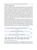
4. Sonar based localization
A challenge of mobile robot localization using sensor fusion is to weigh its pose (i.e. mobile
robot’s state) and sonar range reading (i.e. mobile robot’s output) uncertainties to get the op-
timal estimate of the pose, i.e. to minimize its covariance. The Kalman filter Kalman (1960)
assumes the Gaussian probability distributions of the state random variable such that it is
completely described with the mean and covariance. The optimal state estimate is computed
in two major stages: time-update and measurement-update. In the time-update, state pre-
diction is computed on the base of its preceding value and the control input value using the
motion model. Measurement-update uses the results from time-update to compute the out-
put predictions with the measurement model. Then the predicted state mean and covariance
are corrected in the sense of minimizing the state covariance with the weighted difference
between predicted and measured outputs. In succession, motion and measurement models
needed for the mobile robot sensor fusion are discussed, and then EKF and UKF algorithms
for mobile robot pose tracking are presented. Block diagram of implemented Kalman filter
based localization is given in Fig. 8.

non-linear
Kalman Filter
Measured wheel
speeds
Real sonar
measurements
Selection of
reliable sonar
measurements
reliable sonar
measurements
mobile robot pose
(state) prediction
Motion
model
Measurement
model
World model
(occupancy grid map)
Sonar
measurement
prediction
Fig. 8. Block diagram of non-linear Kalman filter localization approaches.
4.1 Occupancy grid world model
In mobile robotics, an occupancy grid is a two dimensional tessellation of the environment
map into a grid of equal or unequal cells. Each cell represents a modelled environment part
and holds information about the occupancy status of represented environment part. Occu-
pancy information can be of probabilistic or evidential nature and is often in the numeric
range from 0 to 1. Occupancy values closer to 0 mean that this environment part is free,
and occupancy values closer to 1 mean that an obstacle occupies this environment part. Val-

ues close to 0.5 mean that this particular environment part is not yet modelled and so its
occupancy value is unknown. When an exploration algorithm is used, this value is also an
indication that the mobile robot has not yet visited such environment parts. Some mapping
methods use this value as initial value. Figure 9 presents an example of ideal occupancy
grid map of a small environment. Left part of Fig. 9 presents outer walls of the environment
and cells belonging to an empty occupancy grid map (occupancy value of all cells set to
0 and filled with white color). Cells that overlap with environment walls should be filled
with information that this environment part is occupied (occupancy value set to 1 and filled
with black color as it can be seen in the right part of Fig. 9). It can be noticed that cells
make a discretization of the environment, so smaller cells are better for a more accurate map.
Drawback of smaller cells usage is increased memory consumption and decreased mapping
speed because occupancy information in more cells has to be updated during the mapping
process. A reasonable tradeoff between memory consumption, mapping speed, and map
accuracy can be made with cell size of 10 [cm] x 10 [cm]. Such a cell size is very common
when occupancy grid maps are used and is used in our research too.
ModelbasedKalmanFilterMobileRobotSelf-Localization 71
Robot
detection
mark
Robot pose
measuring
mark
Fig. 7. Mobile robot patch used for pose measurements
3.2 Camera calibration
Camera calibration in the context of threedimensional (3D) machine vision is the process of
determining the internal camera geometric and optical characteristics (intrinsic parameters)
or the 3D position and orientation of the camera frame relative to a certain world coordi-
nate system (extrinsic parameters) based on a number of points whose object coordinates in
the world coordinate system (X
i

, i = 1, 2, ··· , N) are known and whose image coordinates
(x
i
, i = 1, 2, ··· , N) are measured. It is a nonlinear optimization problem (20) whose solu-
tion is beyond the scope of this chapter. In our work perspective camera’s parameters were
determined by off-line camera calibration procedure described in Tsai (1987).
min
N
∑
i=1

SC
−1
X
i
− x
i

2
(20)
By this method with non-coplanar calibration target and full optimization, obtained were
the following intrinsic parameters for SONY EVI-D31 pan-tilt-zoom analog camera and
framegrabber with image resolution 320x240:
α
x
= α
y
= 379 [pixel],
x
0

= 165.9 [pixel], y
0
= 140 [pixel].
4. Sonar based localization
A challenge of mobile robot localization using sensor fusion is to weigh its pose (i.e. mobile
robot’s state) and sonar range reading (i.e. mobile robot’s output) uncertainties to get the op-
timal estimate of the pose, i.e. to minimize its covariance. The Kalman filter Kalman (1960)
assumes the Gaussian probability distributions of the state random variable such that it is
completely described with the mean and covariance. The optimal state estimate is computed
in two major stages: time-update and measurement-update. In the time-update, state pre-
diction is computed on the base of its preceding value and the control input value using the
motion model. Measurement-update uses the results from time-update to compute the out-
put predictions with the measurement model. Then the predicted state mean and covariance
are corrected in the sense of minimizing the state covariance with the weighted difference
between predicted and measured outputs. In succession, motion and measurement models
needed for the mobile robot sensor fusion are discussed, and then EKF and UKF algorithms
for mobile robot pose tracking are presented. Block diagram of implemented Kalman filter
based localization is given in Fig. 8.
non-linear
Kalman Filter
Measured wheel
speeds
Real sonar
measurements
Selection of
reliable sonar
measurements
reliable sonar
measurements
mobile robot pose

(state) prediction
Motion
model
Measurement
model
World model
(occupancy grid map)
Sonar
measurement
prediction
Fig. 8. Block diagram of non-linear Kalman filter localization approaches.
4.1 Occupancy grid world model
In mobile robotics, an occupancy grid is a two dimensional tessellation of the environment
map into a grid of equal or unequal cells. Each cell represents a modelled environment part
and holds information about the occupancy status of represented environment part. Occu-
pancy information can be of probabilistic or evidential nature and is often in the numeric
range from 0 to 1. Occupancy values closer to 0 mean that this environment part is free,
and occupancy values closer to 1 mean that an obstacle occupies this environment part. Val-
ues close to 0.5 mean that this particular environment part is not yet modelled and so its
occupancy value is unknown. When an exploration algorithm is used, this value is also an
indication that the mobile robot has not yet visited such environment parts. Some mapping
methods use this value as initial value. Figure 9 presents an example of ideal occupancy
grid map of a small environment. Left part of Fig. 9 presents outer walls of the environment
and cells belonging to an empty occupancy grid map (occupancy value of all cells set to
0 and filled with white color). Cells that overlap with environment walls should be filled
with information that this environment part is occupied (occupancy value set to 1 and filled
with black color as it can be seen in the right part of Fig. 9). It can be noticed that cells
make a discretization of the environment, so smaller cells are better for a more accurate map.
Drawback of smaller cells usage is increased memory consumption and decreased mapping
speed because occupancy information in more cells has to be updated during the mapping

process. A reasonable tradeoff between memory consumption, mapping speed, and map
accuracy can be made with cell size of 10 [cm] x 10 [cm]. Such a cell size is very common
when occupancy grid maps are used and is used in our research too.
RobotLocalizationandMapBuilding72
Fig. 9. Example of occupancy grid map environment
Obtained occupancy grid map given in the right part of Fig. 9 does not contain any unknown
space. A map generated using real sonar range measurement will contain some unknown
space, meaning that the whole environment has not been explored or that during exploration
no sonar range measurement defined the occupancy status of some environment part.
In order to use Kalman filter framework given in Fig. 8 for mobile robot pose estimation,
prediction of sonar sensor measurements has to be done. The sonar feature that most precise
measurement information is concentrated in the main axis of the sonar main lobe is used for
this step. So range measurement prediction is done using one propagated beam combined
with known local sensor coordinates and estimated mobile robot global pose. Measurement
prediction principle is depicted in Fig. 10.
Obstacle
Global coordinate
system center
Measured
range
Local coordinate
system center
Mobile robot
global position
Mobile robot
orientation
Sonar sensor
orientation
Sonar sensor angle
and range offset

Y
G
X
G
Y
L
X
L
Fig. 10. Sonar measurement prediction principle.
It has to be noticed that there are two sets of coordinates when measurement prediction is
done. Local coordinates defined to local coordinate system (its axis are denoted with X
L
and
Y
L
in Fig. 10) that is positioned in the axle center of the robot drive wheels. It moves with
the robot and its x-axis is always directed into the current robot motion direction. Sensors
coordinates are defined in this coordinate system and have to be transformed in the global
coordinate system center (its axis are denoted with X
G
and Y
G
in Fig. 10) to compute relative
distance between the sonar sensor and obstacles. This transformation for a particular sonar
sensor is given by the following equations:
S
XG
= x + S
o f f D
·cos


S
o f f Θ
+ Θ

, (21)
S
YG
= y + S
o f f D
·sin

S
o f f Θ
+ Θ

, (22)
S
ΘG
= Θ + S
sensΘ
, (23)
where coordinates x and y present mobile robot global position
[mm], Θ mobile robot global
orientation [
◦
], coordinates S
XG
and S
YG

sonar sensor position in global coordinates [mm],
S
ΘG
sonar sensor orientation in the global coordinate system frame [
◦
], S
o f f D
sonar sensor
distance from the center of the local coordinate system
[mm], S
o f f Θ
sonar sensor angular
offset towards local coordinate system [
◦
], and S
ΘG
sonar sensor orientation towards the
global coordinate system [
◦
].
After above described coordinate transformation is done, start point and direction of the
sonar acoustic beam are known. Center of the sound beam is propagated from the start
point until it hits an obstacle. Obtained beam length is then equal to predicted sonar range
measurement. Whence only sonar range measurements smaller or equal then 3.0 m are used,
measurements with a predicted value greater then 3.0 m are are being discarded. Greater
distances have a bigger possibility to originate from outliers and are so not good for pose
correction.
4.2 EKF localization
The motion model represents the way in which the current state follows from the previous
one. State vector is expressed as the mobile robot pose, x

k
=
[
x
k
y
k
Θ
k
]
T
, with respect to a
global coordinate frame, where k denotes the sampling instant. Its distribution is assumed
to be Gaussian, such that the state random variable is completely determined with a 3
×
3 covariance matrix P
k
and the state expectation (mean, estimate are used as synonyms).
Control input, u
k
, represents the commands to the robot to move from time step k to k + 1.
In the motion model u
k
=
[
D
k
∆Θ
k
]

T
represents translation for distance D
k
followed by a
rotation for angle ∆Θ
k
. The state transition function f(·) uses the state vector at the current
time instant and the current control input to compute the state vector at the next time instant:
x
k+1
= f(x
k
, u
k
, v
k
), (24)
where v
k
=

v
1,k
v
2,k

T
represents unpredictable process noise, that is assumed to be Gaus-
sian with zero mean, (E
{v

k
} = [0 0]
T
), and covariance Q
k
. With E {·} expectation function
is denoted. Using (1) to (3) the state transition function becomes:
f
(x
k
, u
k
, v
k
) =


x
k
+ (D
k
+ v
1,k
) · cos(Θ
k
+ ∆Θ
k
+ v
2,k
)

y
k
+ (D
k
+ v
1,k
) · sin(Θ
k
+ ∆Θ
k
+ v
2,k
)
Θ
k
+ ∆Θ
k
+ v
2,k


. (25)
The process noise covariance Q
k
was modelled on the assumption of two independent
sources of error, translational and angular, i.e. D
k
and ∆Θ
k
are added with corresponding

uncertainties. The expression for Q
k
is:
ModelbasedKalmanFilterMobileRobotSelf-Localization 73
Fig. 9. Example of occupancy grid map environment
Obtained occupancy grid map given in the right part of Fig. 9 does not contain any unknown
space. A map generated using real sonar range measurement will contain some unknown
space, meaning that the whole environment has not been explored or that during exploration
no sonar range measurement defined the occupancy status of some environment part.
In order to use Kalman filter framework given in Fig. 8 for mobile robot pose estimation,
prediction of sonar sensor measurements has to be done. The sonar feature that most precise
measurement information is concentrated in the main axis of the sonar main lobe is used for
this step. So range measurement prediction is done using one propagated beam combined
with known local sensor coordinates and estimated mobile robot global pose. Measurement
prediction principle is depicted in Fig. 10.
Obstacle
Global coordinate
system center
Measured
range
Local coordinate
system center
Mobile robot
global position
Mobile robot
orientation
Sonar sensor
orientation
Sonar sensor angle
and range offset

Y
G
X
G
Y
L
X
L
Fig. 10. Sonar measurement prediction principle.
It has to be noticed that there are two sets of coordinates when measurement prediction is
done. Local coordinates defined to local coordinate system (its axis are denoted with X
L
and
Y
L
in Fig. 10) that is positioned in the axle center of the robot drive wheels. It moves with
the robot and its x-axis is always directed into the current robot motion direction. Sensors
coordinates are defined in this coordinate system and have to be transformed in the global
coordinate system center (its axis are denoted with X
G
and Y
G
in Fig. 10) to compute relative
distance between the sonar sensor and obstacles. This transformation for a particular sonar
sensor is given by the following equations:
S
XG
= x + S
o f f D
·cos


S
o f f Θ
+ Θ

, (21)
S
YG
= y + S
o f f D
·sin

S
o f f Θ
+ Θ

, (22)
S
ΘG
= Θ + S
sensΘ
, (23)
where coordinates x and y present mobile robot global position
[mm], Θ mobile robot global
orientation [
◦
], coordinates S
XG
and S
YG

sonar sensor position in global coordinates [mm],
S
ΘG
sonar sensor orientation in the global coordinate system frame [
◦
], S
o f f D
sonar sensor
distance from the center of the local coordinate system
[mm], S
o f f Θ
sonar sensor angular
offset towards local coordinate system [
◦
], and S
ΘG
sonar sensor orientation towards the
global coordinate system [
◦
].
After above described coordinate transformation is done, start point and direction of the
sonar acoustic beam are known. Center of the sound beam is propagated from the start
point until it hits an obstacle. Obtained beam length is then equal to predicted sonar range
measurement. Whence only sonar range measurements smaller or equal then 3.0 m are used,
measurements with a predicted value greater then 3.0 m are are being discarded. Greater
distances have a bigger possibility to originate from outliers and are so not good for pose
correction.
4.2 EKF localization
The motion model represents the way in which the current state follows from the previous
one. State vector is expressed as the mobile robot pose, x

k
=
[
x
k
y
k
Θ
k
]
T
, with respect to a
global coordinate frame, where k denotes the sampling instant. Its distribution is assumed
to be Gaussian, such that the state random variable is completely determined with a 3
×
3 covariance matrix P
k
and the state expectation (mean, estimate are used as synonyms).
Control input, u
k
, represents the commands to the robot to move from time step k to k + 1.
In the motion model u
k
=
[
D
k
∆Θ
k
]

T
represents translation for distance D
k
followed by a
rotation for angle ∆Θ
k
. The state transition function f(·) uses the state vector at the current
time instant and the current control input to compute the state vector at the next time instant:
x
k+1
= f(x
k
, u
k
, v
k
), (24)
where v
k
=

v
1,k
v
2,k

T
represents unpredictable process noise, that is assumed to be Gaus-
sian with zero mean, (E
{v

k
} = [0 0]
T
), and covariance Q
k
. With E {·} expectation function
is denoted. Using (1) to (3) the state transition function becomes:
f
(x
k
, u
k
, v
k
) =


x
k
+ (D
k
+ v
1,k
) · cos(Θ
k
+ ∆Θ
k
+ v
2,k
)

y
k
+ (D
k
+ v
1,k
) · sin(Θ
k
+ ∆Θ
k
+ v
2,k
)
Θ
k
+ ∆Θ
k
+ v
2,k


. (25)
The process noise covariance Q
k
was modelled on the assumption of two independent
sources of error, translational and angular, i.e. D
k
and ∆Θ
k
are added with corresponding

uncertainties. The expression for Q
k
is:
RobotLocalizationandMapBuilding74
Q
k
=

σ
2
D
0
0 ∆Θ
2
k
σ
2
∆Θ

, (26)
where σ
2
D
and σ
2
∆Θ
are variances of D
k
and ∆Θ
k

, respectively.
The measurement model computes the range between an obstacle and the axle center of the
robot according to a measurement function Lee (1996):
h
i
(x, p
i
) =

(x
i
− x)
2
+ (y
i
−y)
2
, (27)
where p
i
= (x
i
, y
i
) denotes the point (occupied cell) in the world model detected by the ith
sonar. The sonar model uses (27) to relate a range reading to the obstacle that caused it:
z
i,k
= h
i

(x
k
, p
i
) + w
i,k
, (28)
where w
i,k
represents the measurement noise (Gaussian with zero mean and variance r
i,k
) for
the ith range reading. All range readings are used in parallel, such that range measurements
z
i,k
are simply stacked into a single measurement vector z
k
. Measurement covariance matrix
R
k
is a diagonal matrix with the elements r
i,k
. It is to be noted that the measurement noise is
additive, which will be beneficial for UKF implementation.
EKF is the first sensor fusion based mobile robot pose tracking technique presented in this
paper. Detailed explanation of used EKF localization can be found in Ivanjko et al. (2004)
and in the sequel only basic equations are presented. Values of the control input vector u
k−1
computed from wheels’ encoder data are passed to the algorithm at time k such that first
time-update is performed obtaining the prediction estimates, and then if new sonar readings

are available those predictions are corrected. Predicted (prior) state mean ˆx
−
k
is computed
in single-shot by propagating the state estimated at instant k
− 1, ˆx
k−1
through the true
nonlinear odometry mapping:
ˆx
−
k
= f( ˆx
k−1
, u
k−1
, E{v
k−1
}). (29)
The covariance of the predicted state P
−
k
is approximated with the covariance of the state
propagated through a linearized system from (24):
P
−
k
= ∇f
x
P

k−1
∇f
T
x
+ ∇f
u
Q
k
∇f
T
u
, (30)
where
∇f
x
= ∇f
x
(ˆx
k−1
, u
k−1
, E{v
k−1
}) is the Jacobian matrix of f with respect to x, while
∇f
u
= ∇f
u
(ˆx
k−1

, u
k−1
, E{v
k−1
}) is the Jacobian matrix of f(·) with respect to control input
u. It is to be noticed that using (29) and (30) the mean and covariance are accurate only to the
first-order of the corresponding Taylor series expansion Haykin (2001). If there are no new
sonar readings at instant k or if they are all rejected, measurement update does not occur
and the estimate mean and covariance are assigned with the predicted ones:
ˆx
k
= ˆx
−
k
, (31)
P
k
= P
−
k
. (32)
Otherwise, measurement-update takes place where first predictions of the accepted sonar
readings are collected in ˆz
−
k
with ith component of it being:
ˆ
z
−
i,k

= h
i
(ˆx
−
k
, p
i
) + E{w
i,k
}. (33)
The state estimate and its covariance in time step k are computed as follows:
ˆx
k
= ˆx
−
k
+ K
k
(z
k
− ˆz
−
k
), (34)
P
k
= (I −K
k
∇h
x

)P
−
k
, (35)
where z
k
are real sonar readings, ∇h
x
= ∇h
x
(ˆx
−
k
, E{w
k
}) is the Jacobian matrix of the
measurement function with respect to the predicted state, and K
k
is the optimal Kalman
gain computed as follows:
K
k
= P
−
k
∇h
T
x
(∇h
x

P
−
k
∇h
T
x
+ R
k
)
−1
. (36)
4.3 UKF localization
The second sensor fusion based mobile robot pose tracking technique presented in this chap-
ter uses UKF. UKF was first proposed by Julier et al. Julier & Uhlmann (1996), and further
developed by Wan and van der Merwe Haykin (2001). It utilizes the unscented transforma-
tion Julier & Uhlmann (1996) that approximates the true mean and covariance of a Gaussian
random variable propagated through nonlinear mapping accurate to the inclusively third
order of Taylor series expansion for any mapping. Following this, UKF approximates state
and output mean and covariance more accurately than EKF and thus superior operation of
UKF compared to EKF is expected. UKF was already used for mobile robot localization
in Ashokaraj et al. (2004) to fuse several sources of observations, and the estimates were,
if necessary, corrected using interval analysis on sonar measurements. Here we use sonar
measurements within UKF, without any other sensors except the encoders to capture angular
velocities of the drive wheels (motion model inputs), and without any additional estimate
corrections.
Means and covariances are in UKF case computed by propagating carefully chosen so called
pre-sigma points through the true nonlinear mapping. Nonlinear state-update with non-
additive Gaussian process noises in translation D and rotation ∆Θ is given in (25). The
measurement noise is additive and assumed to be Gaussian, see (28).
The UKF algorithm is initialized (k

= 0) with ˆx
0
and P
0
, same as the EKF. In case of non-
additive process noise and additive measurement noise, state estimate vector is augmented
with means of process noise E
{v
k−1
} only, thus forming extended state vector ˆx
a
k
−1
:
ˆx
a
k
−1
= E[x
a
k
−1
] =

ˆx
T
k
−1
E{v
k−1

}
T

T
. (37)
Measurement noise does not have to enter the ˆx
a
k
−1
because of additive properties Haykin
(2001). This is very important from implementation point of view since the dimension of out-
put is not known in advance because number of accepted sonar readings varies. Covariance
matrix is augmented accordingly forming matrix P
a
k
−1
:
P
a
k
−1
=

P
k−1
0
0 Q
k−1

. (38)

Time-update algorithm in time instant k first requires square root of the P
a
k
−1
(or lower
triangular Cholesky factorization),

P
a
k
−1
. Obtained lower triangular matrix is scaled by the
factor γ:
γ
=
√
L + λ, (39)
ModelbasedKalmanFilterMobileRobotSelf-Localization 75
Q
k
=

σ
2
D
0
0 ∆Θ
2
k
σ

2
∆Θ

, (26)
where σ
2
D
and σ
2
∆Θ
are variances of D
k
and ∆Θ
k
, respectively.
The measurement model computes the range between an obstacle and the axle center of the
robot according to a measurement function Lee (1996):
h
i
(x, p
i
) =

(x
i
− x)
2
+ (y
i
−y)

2
, (27)
where p
i
= (x
i
, y
i
) denotes the point (occupied cell) in the world model detected by the ith
sonar. The sonar model uses (27) to relate a range reading to the obstacle that caused it:
z
i,k
= h
i
(x
k
, p
i
) + w
i,k
, (28)
where w
i,k
represents the measurement noise (Gaussian with zero mean and variance r
i,k
) for
the ith range reading. All range readings are used in parallel, such that range measurements
z
i,k
are simply stacked into a single measurement vector z

k
. Measurement covariance matrix
R
k
is a diagonal matrix with the elements r
i,k
. It is to be noted that the measurement noise is
additive, which will be beneficial for UKF implementation.
EKF is the first sensor fusion based mobile robot pose tracking technique presented in this
paper. Detailed explanation of used EKF localization can be found in Ivanjko et al. (2004)
and in the sequel only basic equations are presented. Values of the control input vector u
k−1
computed from wheels’ encoder data are passed to the algorithm at time k such that first
time-update is performed obtaining the prediction estimates, and then if new sonar readings
are available those predictions are corrected. Predicted (prior) state mean ˆx
−
k
is computed
in single-shot by propagating the state estimated at instant k
− 1, ˆx
k−1
through the true
nonlinear odometry mapping:
ˆx
−
k
= f( ˆx
k−1
, u
k−1

, E{v
k−1
}). (29)
The covariance of the predicted state P
−
k
is approximated with the covariance of the state
propagated through a linearized system from (24):
P
−
k
= ∇f
x
P
k−1
∇f
T
x
+ ∇f
u
Q
k
∇f
T
u
, (30)
where
∇f
x
= ∇f

x
(ˆx
k−1
, u
k−1
, E{v
k−1
}) is the Jacobian matrix of f with respect to x, while
∇f
u
= ∇f
u
(ˆx
k−1
, u
k−1
, E{v
k−1
}) is the Jacobian matrix of f(·) with respect to control input
u. It is to be noticed that using (29) and (30) the mean and covariance are accurate only to the
first-order of the corresponding Taylor series expansion Haykin (2001). If there are no new
sonar readings at instant k or if they are all rejected, measurement update does not occur
and the estimate mean and covariance are assigned with the predicted ones:
ˆx
k
= ˆx
−
k
, (31)
P

k
= P
−
k
. (32)
Otherwise, measurement-update takes place where first predictions of the accepted sonar
readings are collected in ˆz
−
k
with ith component of it being:
ˆ
z
−
i,k
= h
i
(ˆx
−
k
, p
i
) + E{w
i,k
}. (33)
The state estimate and its covariance in time step k are computed as follows:
ˆx
k
= ˆx
−
k

+ K
k
(z
k
− ˆz
−
k
), (34)
P
k
= (I −K
k
∇h
x
)P
−
k
, (35)
where z
k
are real sonar readings, ∇h
x
= ∇h
x
(ˆx
−
k
, E{w
k
}) is the Jacobian matrix of the

measurement function with respect to the predicted state, and K
k
is the optimal Kalman
gain computed as follows:
K
k
= P
−
k
∇h
T
x
(∇h
x
P
−
k
∇h
T
x
+ R
k
)
−1
. (36)
4.3 UKF localization
The second sensor fusion based mobile robot pose tracking technique presented in this chap-
ter uses UKF. UKF was first proposed by Julier et al. Julier & Uhlmann (1996), and further
developed by Wan and van der Merwe Haykin (2001). It utilizes the unscented transforma-
tion Julier & Uhlmann (1996) that approximates the true mean and covariance of a Gaussian

random variable propagated through nonlinear mapping accurate to the inclusively third
order of Taylor series expansion for any mapping. Following this, UKF approximates state
and output mean and covariance more accurately than EKF and thus superior operation of
UKF compared to EKF is expected. UKF was already used for mobile robot localization
in Ashokaraj et al. (2004) to fuse several sources of observations, and the estimates were,
if necessary, corrected using interval analysis on sonar measurements. Here we use sonar
measurements within UKF, without any other sensors except the encoders to capture angular
velocities of the drive wheels (motion model inputs), and without any additional estimate
corrections.
Means and covariances are in UKF case computed by propagating carefully chosen so called
pre-sigma points through the true nonlinear mapping. Nonlinear state-update with non-
additive Gaussian process noises in translation D and rotation ∆Θ is given in (25). The
measurement noise is additive and assumed to be Gaussian, see (28).
The UKF algorithm is initialized (k
= 0) with ˆx
0
and P
0
, same as the EKF. In case of non-
additive process noise and additive measurement noise, state estimate vector is augmented
with means of process noise E
{v
k−1
} only, thus forming extended state vector ˆx
a
k
−1
:
ˆx
a

k
−1
= E[x
a
k
−1
] =

ˆx
T
k
−1
E{v
k−1
}
T

T
. (37)
Measurement noise does not have to enter the ˆx
a
k
−1
because of additive properties Haykin
(2001). This is very important from implementation point of view since the dimension of out-
put is not known in advance because number of accepted sonar readings varies. Covariance
matrix is augmented accordingly forming matrix P
a
k
−1

:
P
a
k
−1
=

P
k−1
0
0 Q
k−1

. (38)
Time-update algorithm in time instant k first requires square root of the P
a
k
−1
(or lower
triangular Cholesky factorization),

P
a
k
−1
. Obtained lower triangular matrix is scaled by the
factor γ:
γ
=
√

L + λ, (39)
RobotLocalizationandMapBuilding76
where L represents the dimension of augmented state x
a
k
−1
(L = 5 in this application), and λ
is a scaling parameter computed as follows:
λ
= α
2
(L + κ) − L. (40)
Parameter α can be chosen within range
[10
−4
, 1], and κ is usually set to 1. There are 2L + 1
pre-sigma points, the first is ˆx
a
k
−1
itself, and other 2L are obtained by adding to or subtracting
from ˆx
a
k
−1
each of L columns of γ

P
a
k

−1
, symbolically written as:
X
a
k
−1
=

ˆx
a
k
−1
ˆx
a
k
−1
+ γ

P
a
k
−1
ˆx
a
k
−1
−γ

P
a

k
−1

, (41)
where
X
a
k
−1
= [(X
x
k
−1
)
T
(X
v
k
−1
)
T
]
T
represents the matrix whose columns are pre-sigma
points. All pre-sigma points are processed by the state-update function obtaining matrix
X
x
k
|k−1
of predicted states for each pre-sigma point, symbolically written as:

X
x
k
|k−1
= f[X
x
k
−1
, u
k−1
, X
v
k
−1
]. (42)
Prior mean is calculated as weighted sum of acquired points:
ˆx
−
k
=
2L
∑
i=0
W
(m)
i
X
x
i,k
|k−1

, (43)
where
X
x
i,k
|k−1
denotes the ith column of X
x
k
|k−1
. Weights for mean calculation W
(m)
i
are given
by
W
(m)
0
=
λ
L + λ
, (44)
W
(m)
i
=
1
2(L + λ)
, i = 1, . . . , 2L. (45)
Prior covariance matrix P

−
k
is given by
P
−
k
=
2L
∑
i=0
W
(c)
i
[X
x
i,k
|k−1
− ˆx
−
k
][X
x
i,k
|k−1
− ˆx
−
k
]
T
, (46)

where W
(c)
i
represent the weights for covariance calculation which are given by
W
(c)
0
=
λ
L + λ
+ (1 − α
2
+ β), (47)
W
(c)
i
=
1
2(L + λ)
, i = 1, . . . , 2L. (48)
For Gaussian distributions β
= 2 is optimal.
If there are new sonar readings available at time instant k, predicted readings of accepted
sonars for each sigma-point are grouped in matrix
Z
k|k−1
obtained by
Z
k|k−1
= h[X

x
k
|k−1
, p] + E{w
k
}, (49)
where p denotes the series of points in the world map predicted to be hit by sonar beams.
Predicted readings ˆz
−
k
are then
ˆz
−
k
=
2L
∑
i=0
W
(m)
i
Z
i,k|k−1
. (50)
To prevent the sonar readings that hit near the corner of obstacles to influence on the mea-
surement correction, since their probability distribution cannot be approximated with Gaus-
sian, another threshold comparison were made. These problematic sonar readings are recog-
nized with mean
ˆ
z

−
i,k
that differs from z
i,k
more than the acceptation threshold amounts, and
those are being discarded. Readings covariance is
P
z
k
=
2L
∑
i=0
W
(c)
i
[Z
i,k|k−1
− ˆz
−
k
][Z
i,k|k−1
− ˆz
−
k
]
T
+ R
k

, (51)
and state-output cross-covariance matrix is
P
x
k
z
k
=
2L
∑
i=0
W
(c)
i
[X
x
i,k
|k−1
− ˆx
−
k
][Z
i,k|k−1
− ˆz
−
k
]
T
. (52)
Kalman gain K

k
is
K
k
= P
x
k
z
k
P
−1
z
k
. (53)
Posterior state covariance is finally calculated as
P
k
= P
−
k
−K
k
P
z
k
K
T
k
. (54)
The measurement correction is done as in (34).

5. Monocular vision based localization
In this section, we consider the problem of mobile robot pose estimation using only visual
information from a single camera and odometry readings. Focus is on building complex
environmental models, fast online rendering and real-time complex and noisy image seg-
mentation. The 3D model of the mobile robot’s environment is built using a professional
freeware computer graphics tool named Blender and pre-stored in the memory of the robot’s
on-board computer. Estimation of the mobile robot pose as a stochastic variable is done
by correspondences of image lines, extracted using Random Window Randomized Hough
Transform line detection algorithm, and model lines, predicted using odometry readings
and 3D environment model. The camera model and ray tracing algorithm are also described.
Developed algorithms are also experimentally tested using a Pioneer 2DX mobile robot.
5.1 Scene modelling and rendering
Referential model of the environment was built using Blender, where vertices, edges (lines)
and faces (planes) were used for model notation. An edge is defined with two vertices and a
face with three or four vertices. The drawn model is one object in which all vertices, edges
and faces are listed. For illustration, in Fig. 11, 3D model of the hallway in which our mobile
robot moves is shown. Although the environment model is quite complex, we achieved
online execution of the localization algorithms by applying fast rendering. Namely, in each
ModelbasedKalmanFilterMobileRobotSelf-Localization 77
where L represents the dimension of augmented state x
a
k
−1
(L = 5 in this application), and λ
is a scaling parameter computed as follows:
λ
= α
2
(L + κ) − L. (40)
Parameter α can be chosen within range

[10
−4
, 1], and κ is usually set to 1. There are 2L + 1
pre-sigma points, the first is ˆx
a
k
−1
itself, and other 2L are obtained by adding to or subtracting
from ˆx
a
k
−1
each of L columns of γ

P
a
k
−1
, symbolically written as:
X
a
k
−1
=

ˆx
a
k
−1
ˆx

a
k
−1
+ γ

P
a
k
−1
ˆx
a
k
−1
−γ

P
a
k
−1

, (41)
where
X
a
k
−1
= [(X
x
k
−1

)
T
(X
v
k
−1
)
T
]
T
represents the matrix whose columns are pre-sigma
points. All pre-sigma points are processed by the state-update function obtaining matrix
X
x
k
|k−1
of predicted states for each pre-sigma point, symbolically written as:
X
x
k
|k−1
= f[X
x
k
−1
, u
k−1
, X
v
k

−1
]. (42)
Prior mean is calculated as weighted sum of acquired points:
ˆx
−
k
=
2L
∑
i=0
W
(m)
i
X
x
i,k
|k−1
, (43)
where
X
x
i,k
|k−1
denotes the ith column of X
x
k
|k−1
. Weights for mean calculation W
(m)
i

are given
by
W
(m)
0
=
λ
L
+ λ
, (44)
W
(m)
i
=
1
2
(L + λ)
, i = 1, . . . , 2L. (45)
Prior covariance matrix P
−
k
is given by
P
−
k
=
2L
∑
i=0
W

(c)
i
[X
x
i,k
|k−1
− ˆx
−
k
][X
x
i,k
|k−1
− ˆx
−
k
]
T
, (46)
where W
(c)
i
represent the weights for covariance calculation which are given by
W
(c)
0
=
λ
L
+ λ

+ (1 − α
2
+ β), (47)
W
(c)
i
=
1
2
(L + λ)
, i = 1, . . . , 2L. (48)
For Gaussian distributions β
= 2 is optimal.
If there are new sonar readings available at time instant k, predicted readings of accepted
sonars for each sigma-point are grouped in matrix
Z
k|k−1
obtained by
Z
k|k−1
= h[X
x
k
|k−1
, p] + E{w
k
}, (49)
where p denotes the series of points in the world map predicted to be hit by sonar beams.
Predicted readings ˆz
−

k
are then
ˆz
−
k
=
2L
∑
i=0
W
(m)
i
Z
i,k|k−1
. (50)
To prevent the sonar readings that hit near the corner of obstacles to influence on the mea-
surement correction, since their probability distribution cannot be approximated with Gaus-
sian, another threshold comparison were made. These problematic sonar readings are recog-
nized with mean
ˆ
z
−
i,k
that differs from z
i,k
more than the acceptation threshold amounts, and
those are being discarded. Readings covariance is
P
z
k

=
2L
∑
i=0
W
(c)
i
[Z
i,k|k−1
− ˆz
−
k
][Z
i,k|k−1
− ˆz
−
k
]
T
+ R
k
, (51)
and state-output cross-covariance matrix is
P
x
k
z
k
=
2L

∑
i=0
W
(c)
i
[X
x
i,k
|k−1
− ˆx
−
k
][Z
i,k|k−1
− ˆz
−
k
]
T
. (52)
Kalman gain K
k
is
K
k
= P
x
k
z
k

P
−1
z
k
. (53)
Posterior state covariance is finally calculated as
P
k
= P
−
k
−K
k
P
z
k
K
T
k
. (54)
The measurement correction is done as in (34).
5. Monocular vision based localization
In this section, we consider the problem of mobile robot pose estimation using only visual
information from a single camera and odometry readings. Focus is on building complex
environmental models, fast online rendering and real-time complex and noisy image seg-
mentation. The 3D model of the mobile robot’s environment is built using a professional
freeware computer graphics tool named Blender and pre-stored in the memory of the robot’s
on-board computer. Estimation of the mobile robot pose as a stochastic variable is done
by correspondences of image lines, extracted using Random Window Randomized Hough
Transform line detection algorithm, and model lines, predicted using odometry readings

and 3D environment model. The camera model and ray tracing algorithm are also described.
Developed algorithms are also experimentally tested using a Pioneer 2DX mobile robot.
5.1 Scene modelling and rendering
Referential model of the environment was built using Blender, where vertices, edges (lines)
and faces (planes) were used for model notation. An edge is defined with two vertices and a
face with three or four vertices. The drawn model is one object in which all vertices, edges
and faces are listed. For illustration, in Fig. 11, 3D model of the hallway in which our mobile
robot moves is shown. Although the environment model is quite complex, we achieved
online execution of the localization algorithms by applying fast rendering. Namely, in each
RobotLocalizationandMapBuilding78
Fig. 11. Hallway 3D model
step we render only the small region enclosed with the camera frustrum and then apply a
ray tracing algorithm to solve the occlusion problems.
The above described notation of the scene model, enables us to implement a ray tracing
algorithm. The algorithm is organized in two ”for” loops, as shown in Fig. 12(b), where the
algorithm flowchart is depicted. The first (outer) loop goes over the edge list and the second
(inner) loop goes over the face list. The outer loop starts with the function IsInsideFrustrum
(point3D), which examines whether observed points are located inside the camera frustrum
and discards those that are not in it. Then, for a point p in the frustrum, where p is the point
in the middle of the edge determined with two vertices, e.vert1 and e.vert2, as shown in Fig.
12(a), the direction of the vector ray is defined with point p and camera pose (cam_pos).
The inner loop starts with choosing a plane f from the list of faces, and then the function
Intersect (f, vector) returns intersection point P
T
between the given plane f and direction
vector as an output value, or None if the intersection doesn’t exist. Visible edges are checked
by comparing distances from the camera pose to the the point p (dist1) and to intersection
point P
T
(dist2), see Fig. 12(a). If these two distances do not match, the checked model edge

(line) is invisible, and therefore not used in later matching procedure.
Notice the incompleteness of rendering because only edges whose middle point is visible
will be rendered visible. That does not affect the accuracy of the later matching algorithm
for partially visible model lines because it is done in Hough space where a line is represented
with a single point regarding its length. The rendering could produce only smaller number
of partially visible lines, but in this case it is not important because there are still enough
lines for estimating mobile robot’s pose while gaining faster algorithm execution.
5.2 Image segmentation
Mobile robot self-localization requires matching of edge segments in the current camera im-
age and edge segments in the environment model seen from the expected mobile robot pose.
In previous section we described line extraction from the environment model, and below
we describe the line extraction in the camera image (image segmentation). Image segmen-
tation is done by the Canny edge detector and RWRHT line detector algorithm described in
Kälviäinen et al. (1994). The RWRHT is based on Randomized Hough Transformation (RHT),
which selects n pixels from the edge image by random sampling to solve n parameters of
e.vert1
e.vert2
p(x,y,z)
cam_pos
T
1
T
2
T
3
T
4
T
T
T

T
5
7
8
6
dist2
dist1
X
Z
Y
trace
P
T
f
(a) model
for e in data.edges:
If [ IsInsideFrustrum(e.vert1) == True or
IsInsideFrustrum(e.vert2) == True or
IsInsideFrustrum(p) == True ]
ray = p - cam_pos
dist1 = || p – cam_pos ||
trace = None
foundVisible = 1
for f in data.fa ces:
trace = Intersect (f, ray)
if (trace != None)
If [ IsInsideFrustrum(trace) == Tru e ]
dist2 = || trace – cam_pos ||
If [ (dist1 – dist2) > eps ]
foundVisible = 0

If (foundVisible == 1)
write edge in file
End of ray
tracing
f reaches
the end of
data.faces
e reaches
the end of
data.edges
False
False
False
False
(b) algorithm flowchart
Fig. 12. Ray tracing
a curve, and then accumulates only one cell in parameter space. Detected curves are those
whose accumulator cell is greater then predefined threshold. The RWRHT is an extension of
the RHT on complex and noisy images that applies RHT to a limited neighborhood of edge
pixels. The benefit is the reduction of the computational power and memory resources. The
pseudo-code of the RWHT is written in Algorithm 2.
5.3 Mobile robot pose estimation
Once the correspondences have been established between image lines and model lines seen
from the current mobile robot pose, we could update the mobile robot pose by applying
an appropriate estimation technique. In most cases, linearized system and measurement
equations and Gaussian noise in states and measurements are satisfactory approximations.
Therefore, we apply Extended Kalman Filter (EKF) Welch & Bishop (2000), which is an opti-
mal estimator under the above assumptions.
The state vector that is to be estimated is the mobile robot pose p. Introducing uncertainty
in the equations (1), (2) and (3) as the zero mean Gaussian additive noise, the state equations

are obtained:
p
n+1
= f
[
p
n
, v(n), ω(n )
]
+ w(n), (55)
where w
∼ N(0, Q).
ModelbasedKalmanFilterMobileRobotSelf-Localization 79
Fig. 11. Hallway 3D model
step we render only the small region enclosed with the camera frustrum and then apply a
ray tracing algorithm to solve the occlusion problems.
The above described notation of the scene model, enables us to implement a ray tracing
algorithm. The algorithm is organized in two ”for” loops, as shown in Fig. 12(b), where the
algorithm flowchart is depicted. The first (outer) loop goes over the edge list and the second
(inner) loop goes over the face list. The outer loop starts with the function IsInsideFrustrum
(point3D), which examines whether observed points are located inside the camera frustrum
and discards those that are not in it. Then, for a point p in the frustrum, where p is the point
in the middle of the edge determined with two vertices, e.vert1 and e.vert2, as shown in Fig.
12(a), the direction of the vector ray is defined with point p and camera pose (cam_pos).
The inner loop starts with choosing a plane f from the list of faces, and then the function
Intersect (f, vector) returns intersection point P
T
between the given plane f and direction
vector as an output value, or None if the intersection doesn’t exist. Visible edges are checked
by comparing distances from the camera pose to the the point p (dist1) and to intersection

point P
T
(dist2), see Fig. 12(a). If these two distances do not match, the checked model edge
(line) is invisible, and therefore not used in later matching procedure.
Notice the incompleteness of rendering because only edges whose middle point is visible
will be rendered visible. That does not affect the accuracy of the later matching algorithm
for partially visible model lines because it is done in Hough space where a line is represented
with a single point regarding its length. The rendering could produce only smaller number
of partially visible lines, but in this case it is not important because there are still enough
lines for estimating mobile robot’s pose while gaining faster algorithm execution.
5.2 Image segmentation
Mobile robot self-localization requires matching of edge segments in the current camera im-
age and edge segments in the environment model seen from the expected mobile robot pose.
In previous section we described line extraction from the environment model, and below
we describe the line extraction in the camera image (image segmentation). Image segmen-
tation is done by the Canny edge detector and RWRHT line detector algorithm described in
Kälviäinen et al. (1994). The RWRHT is based on Randomized Hough Transformation (RHT),
which selects n pixels from the edge image by random sampling to solve n parameters of
e.vert1
e.vert2
p(x,y,z)
cam_pos
T
1
T
2
T
3
T
4

T
T
T
T
5
7
8
6
dist2
dist1
X
Z
Y
trace
P
T
f
(a) model
for e in data.edges:
If [ IsInsideFrustrum(e.vert1) == True or
IsInsideFrustrum(e.vert2) == True or
IsInsideFrustrum(p) == True ]
ray = p - cam_pos
dist1 = || p – cam_pos ||
trace = None
foundVisible = 1
for f in data.fa ces:
trace = Intersect (f, ray)
if (trace != None)
If [ IsInsideFrustrum(trace) == Tru e ]

dist2 = || trace – cam_pos ||
If [ (dist1 – dist2) > eps ]
foundVisible = 0
If (foundVisible == 1)
write edge in file
End of ray
tracing
f reaches
the end of
data.faces
e reaches
the end of
data.edges
False
False
False
False
(b) algorithm flowchart
Fig. 12. Ray tracing
a curve, and then accumulates only one cell in parameter space. Detected curves are those
whose accumulator cell is greater then predefined threshold. The RWRHT is an extension of
the RHT on complex and noisy images that applies RHT to a limited neighborhood of edge
pixels. The benefit is the reduction of the computational power and memory resources. The
pseudo-code of the RWHT is written in Algorithm 2.
5.3 Mobile robot pose estimation
Once the correspondences have been established between image lines and model lines seen
from the current mobile robot pose, we could update the mobile robot pose by applying
an appropriate estimation technique. In most cases, linearized system and measurement
equations and Gaussian noise in states and measurements are satisfactory approximations.
Therefore, we apply Extended Kalman Filter (EKF) Welch & Bishop (2000), which is an opti-

mal estimator under the above assumptions.
The state vector that is to be estimated is the mobile robot pose p. Introducing uncertainty
in the equations (1), (2) and (3) as the zero mean Gaussian additive noise, the state equations
are obtained:
p
n+1
= f
[
p
n
, v(n), ω(n )
]
+ w(n), (55)
where w
∼ N(0, Q).
RobotLocalizationandMapBuilding80
Algorithm 2 The Random Window RHT Algorithm
1: D ⇐ all edge points in binary edge picture
2: d
i
⇐ randomly selected point from set D
3: m ⇐ randomly selected window size where m
min
≤ m ≤ m
max
4: W ⇐ pixel data set of m × m neighborhood of the point d
i
5: repeat
6: RHT algorithm on the set W
7: until maximum R times

8: if accumulator cell ≥ threshold then
9: corresponding parameters are the parameters of detected curve
10: else
11: goto 2
12: end if
Measurement is a set S of pairs "model line - image line":
S = {{m, i}|m = visible model line,
i = image line - perspective projection of m
}.
(56)
The straight line in the world coordinate system which passes through the point (x
0
, y
0
, z
0
)
and has direction coefficients (a, b, c) is given by:


x
y
z


=


a
b

c


u
+


x
0
y
0
z
0


, u
∈ . (57)
The straight line in image plane is given by
x cosγ
+ y sinγ = ρ, ρ ≥ 0, γ ∈ [0, 2π], (58)
where ρ and γ are the Hough space parameters of the line.
Let by applying perspective projection transformation P to a 3D model line we obtain 2D
straight line m and let its pair line i in the image be defined with the Hough space parameters
(ρ, γ). The projection of the 3D point (x
0
, y
0
, z
0
) lies on the image line i and direction

coefficients of m and i lines are the same if the following conditions are fulfilled:
z
1
= W


ρ cosγ
ρ sinγ
1


− P




x
0
y
0
z
0
1




= 0, (59)
z
2

=


−sinγ
cosγ
0


−
P




a
b
c
0





















P




a
b
c
0





















= 0, (60)
z
=
[
z
1
, z
2
]

. (61)
Equations (59) and (60) are measurement equations and are used to correct mobile robot pose
with each correct match. Uncertainty in mobile robot pose means uncertainty in model lines
and is propagated to the Hough space in the same way as in Kosaka & Kak (1992), so we
will not go into details but only explain the main concept. For differentials of the equation
(15) we obtain
δX
=

δX
δY

= J

P
(M,
ˆ
p) δp , (62)
where J
P
(
ˆ
p
) is Jacobian of perspective projection of the end point of 3D model line M taken
at expected values of random vector p. Notice that from this point on, we are using first
order Taylor approximations of nonlinear transformations. Covariance matrix related to pixel
coordinates of a single model line point is given by:
Σ
X
= E[ δX δX

] = J
P
(M,
ˆ
p) Σ
p
J
P
(M,
ˆ
p)

, (63)

where Σ
p
is covariance matrix of mobile robot pose p. So, at this moment, we have deter-
mined uncertainty convex hull in which the probability of finding corresponding image line
is the highest. Furthermore, we can apply Hough transform
H to that line segment, which
would lead to point representation
ˆ
h
= (ρ, γ) of the line on which the segment coincides with
elliptical uncertainty region defined by the Mahalanobious distance and covariance matrix.
If J
H
denotes Jacobian of the Hough transform H with respect to variables ρ and γ we can
write:

δρ
δγ

= J
H




δX
1
δY
1
δX

2
δY
2




, (64)
Σ
ργ
= J
H

J
P
(M
1
, ˆp) 0
0 J
P
(M
2
, ˆp)

Σ
p

J
P
(M

1
, ˆp) 0
0 J
P
(M
2
, ˆp)


J

H
. (65)
ModelbasedKalmanFilterMobileRobotSelf-Localization 81
Algorithm 2 The Random Window RHT Algorithm
1: D ⇐ all edge points in binary edge picture
2: d
i
⇐ randomly selected point from set D
3: m ⇐ randomly selected window size where m
min
≤ m ≤ m
max
4: W ⇐ pixel data set of m × m neighborhood of the point d
i
5: repeat
6: RHT algorithm on the set W
7: until maximum R times
8: if accumulator cell ≥ threshold then
9: corresponding parameters are the parameters of detected curve

10: else
11: goto 2
12: end if
Measurement is a set
S of pairs "model line - image line":
S = {{m, i}|m = visible model line,
i = image line - perspective projection of m
}.
(56)
The straight line in the world coordinate system which passes through the point (x
0
, y
0
, z
0
)
and has direction coefficients (a, b, c) is given by:


x
y
z


=


a
b
c



u
+


x
0
y
0
z
0


, u
∈ . (57)
The straight line in image plane is given by
x cosγ
+ y sinγ = ρ, ρ ≥ 0, γ ∈ [0, 2π], (58)
where ρ and γ are the Hough space parameters of the line.
Let by applying perspective projection transformation P to a 3D model line we obtain 2D
straight line m and let its pair line i in the image be defined with the Hough space parameters
(ρ, γ). The projection of the 3D point (x
0
, y
0
, z
0
) lies on the image line i and direction
coefficients of m and i lines are the same if the following conditions are fulfilled:

z
1
= W


ρ cosγ
ρ sinγ
1


− P




x
0
y
0
z
0
1




= 0, (59)
z
2
=



−sinγ
cosγ
0


−
P




a
b
c
0





















P




a
b
c
0





















= 0, (60)
z
=
[
z
1
, z
2
]

. (61)
Equations (59) and (60) are measurement equations and are used to correct mobile robot pose
with each correct match. Uncertainty in mobile robot pose means uncertainty in model lines
and is propagated to the Hough space in the same way as in Kosaka & Kak (1992), so we
will not go into details but only explain the main concept. For differentials of the equation
(15) we obtain
δX
=

δX
δY

= J
P

(M,
ˆ
p) δp , (62)
where J
P
(
ˆ
p
) is Jacobian of perspective projection of the end point of 3D model line M taken
at expected values of random vector p. Notice that from this point on, we are using first
order Taylor approximations of nonlinear transformations. Covariance matrix related to pixel
coordinates of a single model line point is given by:
Σ
X
= E[ δX δX

] = J
P
(M,
ˆ
p) Σ
p
J
P
(M,
ˆ
p)

, (63)
where Σ

p
is covariance matrix of mobile robot pose p. So, at this moment, we have deter-
mined uncertainty convex hull in which the probability of finding corresponding image line
is the highest. Furthermore, we can apply Hough transform
H to that line segment, which
would lead to point representation
ˆ
h
= (ρ, γ) of the line on which the segment coincides with
elliptical uncertainty region defined by the Mahalanobious distance and covariance matrix.
If J
H
denotes Jacobian of the Hough transform H with respect to variables ρ and γ we can
write:

δρ
δγ

= J
H




δX
1
δY
1
δX
2

δY
2




, (64)
Σ
ργ
= J
H

J
P
(M
1
, ˆp) 0
0 J
P
(M
2
, ˆp)

Σ
p

J
P
(M
1

, ˆp) 0
0 J
P
(M
2
, ˆp)


J

H
. (65)
RobotLocalizationandMapBuilding82
We limit the search for image lines to uncertainty region in the Hough space ⊂ 
2
deter-
mined by the constraint:
(h −
ˆ
h
)Σ
−1
ργ
(h −
ˆ
h
)
T
≤ 2.
This rises a matching problem if one model line has more then one image candidate, but the

problem was solved in Kosaka & Kak (1992) and Aider et al. (2005).
There are also quantization error, noise in camera image and error in edge detection and
image segmentation which have been approximated by Gaussian variable ξ
∼ N(0, V) and
included in the EKF equations as the measurement noise. Finally, the equations of the im-
plemented EKF are:
a priori update:
ˆp
n+1
= f
[
ˆ
p
n
, v(n), ω(n )
]
, (66)
ˆz
n
= z

ˆp
n
,
ˆ
h(i)
i→m

, (67)
Σ

p
n+1 |n
= A Σ
p
n
A

+ Q, A = ∂f/∂p|
p=
ˆ
p
, (68)
a posteriori update:
K
n+1
= Σ
p
n+1 |n
H


H Σ
p
n+1 |n
H

+ R

, (69)
p

n+1
= ˆp
n+1
+ K
n+1
(z − ˆz
n
), (70)
Σ
p
n+1
= (I − K
n+1
H)Σ
p
n+1 |n
, (71)
where H
=
∂z
∂p
|
p=
ˆ
p
and R =
∂z
∂h
|
h=

ˆ
h
·V ·
∂z
∂h

|
h=
ˆ
h
.
6. Experimental results
This section presents obtained experimental results including description of experimental
setup and experiment conditions. First are presented results obtained using sonar sensors
and after that results obtained using monocular-vision. Section ends with comments on
obtained results.
6.1 Experimental setup description
Experiments are performed using a Pioneer 2DX mobile robot from MobileRobots. Its con-
figuration is presented in Fig. 13 only that in localization experiments monocular camera was
used insted of depicted stereo one. Used sensors are encoders for odometry, sonars, mono-
camera and a laser range finder. Laser range finder was used only for a comparison purpose
as a sensor that enables a more accurate localization than the sonars or mono-camera. It
is combined with a Monte-Carlo algorithm Konolige (1999) implemented as standard local-
ization solution in the mobile robot control software. Used camera for monocular-vision
localization is a SONY EVI-D31 pan-tilt-zoom analog camera. Laser sensor is a SICK LMS-
200, and sonars are Polaroid 6500 sensors.
Experimental environment including trajectory traversed by the mobile robot is presented in
Fig. 14. Global coordinate system is depicted on the left side. It’s a hallway with several door
niches. Mobile robot movement started in one corridor end and ended when it reached other
corridor end. Trajectory length is approximately 20 [m] and is generated using a gradient

based algorithm described in Konolige (2000). Obstacle avoidance was also active during all
experiments.
stereo-camera
on-board
computer
WLAN antenna
bumpers
LRF
sensor
sonars
RS232 interface for
piggy-back laptop
Fig. 13. Pioneer 2DX mobile robot
Fig. 14. Mobile robot trajectory for experimental evaluation.
Initial robot’s pose and its covariance was in all experiments set to (orientation given in
radians):
p
0
=

210 dm 9.25 dm π


,
Σ
p
0
=



0.3000 0 0
0 0.3000 0
0 0 0.0080


,
which means about 0.55
[
dm
]
standard deviation in p
x
and p
y
and about 5
[
◦
]
standard
deviation in robot orientation. In every experiment mobile robot start pose was manually set
according to marks on the hallway floor, so given initial pose covariance was set to cover start
pose setting error margins. Experiments show that implemented self-localization algorithms
were able to cope with that starting pose error margins.
During all experiments relevant measurements data were collected and saved for obtained lo-
calization quality evaluation. Saved data included mobile robot drive wheel speeds, sampling
period, sonar range measurements, camera images, evaluated self-localization algorithm es-
timated pose and Monte Carlo based localization results. Pose obtained using Monte Carlo
ModelbasedKalmanFilterMobileRobotSelf-Localization 83
We limit the search for image lines to uncertainty region in the Hough space ⊂ 
2

deter-
mined by the constraint:
(h −
ˆ
h
)Σ
−1
ργ
(h −
ˆ
h
)
T
≤ 2.
This rises a matching problem if one model line has more then one image candidate, but the
problem was solved in Kosaka & Kak (1992) and Aider et al. (2005).
There are also quantization error, noise in camera image and error in edge detection and
image segmentation which have been approximated by Gaussian variable ξ
∼ N(0, V) and
included in the EKF equations as the measurement noise. Finally, the equations of the im-
plemented EKF are:
a priori update:
ˆp
n+1
= f
[
ˆ
p
n
, v(n), ω(n )

]
, (66)
ˆz
n
= z

ˆp
n
,
ˆ
h(i)
i→m

, (67)
Σ
p
n+1 |n
= A Σ
p
n
A

+ Q, A = ∂f/∂p|
p=
ˆ
p
, (68)
a posteriori update:
K
n+1

= Σ
p
n+1 |n
H


H Σ
p
n+1 |n
H

+ R

, (69)
p
n+1
= ˆp
n+1
+ K
n+1
(z − ˆz
n
), (70)
Σ
p
n+1
= (I − K
n+1
H)Σ
p

n+1 |n
, (71)
where H
=
∂z
∂p
|
p=
ˆ
p
and R =
∂z
∂h
|
h=
ˆ
h
·V ·
∂z
∂h

|
h=
ˆ
h
.
6. Experimental results
This section presents obtained experimental results including description of experimental
setup and experiment conditions. First are presented results obtained using sonar sensors
and after that results obtained using monocular-vision. Section ends with comments on

obtained results.
6.1 Experimental setup description
Experiments are performed using a Pioneer 2DX mobile robot from MobileRobots. Its con-
figuration is presented in Fig. 13 only that in localization experiments monocular camera was
used insted of depicted stereo one. Used sensors are encoders for odometry, sonars, mono-
camera and a laser range finder. Laser range finder was used only for a comparison purpose
as a sensor that enables a more accurate localization than the sonars or mono-camera. It
is combined with a Monte-Carlo algorithm Konolige (1999) implemented as standard local-
ization solution in the mobile robot control software. Used camera for monocular-vision
localization is a SONY EVI-D31 pan-tilt-zoom analog camera. Laser sensor is a SICK LMS-
200, and sonars are Polaroid 6500 sensors.
Experimental environment including trajectory traversed by the mobile robot is presented in
Fig. 14. Global coordinate system is depicted on the left side. It’s a hallway with several door
niches. Mobile robot movement started in one corridor end and ended when it reached other
corridor end. Trajectory length is approximately 20 [m] and is generated using a gradient
based algorithm described in Konolige (2000). Obstacle avoidance was also active during all
experiments.
stereo-camera
on-board
computer
WLAN antenna
bumpers
LRF
sensor
sonars
RS232 interface for
piggy-back laptop
Fig. 13. Pioneer 2DX mobile robot
Fig. 14. Mobile robot trajectory for experimental evaluation.
Initial robot’s pose and its covariance was in all experiments set to (orientation given in

radians):
p
0
=

210 dm 9.25 dm π


,
Σ
p
0
=


0.3000 0 0
0 0.3000 0
0 0 0.0080


,
which means about 0.55
[
dm
]
standard deviation in p
x
and p
y
and about 5

[
◦
]
standard
deviation in robot orientation. In every experiment mobile robot start pose was manually set
according to marks on the hallway floor, so given initial pose covariance was set to cover start
pose setting error margins. Experiments show that implemented self-localization algorithms
were able to cope with that starting pose error margins.
During all experiments relevant measurements data were collected and saved for obtained lo-
calization quality evaluation. Saved data included mobile robot drive wheel speeds, sampling
period, sonar range measurements, camera images, evaluated self-localization algorithm es-
timated pose and Monte Carlo based localization results. Pose obtained using Monte Carlo
RobotLocalizationandMapBuilding84
algorithm and laser range finder sensor was then used as the more accurate i.e. exact mobile
robot pose for comparison.
If localization was only done by odometry, results would be like shown on Fig. 15, i.e. pose
error would monotonically increase over time. It is obvious that mobile robot cannot perform
its tasks without any pose correction.
20 40 60 80 100 120 140 160 180 200 220
-40
-20
0
20
Robottrajectorythroughhallway
y[dm]
x[dm]
MonteCarlo
Odometry
0 200 400 600 800 1000 1200
80

130
180
230
timestep
Θ [degrees]
Robotorientationduringexperiment
MonteCarlo
Odometry
Fig. 15. Robot trajectory method comparison: solid - Monte Carlo localization, dash-dot -
odometry
6.2 Sonar localization results
Figures 16 and 17 present results obtained using sonar sensors. Solid line denotes Monte
Carlo localization with laser range finder and doted line denotes sonar sensor based local-
ization results. Both figures consist of two parts. Upper part presents mobile robot trajectory
i.e. its position and lower part presents mobile robot orientation change.
As mentioned before two sonar sensor based localization approaches were implemented.
EKF based results are presented in Fig. 16 and UKF based results are presented in Fig. 17.
Both implementations use calibrated odometry as the motion model to increase localiza-
tion accuracy. An occupancy grid model is used for sonar sensor measurement prediction.
Whence occupancy grid size is 100
[
mm
]
x 100
[
mm
]
, localization accuracy is expected to be
in this range.
Figures given in this section show that sonar sensors can be effectively used for self-

localization with accuracy in range of used occupancy model grid size. It can be noticed
that EKF ends with a pose estimation with bigger pose corrections. This feature arises from
the first order linearization done be the EKF. In case of the UKF corrections are of smaller
value as expected. More accurate pose estimation of the UKF can be proved by computing
pose error values on the whole traversed path. Pose error is computed as difference be-
tween estimated trajectory and referent Monte Carlo pose. With the EKF maximal position
error is 3.2
[
dm
]
, and maximal orientation error is 6.8
[
◦
]
, while with the UKF their values
are 2.5
[
dm
]
, and 3.7
[
◦
]
. These values are important when self-localization algorithms are
used for longer trajectories. A bigger maximal pose error indicates a greater probability that
mobile robot will loose its pose indicating a necessary global pose correction.
20 40 60 80 100 120 140 160 180 200 220
6
7
8

9
10
Robot trajectory through hallway
x [dm]
y [dm]
Monte Carlo
EKF
0 200 400 600 800 1000
165
170
175
180
185
Robot orientation during experiment
Θ [degrees]
time step
Monte Carlo
EKF
Fig. 16. Robot trajectory method comparison: solid - Monte Carlo localization, dots - EKF
method.
0 50 100 150 200
6
7
8
9
10
Robot trajectory through hallway
x [dm]
y [dm]
Monte Carlo

UKF
0 100 200 300 400 500 600 700 800 900
165
170
175
180
185
Robot orientation during experiment
Θ [degrees]
time step
Monte Carlo
UKF
Fig. 17. Robot trajectory method comparison: solid - Monte Carlo localization, dots - UKF
method.
ModelbasedKalmanFilterMobileRobotSelf-Localization 85
algorithm and laser range finder sensor was then used as the more accurate i.e. exact mobile
robot pose for comparison.
If localization was only done by odometry, results would be like shown on Fig. 15, i.e. pose
error would monotonically increase over time. It is obvious that mobile robot cannot perform
its tasks without any pose correction.
20 40 60 80 100 120 140 160 180 200 220
-40
-20
0
20
Robottrajectorythroughhallway
y[dm]
x[dm]
MonteCarlo
Odometry

0 200 400 600 800 1000 1200
80
130
180
230
timestep
Θ [degrees]
Robotorientationduringexperiment
MonteCarlo
Odometry
Fig. 15. Robot trajectory method comparison: solid - Monte Carlo localization, dash-dot -
odometry
6.2 Sonar localization results
Figures 16 and 17 present results obtained using sonar sensors. Solid line denotes Monte
Carlo localization with laser range finder and doted line denotes sonar sensor based local-
ization results. Both figures consist of two parts. Upper part presents mobile robot trajectory
i.e. its position and lower part presents mobile robot orientation change.
As mentioned before two sonar sensor based localization approaches were implemented.
EKF based results are presented in Fig. 16 and UKF based results are presented in Fig. 17.
Both implementations use calibrated odometry as the motion model to increase localiza-
tion accuracy. An occupancy grid model is used for sonar sensor measurement prediction.
Whence occupancy grid size is 100
[
mm
]
x 100
[
mm
]
, localization accuracy is expected to be

in this range.
Figures given in this section show that sonar sensors can be effectively used for self-
localization with accuracy in range of used occupancy model grid size. It can be noticed
that EKF ends with a pose estimation with bigger pose corrections. This feature arises from
the first order linearization done be the EKF. In case of the UKF corrections are of smaller
value as expected. More accurate pose estimation of the UKF can be proved by computing
pose error values on the whole traversed path. Pose error is computed as difference be-
tween estimated trajectory and referent Monte Carlo pose. With the EKF maximal position
error is 3.2
[
dm
]
, and maximal orientation error is 6.8
[
◦
]
, while with the UKF their values
are 2.5
[
dm
]
, and 3.7
[
◦
]
. These values are important when self-localization algorithms are
used for longer trajectories. A bigger maximal pose error indicates a greater probability that
mobile robot will loose its pose indicating a necessary global pose correction.
20 40 60 80 100 120 140 160 180 200 220
6

7
8
9
10
Robot trajectory through hallway
x [dm]
y [dm]
Monte Carlo
EKF
0 200 400 600 800 1000
165
170
175
180
185
Robot orientation during experiment
Θ [degrees]
time step
Monte Carlo
EKF
Fig. 16. Robot trajectory method comparison: solid - Monte Carlo localization, dots - EKF
method.
0 50 100 150 200
6
7
8
9
10
Robot trajectory through hallway
x [dm]

y [dm]
Monte Carlo
UKF
0 100 200 300 400 500 600 700 800 900
165
170
175
180
185
Robot orientation during experiment
Θ [degrees]
time step
Monte Carlo
UKF
Fig. 17. Robot trajectory method comparison: solid - Monte Carlo localization, dots - UKF
method.
RobotLocalizationandMapBuilding86
6.3 Monocular-vision localization results
Similar as in the sonar localization experiment the mobile robot was given navigational com-
mands to drive along a hallway and to collect odometry data and images from camera fixed
to it at multiples of the discretization time. Figure 18 shows line segments superimposed to
the camera view. Very good robustness to change of illumination and noise in camera image
can be noticed. Figure 19 shows rendered hallway model superimposed to the camera view,
before any correction was done. After image acquisition and model rendering, the off-line
optimal matching of rendered image lines and lines extracted from the camera image was
done. Obtained pairs and rendered model from corrected camera pose are shown in Fig. 20.
Updated mobile robot start pose and its covariance was (orientation given in radians):
p
0
=


209.946 dm 9.2888 dm 3.1279


0 50 100 150 200 250 300
0
50
100
150
200
Fig. 18. Superposition of camera view and line segments extracted by RWRHT method
0 50 100 150 200 250 300
0
50
100
150
200
Fig. 19. Superposition of camera view and rendered model before correction
0 50 100 150 200 250 300
0
50
100
150
200
Fig. 20. Superposition of camera view and rendered model after correction. Line pairs that
were matched and used as measurement are drawn with different colors for each pair.
Σ
p
0
=



0.2810
−0.0332 −0.0002
−0.0332 0.2026 −0.0034
−0.0002 −0.0034 0.0001


Complete trajectory compared to the Monte-Carlo trajectory is shown in Fig. 21. Almost
identical results are obtained in orientation and little shift exists in position.
0 200 400 600 800 1000 1200
120
140
160
180
200
220
timestep
Θ [degrees]
Robotorientationduringexperiment
MonteCarlo
Ourmethod
20 40 60 80 100 120 140 160 180 200 220
4
6
8
10
12
14
x[dm]

y[dm]
Robottrajectorythroughhallway
MonteCarlo
Ourmethod
Fig. 21. Robot trajectory method comparison: solid - Monte Carlo localization, dots - our
method
ModelbasedKalmanFilterMobileRobotSelf-Localization 87
6.3 Monocular-vision localization results
Similar as in the sonar localization experiment the mobile robot was given navigational com-
mands to drive along a hallway and to collect odometry data and images from camera fixed
to it at multiples of the discretization time. Figure 18 shows line segments superimposed to
the camera view. Very good robustness to change of illumination and noise in camera image
can be noticed. Figure 19 shows rendered hallway model superimposed to the camera view,
before any correction was done. After image acquisition and model rendering, the off-line
optimal matching of rendered image lines and lines extracted from the camera image was
done. Obtained pairs and rendered model from corrected camera pose are shown in Fig. 20.
Updated mobile robot start pose and its covariance was (orientation given in radians):
p
0
=

209.946 dm 9.2888 dm 3.1279


0 50 100 150 200 250 300
0
50
100
150
200

Fig. 18. Superposition of camera view and line segments extracted by RWRHT method
0 50 100 150 200 250 300
0
50
100
150
200
Fig. 19. Superposition of camera view and rendered model before correction
0 50 100 150 200 250 300
0
50
100
150
200
Fig. 20. Superposition of camera view and rendered model after correction. Line pairs that
were matched and used as measurement are drawn with different colors for each pair.
Σ
p
0
=


0.2810
−0.0332 −0.0002
−0.0332 0.2026 −0.0034
−0.0002 −0.0034 0.0001


Complete trajectory compared to the Monte-Carlo trajectory is shown in Fig. 21. Almost
identical results are obtained in orientation and little shift exists in position.

0 200 400 600 800 1000 1200
120
140
160
180
200
220
timestep
Θ [degrees]
Robotorientationduringexperiment
MonteCarlo
Ourmethod
20 40 60 80 100 120 140 160 180 200 220
4
6
8
10
12
14
x[dm]
y[dm]
Robottrajectorythroughhallway
MonteCarlo
Ourmethod
Fig. 21. Robot trajectory method comparison: solid - Monte Carlo localization, dots - our
method