Refrigeration and Air Conditioning 3 E Part 10 pps
Bạn đang xem bản rút gọn của tài liệu. Xem và tải ngay bản đầy đủ của tài liệu tại đây (291.18 KB, 30 trang )
264
Refrigeration and Air-Conditioning
Example 26.1 A building wall is made up of pre-cast concrete
panels 40 mm thick, lined with 50 mm insulation and 12 mm
plasterboard. The inside resistance is 0.3 (m
2
K)/W and the outside
resistance 0.07 (m
2
K)/W. What is the U factor?
U =
1
0.3 + 0.040/0.09 + 0.050/0.037 + 0.012/0.16 + 0.07
=
1
2.24
= 0.45 W/(m
2
K)
The conductivity figures 0.09, 0.037 and 0.16 can be found in Section
A3 of the CIBSE Guide [2].
Figures for the conductivity of all building materials, of the surface
coefficients, and many overall conductances can be found in standard
reference books [1, 2, 51].
The dominant factor in building surface conduction is the absence
of steady-state conditions, since the ambient temperature, wind speed
and solar radiation are not constant. It will be readily seen that the
ambient will be cold in the morning, will rise during the day, and
will fall again at night. As heat starts to pass inwards through the
surface, some will be absorbed in warming the outer layers and
there will be a time lag before the effect reaches the inner face,
depending on the mass, conductivity and specific heat capacity of
the materials. Some of the absorbed heat will be retained in the
material and then lost to ambient at night. The effect of thermal
time lag can be expressed mathematically (CIBSE Guide, A3, A5).
The rate of heat conduction is further complicated by the effect
of sunshine onto the outside. Solar radiation reaches the earth’s
surface at a maximum intensity of about 0.9 kW/m
2
. The amount
of this absorbed by a plane surface will depend on the absorption
coefficient and the angle at which the radiation strikes. The angle
of the sun’s rays to a surface (see Figure 26.1) is always changing, so
this must be estimated on an hour-to-hour basis. Various methods
of reaching an estimate of heat flow are used, and the sol-air
temperature (see CIBSE Guide, A5) provides a simplification of the
factors involved. This, also, is subject to time lag as the heat passes
through the surface.
26.3 Solar heat
Solar radiation through windows has no time lag and must be
estimated by finite elements (i.e. on an hour-to-hour basis), using
calculated or published data for angles of incidence and taking into
account the type of window glass (see Table 26.1).
Air-conditioning load estimation
265
Since solar gain can be a large part of the building load, special
glasses and window constructions have been developed, having two
or more layers and with reflective and heat-absorbing surfaces. These
can reduce the energy passing into the conditioned space by as
much as 75%. Typical transmission figures are as follows:
Plain single glass 0.75 transmitted
Heat-absorbing glass 0.45 transmitted
Coated glass, single 0.55 transmitted
Metallized reflecting glass 0.25 transmitted
Windows may be shaded, by either internal or external blinds, or by
overhangs or projections beyond the building face. The latter is
much used in the tropics to reduce solar load (see Figure 26.2).
Windows may also be shaded for part of the day by adjacent buildings.
All these factors need to be taken into account, and solar
transmission estimates are usually calculated or computed for the
hours of daylight through the hotter months, although the amount
of calculation can be much reduced if the probable worst conditions
can be guessed. For example, the greatest solar gain for a window
facing west will obviously be after midday, so no time would be
Figure 26.1
Angle of incidence of sun’s rays on window
Sun
Angle of
incidence
Solar
altitude
South
Azimuth
266
Refrigeration and Air-Conditioning
Table 26.1 Heat gain by convection and radiation from single common window glass for 22 March and 22 September*.
(W/m
2
of masonry opening) (The Trane Company, 1977, used by permission)
Time of year Sun time Direction for North latitude (read down)
N NE E SE S SO O NO Horizontal
6 am000000000
7 am 17 208 359 302 45 19 16 15 70
8 am 26 209 507 475 158 33 30 27 220
22 March 9 am 31 109 481 537 275 44 39 35 362 22 Sept.
and 10 am 34 51 357 524 380 54 46 40 477 and
22 Sept. 11 am 35 54 182 453 442 161 49 42 544 22 March
12 noon 35 53 71 327 467 327 71 53 565
North latitude 1 pm 35 42 49 161 442 453 182 54 544 South latitude
2 pm 34 40 46 54 380 524 357 51 477
3 pm 31 35 39 44 275 537 481 109 362
4 pm 26 27 30 33 158 475 507 209 220
5 pm 17 15 16 19 45 302 359 208 70
6 pm000000000
S SE E NE N NO O SO Horizontal Time of year
Direction for South latitude (read up)
*This table is for 40 degrees North latitude. It can be used for 22 March and 22 September in the South latitude by
reading up from the bottom.
Air-conditioning load estimation
267
wasted by calculating for the morning. Comprehensive data on
solar radiation factors, absorption coefficients and methods of
calculation can be found in reference books [1, 2, 51, 52].
There are several abbreviated methods of reaching an estimate
of these varying conduction and direct solar loads, if computerized
help is not readily available. One of these [53] suggests the calculation
of loads for five different times in summer, to reach a possible
maximum at one of these times. This maximum is used in the rest
of the estimate (see Figure 26.3).
Where cooling loads are required for a large building of many
separate rooms, it will be helpful to arrive at total loads for zones,
floors and the complete installation, as a guide to the best method
of conditioning and the overall size of plant. In such circumstances,
computer programs are available which will provide the extra data
as required.
26.4 Fresh air
The movement of outside air into a conditioned building will be
Figure 26.2
Structural solar shading (ZNBS Building, Lusaka)
268
Refrigeration and Air-Conditioning
Summer cooling load
Figure 26.3
Air-conditioning load calculation sheet (part) (Courtesy of the Electricity Council)
Air conditioning load calculation sheet
Job . . . . . . . . . . . . . . . . . . . . . . . . . . . . . . . . . . . . . . . . . . . . . . . . . . . . . . . . . . . . . .
. . . . . . . . . . . . . . . . . . . . . . . . . . . .
Date
Outside design condition . . . . . . . . . . . . . . . . . . . . . . . . . . . . . . . . . . . . . . . . . . . . . . . . . . . . . . . . . . . . . . . .
. . . . .
Inside design condition . . . . . . . . . . . . . . . . . . . . . . . . . . . . . . . . . . . . . . . . . . . . . . . . . . . . . . . . . . . . . . . .
. . . . . . .
Table A Solar heat gains glass walls and roof sensible heat
Glass Glass Window Shade JUNE SEPTEMBER
aspect area factor factor 10.00 h 16.00 h 10.00 h 14.00 h 16.00 h
m
2
F1 W F2 W F3 W F4 W F5 W
(ft
2
) Fig. 3.21 Fig. 3.23
Fig. 3.18 (Btu/h) Fig. 3.18 (Btu/h) Fig. 3.18 (Btu/h) Fig. 3.18 (Btu/h) Fig. 3.18 (Btu/h)
Wall Wall
aspect m
2
F6 W F7 W F8 W F9 W F10 W
(ft
2
)U
Fig. 3.19 (Btu/h) Fig. 3.19 (Btu/h) Fig. 3.19 (Btu/h) Fig. 3.19 (Btu/h) Fig. 3.19 (Btu/h)
Roof Roof
F11 W F12 W F13 W F14 W F15 W
m
2
(ft
2
)U
Fig. 3.20 (Btu/h) Fig. 3.20 (Btu/h) Fig. 3.20 (Btu/h) Fig. 3.20 (Btu/h) Fig. 3.20 (Btu/h)
Total for each time of day –––––
Air-conditioning load estimation
269
balanced by the loss of an equal amount at the inside condition,
whether by intent (positive fresh air supply or stale air extract) or
by accident (infiltration through window and door gaps, and door
openings). Since a building for human occupation must have some
fresh air supply and some mechanical extract from toilets and service
areas, it is usual to arrange an excess of supply over extract, to
maintain an internal slight pressure and so reduce accidental air
movement and ingress of dirt.
The amount of heat to be removed (or supplied in winter) to
treat the fresh air supply can be calculated, knowing the inside and
ambient states. It must be broken into sensible and latent loads,
since this affects the coil selection.
Example 26.2 A building is to be maintained at 21°C dry bulb and
45% saturation in an ambient of 27°C dry bulb, 20°C wet bulb.
What are the sensible and latent air-cooling loads for a fresh air
flow of 1.35 kg/s?
There are three possible calculations, which cross-check.
1. Total heat:
Enthalpy at 27°C DB, 20°C WB = 57.00 kJ/kg
Enthalpy at 21°C DB, 45% sat. = 39.08 kJ/kg
Heat to be removed = 17.92
Q
t
= 17.92 × 1.35 = 24.2 kW
2. Latent heat:
Moisture at 27°C DB, 20°C WB = 0.011
7 kg/kg
Moisture at 21°C DB, 45% sat. = 0.007
0 kg/kg
Moisture to be removed = 0.004 7
Q
l
= 0.004 7 × 1.35 × 2440 = 15.5 kW
3. Sensible heat:
Q
s
= [1.006 + (4.187 × 0.011 7)] (27 – 21) × 1.35 = 8.6 kW
Where there is no mechanical supply or extract, factors are used
to estimate possible natural infiltration rates. Empirical values may
be found in several standard references, and the CIBSE Guide ([2],
A4) covers this ground adequately.
Where positive extract is provided, and this duct system is close
to the supply duct, heat exchange apparatus (see Figure 26.4) can
be used between them to pre-treat the incoming air. For the air flow
in Example 26.2, and in Figure 26.5, it would be possible to save
270
Refrigeration and Air-Conditioning
5.5 kW of energy by apparatus costing some £1600 (price as at July
1988). The winter saving is somewhat higher.
Figure 26.4
Multi-plate air-to-air heat exchanger (Courtesy of
Recuperator Ltd)
26.5 Internal heat sources
Electric lights, office machines and other items of a direct energy-
consuming nature will liberate all their heat into the conditioned
space, and this load may be measured and taken as part of the total
cooling load. Particular care should be taken to check the numbers
of office electronic devices, and their probable proliferation within
the life of the building. Recent advice on the subject is to take a
liberal guess ‘and then double it’.
Lighting, especially in offices, can consume a great deal of energy
27°C DB, 20°C WB
57.0 kJ/kg
Fresh air
Reject
43.18 kJ/kg
21°C DB, 45% sat.
39.08 kJ/kg
Exhaust air
52.9 kJ/kg
To condition
Figure 26.5
Heat recovery to pre-cool summer fresh air
Air-conditioning load estimation
271
and justifies the expertise of an illumination specialist to get the
required light levels without wastage, on both new and existing
installations. Switching should be arranged so that a minimum of
the lights can be used in daylight hours. It should always be borne
in mind that lighting energy requires extra capital and running
cost to remove again.
Ceiling extract systems are now commonly arranged to take air
through the light fittings, and a proportion of this load will be
rejected with the exhausted air.
Example 26.3 Return air from an office picks up 90% of the
input of 15 kW to the lighting fittings. Of this return air flow, 25%
is rejected to ambient. What is the resulting heat gain from the
lights?
Total lighting load = 15 kW
Picked up by return air, 15 × 0.9 =13.5 kW
Rejected to ambient, 13.5 × 0.25 = 3.375 kW
Net room load, 15.0 – 3.375 = 11.625 kW
The heat input from human occupants depends on their number
(or an estimate of the probable number) and intensity of activity.
This must be split into sensible and latent loads. The standard work
of reference is CIBSE Table A7.1, an excerpt from which is shown
in Table 23.2.
The energy input of part of the plant must be included in the
cooling load. In all cases include fan heat, either net motor power
or gross motor input, depending on whether the motors are in the
conditioned space or not. Also, in the case of packaged units within
the space, heat is given off from the compressors and may not be
allowed for in the manufacturer’s rating.
26.6 Assessment of total load estimates
Examination of the items which comprise the total cooling load
may throw up peak loads which can be reduced by localized treatment
such as shading, modification of lighting, removal of machines, etc.
A detailed analysis of this sort can result in substantial savings in
plant size and future running costs.
A careful site survey should be carried out if the building is
already erected, to verify the given data and search for load factors
which may not be apparent from the available information [21].
It will be seen that the total cooling load at any one time comprises
a large number of elements, some of which may be known with a
272
Refrigeration and Air-Conditioning
degree of certainty, but many of which are transient and which can
only be estimated to a reasonable closeness. Even the most
sophisticated and time-consuming of calculations will contain a
number of approximations, so short-cuts and empirical methods
are very much in use. A simplified calculation method is given by
the Electricity Council [53], and abbreviated tables are given in
Refs [23], [51] and [52]. Full physical data will be found in [1] and
the CIBSE Guide Book A [2].
There are about 37 computer programs available, and a full list
of these with an analysis of their relative merits is given by the
Construction Industry Computing Association, Cambridge, Evalua-
tion Report No. 5.
Since the estimation will be based on a desired indoor condition
at all times, it may not be readily seen how the plant size can be
reduced at the expense of some temporary relaxation of the standard
specified. Some of the programs available can be used to indicate
possible savings both in capital cost and running energy under
such conditions [54]. In a cited case where an inside temperature
of 21°C was specified, it was shown that the installed plant power
could be reduced by 15% and the operating energy by 8% if short-
term rises to 23°C could be accepted. Since these would only occur
during the very hottest weather, such transient internal peaks may
not materially detract from the comfort or efficiency of the occupants
of the building.
27 Air movement
27.1 Static pressure
Air at sea level exerts a static pressure, due to the weight of the
atmosphere, of 1013.25 mbar. The density, or specific mass, at 20°C
is 1.2 kg/m
3
. Densities at other conditions of pressure and
temperature can be calculated from the Gas Laws:
ρ
= 1.2
1013.25
273.15 + 20
273.15 +
p
t
where p is the new pressure, in mbar, and t is the new temperature
in °C.
Example 27.1 What is the density of dry air at an altitude of 4500 m
(575 mbar barometric pressure) and a temperature of – 10°C?
ρ
= 1.2
575
1013.25
293.15
263.15
= 0.76 kg/m
3
Air passing through a closed duct will lose pressure due to friction
and turbulence in the duct.
An air-moving device such as a fan will be required to increase
the static pressure in order to overcome this resistance loss (see
Figure 27.1).
27.2 Velocity and total pressure
If air is in motion, it will have kinetic energy of
0.5 × mass × (velocity)
2
Example 27.2 If 1 m
3
of air at 20°C dry bulb, 60% saturation, and
274
Refrigeration and Air-Conditioning
a static pressure of 101.325 kPa is moving at 7 m/s, what is its kinetic
energy?
Air at this condition, from psychrometric tables, has a specific
volume of 0.8419, so 1 m
3
will weigh 1/0.8419 or 1.188 kg, giving:
Kinetic energy = 0.5 × 1.188 × (7)
2
= 29.1 kg/(ms
2
)
The dimensions of this kinetic energy are seen to be the dimensions
of pascals. This kinetic energy can therefore be expressed as a pressure
and is termed the velocity pressure.
The total pressure of the air at any point in a closed system will
be the sum of the static and velocity pressures. Losses of pressure
due to friction will occur throughout the system and will show as a
loss of total pressure, and this energy must be supplied by the air-
moving device, usually a fan.
27.3 Measuring devices
The static pressure within a duct is too small to be measured by a
bourdon tube pressure gauge, and the vertical or inclined manometer
is usually employed (Figure 27.2). Also, there are electromechanical
anemometers. The pressure tapping into the duct must be normal
to the air flow.
Instruments for measuring the velocity as a pressure effectively
convert this energy into pressure. The transducer used is the Pitot
tube (Figure 27.3), which faces into the airstream and is connected
to a manometer. The outer tube of a standard pitot tube has side
Figure 27.1
Static pressure in ducted system
Discharge
grille
Inlet
grille
Duct Fan Duct
Static pressure
1013.25 m bar
Negative duct pressure
Positive duct pressure
Air movement
275
tappings which will be normal to the air flow, giving static pressure.
By connecting the inner and outer tappings to the ends of the
manometer, the difference will be the velocity pressure.
Figure 27.2
Vertical and inclined manometers
Figure 27.3
Pitot tube
Sensitive and accurate manometers are required to measure
pressures below 15 Pa, equivalent to a duct velocity of 5 m/s, and
accuracy of this method falls off below 3.5 m/s. The pitot head
diameter should not be larger than 4% of the duct width, and
p
s
p
s
∑
p
s
0
v
p
v
p
s
Pitot tube
Holes in
outer tube
Elliptical
housing
p
v
+
p
s
∑
p
v
p
s
276
Refrigeration and Air-Conditioning
heads down to 2.3 mm diameter can be obtained. The manometer
must be carefully levelled.
Air speed can be measured with mechanical devices, the best
known of which is the vane anemometer (Figure 27.4). In this
instrument, the air turns the fan-like vanes of the meter, and the
rotation is counted through a gear train on indicating dials, the
number of turns being taken over a finite time. Alternatively, the
rotation may be detected electronically and converted to velocity
on a galvanometer. The rotating vanes are subject to small frictional
errors and such instruments need to be specifically calibrated if
close accuracy is required. Accuracies of 3% are claimed. Moving
air can be made to deflect a spring-loaded blade and so indicate
velocity directly.
A further range of instruments detects the cooling effect of the
moving air over a heated wire or thermistor, and converts the signal
to velocity. Air velocities down to 1
m/s can be measured with claimed
accuracies of 5%, and lower velocities can be indicated.
Figure 27.4
Vane anemometer (Courtesy of Airflow Developments)
Air movement
277
Air flow will not be uniform across the face of a duct, the velocity
being highest in the middle and lower near the duct faces, where
the flow is slowed by friction. Readings must be taken at a number
of positions and an average calculated. Methods of testing and
positions for measurements are covered in BS1042. In particular,
air flow will be very uneven after bends or changes in shape, so
measurements should be taken in a long, straight section of duct.
More accurate measurement of air flow can be achieved with
nozzles or orifice plates. In such cases, the measuring device imposes
a considerable resistance to the air flow, so that a compensating fan
is required. This method is not applicable to an installed system
and is used mainly as a development tool for factory-built packages,
or for fan testing. Details of these test methods will be found in
BS.1042, BS.2852, and ASHRAE 16-83.
27.4 Air-moving devices
Total pressures required for air-conditioning systems and apparatus
are rarely in excess of 2 kPa, and so can be obtained with dynamic
air-moving machinery rather than positive-displacement pumps. The
centrifugal fan (Figure 27.5) imparts a rotation to the entering air
and the resulting centrifugal force is converted to pressure and
velocity in a suitable outlet scroll. Air leaving the tips of the blades
will have both radial and tangential velocities, so the shape of the
blade will determine the fan characteristics.
The forward-curved fan blade increases the tangential velocity
considerably (see Figure 27.5b). As a result, the power required will
increase with mass flow, although the external resistance pressure is
low, and oversize drive motors are required if the system resistance
can change in operation. The backward-curved fan runs faster and
has a flatter power curve, since the air leaves the blade at less than
the tip speed (see Figure 27.5c).
Since centrifugal force varies as the square of the speed, it can be
expected that the centrifugal fans, within certain limits, will have
the same characteristics. These can be summed up in the General
Fan Laws:
Volume varies as speed.
Pressure varies as (speed)
2
.
Power varies as (speed)
3
.
Where a centrifugal fan is belt driven and some modification of
performance may be required, these laws may be applied to determine
a revised speed and the resulting power for the new duty. Since the
resistance to air flow will also vary as the square of the speed of the
278
Refrigeration and Air-Conditioning
air within the duct (see Section 27.6), it follows that a change of fan
speed proportional to the required change in volume should give a
close approximation for the new duty. Two-speed motors and
electronic speed controls are in use.
At no-flow (stall) conditions, these fans will not generate any
(a)
p
p
s
Power
p
p
s
Volume
(b) (c)
Power
Figure 27.5
Centrifugal fan. (a) Construction. (b) Forward-curved
blades and typical performance curves. (c) Backward-curved blades
and typical performance curves
Air movement
279
velocity pressure and the absorbed power will be a minimum, used
only in internal turbulence.
Large volumes of air at low pressures can be moved by the propeller
fan (Figure 27.6). The imparted energy is mainly in an axial direction
and any large external resistance will cause a high proportion of
slip over the blades.
(a)
p
s
Power
Volume–propeller fan
(b)
Figure 27.6
Propeller fan. (a) Construction. (b) Typical performance
curves
The working pressure limits of the propeller fan, depending on
its diameter, are of the order of 150 Pa. The characteristic curve has
a pronounced ‘trough’, which should be avoided in application if
at all possible, since wide variations in air flow can occur for a small
change in pressure. Performance varies with aperture shape, clearance
and position.
Peak efficiency and pressure capability can be achieved with axial-
flow fans by using blades of correct aerofoil shape and ensuring a
low tip clearance. Such fans are termed aerofoil, axial flow (Figure
27.7), or tube axial, to differentiate them from propeller fans. The
pitch angle of the blades will determine the working characteristics
and best working efficiency. Commercially available fans are
commonly made so that the angle of pitch can be selected for its
application and pre-set at the factory or on installation. Some large
axial-flow fans can be obtained with blades which can be varied in
pitch while running, similar to variable-pitch aircraft propellers, so
that the fan performance can be varied as required by the system
load.
Air leaves the blades of an axial-flow fan with some turning motion,
p
s
280
Refrigeration and Air-Conditioning
(a)
Pa
1200
1000
800
600
400
200
04812162024 m
3
/s
Performance at 8°, 16°, 24°, and 32° pitch angle settings
8° 16° 24° 32°
W
j
P
s
P
t
8°
16°
32°
24°
8°
16°
24°
32°
η
t
η
t
80%
70%
60%
30
20
10
Figure 27.7
Axial flow fans. (a) Construction. (b) Typical performance
curves (Reproduced, with permission, from Wood’s Practical Guide to
Fan Engineering [55])
kW
(b)
Air movement
281
and the provision of straightening vanes after the rotor will recover
some of this energy, adding to the performance and efficiency of
the fan; pre-rotational vanes also help slightly.
Higher pressures can be obtained by putting two axial-flow fans
in series. If they are placed close together and contrarotated, the
spin imparted by the first can be recovered by the second, and
more than twice the pressure capability can be gained.
The best efficiency of the axial-flow fan is to the right of the
trough seen in the pressure curve, and the optimum band of
performance will be indicated by the manufacturer. In particular,
the air flow should not be less than the given minimum figure,
since the fan motor relies on air flow for cooling.
It is possible to readjust the blade angles on site but, if so, great
care must be taken to get them all at the same angle. The procedure
is not to be recommended. Most such fans are direct drive, so the
speed cannot be changed except electronically.
It will be seen that there is no change in velocity through an
axial-flow fan, and the blade energy is used in increasing the static
pressure of the air flow. Since the velocity through the fan casing
will probably be higher than adjacent duct velocities, these fans
commonly have inlet and outlet cones, which must be properly
designed and constructed to minimize energy losses.
The mixed-flow fan combines the geometry of the axial-flow and
centrifugal fans and can give a very high efficiency at a predetermined
operating load, but it less flexible in operation outside that point in
its curve. It requires an accurately fitting housing, and is not in
general use on commercial applications because of the close working
tolerances.
The cross-flow or tangential fan sets up an eccentric vortex within
the fan runner, the air coming inwards through the blades on one
side and leaving outwards through the blades on the other. It can,
within mechanical limits, be made as long as necessary for the
particular duty.
The cross-flow fan generates only very slight pressure and its use
is limited to appliances where the air pressure drop is low and
predetermined. Its particular shape is very suitable for many kinds
of air-handling devices such as fan coil units and fan convectors.
The fans used in air-conditioning duct systems are centrifugal or
axial flow. Since both types are available in a wide range of sizes,
speeds and manufacture, the final choice for a particular application
is often reduced to a suitable shape – the centrifugal having its inlet
and outlet ducts at 90° while the axial flow is in-line.
The centrifugal fan may be direct-coupled, i.e. having the fan
runner on an extension of the motor shaft, or belt driven. In the
282
Refrigeration and Air-Conditioning
latter case the motor must be mounted with the fan, to withstand
belt tension. This arrangement has the advantage that the speed
can be selected for the exact load, and can be changed if required.
The axial-flow fan usually has the motor integral, and so is restricted
to induction motor speeds of 2900, 1450 or 960 rev/min, and
cannot be altered. Precise application and possible future duty
changes may be accommodated within the range of blade angles.
Much use is now made of electronic fan speed control on small air
conditioners.
27.5 Noise and vibration
All manufacturers now publish sound pressure levels for their products
and such figures should be scrutinized and compared as part of a
fan-selection decision. Fans are statically, and sometimes dynamically,
balanced by the manufacturer. If it is necessary to dismantle a fan
for transport, it should be rebalanced on commissioning, imposing
a load close to that ultimately required.
Fans are balanced in a clean condition, but will tend to collect
dirt in operation, which will adhere unevenly to the blades. It is
therefore essential to provide antivibration mountings for all fan
assemblies including their drive motors. Since the fan will then be
free to move relative to the ductwork, which is fixed, flexible
connections will be needed to allow for this movement. With belt-
driven fans, care must be taken that the antivibration mountings
are suitable for the rotational speeds of both fan and motor. Where
motors may be electronically speed controlled, the antivibration
mountings must be suitable for the expected working range of speeds.
Fans with high tip speeds will generate noise levels which may need
attenuation. The normal treatment of this problem is to fit an
acoustically lined section of ductwork on the outlet or on both sides
of the fan. Such treatment needs to be selected for the particular
application regarding frequency of the generated noise and the
degree of attenuation required, and competent suppliers will have
this information. The attenuators will be fixed, and located after
the flexible connectors, so these latter will also need acoustic
insulation to prevent noise breaking out here [56].
The reduction of cost of electronic speed control for fan motors
has led to a much wider use of this method. The general circuit is
to invert the supply by first rectifying it to direct current and then pass
this through a chopper to produce a new alternating current with the
frequency for the new motor speed.
Most large fans need to be cleaned thoroughly every year to
remove deposits of dirt and so limit vibration.
Air movement
283
27.6 Flow of air in ducts
General laws for the flow of fluids were determined by Reynolds,
who recognized two flow patterns, laminar and turbulent. In laminar
flow the fluid can be considered as a series of parallel strata, each
moving at its own speed, and not mixing. Strata adjacent to walls of
the duct will be slowed by friction and will move slowest, while those
remote from the walls will move fastest. In turbulent flow there is a
general forward movement together with irregular transfer between
strata.
In air-conditioning systems, all flow is turbulent, and formulas
and charts show the resistance to air flow of ducting of various
materials, together with fittings and changes of shape to be met in
practice. The reader is referred to the tables and charts in CIBSE
Guide C4 [4] and in [55] (Chapter 6).
High duct velocities show an economy in duct cost, but require
more power which will generate more noise. Velocities in common
use are as follows:
High-velocity system, main ducts 20 m/s
High-velocity system, branch ducts 15 m/s
Low-velocity system, main ducts 10 m/s
Low-velocity system, branch ducts 6 m/s
Ducts in quiet areas 3–4 m/s
Ducting construction must be stiff enough to retain its shape, be
free from air-induced vibration (panting) and strong enough to
allow air-tight joints along its length. Such construction is adequately
covered by HVCA [57] Specification No. DW.141 for sheet metal,
No. DW.151 for plastics, and No. DW.181 for grp.
The frictional resistance to air flow within a duct system follows
the general law
Ha
d
=
2
ν
where a is a coefficient based on the roughness of the duct surface
and the density of the air. Duct-sizing charts are based on this law.
Since such charts cannot cater for all shapes, they give resistances
for circular ducts, and a subsidiary chart shows how to convert
rectangular shapes to an equivalent resistance round duct.
Example 27.3 What is the resistance pressure drop in a duct
measuring 700 × 400 mm, if the air flow through it is 2 m
3
/s? What
is the velocity?
From the chart ([4], Figure C4.4), reading down the 700 × 400
line until it meets the horizontal line through 2 m/s gives
284
Refrigeration and Air-Conditioning
Pressure drop = 1.0 Pa/m
Velocity = 7.1 m/s
It should be noted that the energy for this pressure drop must
come from static pressure, since the velocity, and hence the velocity
pressure, remains constant.
Frictional resistance to air flow of fittings such as bends, branches
and other changes of shape or direction will depend on the shape
of the fitting and the velocity, and such figures are tabulated with
factors to be multiplied by the velocity pressure. Tables of such
factors can be found in standard works of reference [1, 4, 55].
Example 27.4 The duct specified above has in it two bends, for
which a pressure loss factor of 0.28 is shown in the tables ([4],
Table C4). What is the total pressure loss?
Pressure loss per bend = p
v
× 0.28
p
v
= 0.5 × 1.2 × v
2
where
v = 7.1
p
v
= 30.25 Pa
Pressure loss = 2 × 0.28 × 30.25
= 16.94 Pa
The sizing of ductwork for a system will commence with an
assumption of an average pressure-loss figure, based on a working
compromise between small ducts with a high pressure drop and
large ducts with a small pressure drop. An intitial figure for a
commercial air-conditioning plant will be 0.8–1.0 Pa/m. This will
permit higher velocities in the larger ducts with lower velocity in
the branches within the conditioned spaces, where noise may be
more noticeable.
Pressure drops for proprietary items such as grilles and filters
can be obtained from manufacturers.
An approximate total system resistance can be estimated from
the design average duct loss and the maximum duct length, adding
the major fittings. However, this may lead to errors outside the fan
power and it is safer to calculate each item and tabulate as shown in
Table 27.1 for the system shown in Figure 27.8. Only the longest
branch need be taken for fan pressure.
It will be seen that where there are a number of branches from
a main duct, there will be an excess of available pressure in these
Air movement
285
branches. In order to adjust the air flows on commissioning, dampers
will be required in the branch ducts or, as is more usually provided,
in the necks of the outlet grilles. The latter arrangement may be
noisy if some of these dampers have to be closed very far to balance
the air flow, with a resulting high velocity over the grille blades.
27.7 Flow of air under kinetic energy
Any static pressure at the outlet of a duct will be lost as the air
expands to atmospheric pressure. This expansion, which is very
small, will be in all directions, with no perceptible gain of forward
velocity. Static pressure can be converted to velocity at the outlet by
means of a converging nozzle or by a grille. In both cases the air
outlet area is less than the duct area, and extra forward velocity is
generated from the static pressure. The leaving air will form a jet,
the centre of which will continue to move at its original velocity, the
edges being slowed by friction and by entrainment of the surrounding
air. (See Figure 27.9.) The effect is to form a cone, the edges of
which will form an included angle of 20–25°, depending on the
initial velocity and the shape of the outlet. Since the total energy of
the moving air cannot increase, the velocity will fall as the mass is
increased by entrained air, and the jet will lose all appreciable forward
velocity when this has fallen to 0.25–0.5 m/s.
If the air in a horizontal jet is warmer or cooler than the
surrounding air, it will tend to rise or fall. This effect will lessen as
the jet entrains air, but may be important if wide temperature
differences have to be used or in large rooms [58, 59].
1 2 3 4 5 6 7891011
Inlet
grille
Duct
Duct
Fan
Cooling
coil
26.3 Pa
Filter
Branch
Discharge
grille
Duct
186.7 Pa
Figure 27.8
Ducted system with fittings and fans,
showing static pressure
286
Refrigeration and Air-Conditioning
Table 27.1 System pressure loss
Item Type Size Length Air flow Velocity p
v
Resistance Pressure p
t
(Pa)
p
s
(
Pa)
(mm) (m) (m
3
/s) (m/s) (Pa)
factor loss
(Pa)
1 Inlet 900 × 600 – 1.3 2.41 3.5 0.40 2.1 –2.1 –5.6
louvres
2 Duct 900 × 600 2 1.3 2.41 3.5 0.1 0.2 –2.3 –5.8
3 Filter 900 × 600 – 1.3 2.41 3.5 60 Pa 60* –62.3 –65.8
4 Cooling 900 × 600 – 1.3 2.41 3.5 97 Pa 97* –159.3 –162.8
coil
5 Reduce 900 × 600 – 1.3 6.62 26.3 0.04 1.1 –160.4 –186.7
to 500 diameter
6 Fan 500 diameter – 1.3
7 Enlarge 500 diameter to – 1.3 3.61 7.8 0.4 3.1 34.1 26.3
600 × 600
8 Duct 600 × 600 8 1.3 3.61 7.8 0.2 1.6 31.0 23.2
9 Branch, – 1.3 3.61 7.8 0.04 0.3 29.4 21.6
straight
10 Duct 600 × 400 6 0.65 2.7 4.4 0.18 1.1 29.1 24.7
11 Outlet 600 × 400 – 0.65 4.4 28* 28.0 23.6
grille
*Typical catalogue figures.
Required fan pressure = 186.7 + 26.3 = 213 Pa.
Air movement
287
20–
25°
Edges of jet slowed by entrainment
p
v
+
p
s
All static
pressure lost
at duct end
(a)
p
v
+
p
s
Nozzle
Some static
pressure
converted
to velocity
pressure
Higher
velocity
Grille
p
v
+
p
s
Static pressure
provides energy
to increase velocity
through grille
openings
(b)
Figure 27.9
(a) Air leaving open-ended duct. (b) Air leaving nozzle.
(c) Air leaving grille
If an air jet is released close to a plane surface (ceiling or wall
usually), the layer of air closest to the surface will be retarded by
(c)
288
Refrigeration and Air-Conditioning
friction and the jet will tend to cling to the surface. Use of this
effect is made to distribute air across a ceiling from ceiling slots or
from grilles high on the walls. (See Figure 27.10.) Air is entrained
on one side only and the cone angle is about half of that with a free
jet. This produces a more coherent flow of input air with a longer
throw.
Ceiling
Edge of jet
Top of jet slowed by friction
Wall grille
close to
ceiling
Wall
(a)
Ceiling
Ceiling
2-way
slot grille
(b)
Figure 27.10
Restriction of jet angle by adjacent surface. (a) Wall
grille close to ceiling. (b) Ceiling slots
If the air jet is held within a duct expansion having an included
angle less than 20°, only duct friction losses will occur. Since there
is no entrained air to take up some of the kinetic energy of the jet,
a large proportion of the drop in kinetic energy will be regained as
static pressure, i.e. the static pressure within the duct after the
expansion will be greater than it was before the expansion (see
Figure 27.11).
The optimum angle for such a duct expansion will depend on
the air velocity, since the air must flow smoothly through the transition
and not ‘break away’ from the duct side with consequent turbulence
and loss of energy. This included angle is about 14°. With such an
expansion, between 50 and 90% of the loss of velocity pressure will
be regained as static pressure [51, 52].