Project Planning Control 4 E Part 10 ppsx
Bạn đang xem bản rút gọn của tài liệu. Xem và tải ngay bản đầy đủ của tài liệu tại đây (862.45 KB, 30 trang )
Cost control and EVA
Table 27.6
Category Item Unit Quantity Rate Cost £
C Cranes on-site Hours 150 60 9 000
Welding plant Hours 200 15
3 000
12 000
% complete:
12000
18 000
× 100 = 66.66
D Pipe fitters Hours 1800 4 7 200
Welders Hours 2 700 5
13 500
20 700
Erection work Budget
M/H
Percentage
complete
Value
hours
Actual
hours
Pipeline A 3 800 35 1330 1 550
Pipeline B 2 800 45 1260 1 420
Pump connection 1 800 15 270 220
Tank connection
1 600 20 320 310
10 000 3 180 3 500
% complete:
3 180
10 000
× 100 = 31.80
cost value (Av.) = 3180 × 4.6 = £14 628
249
Table 27.5 shows the progress after a 16-week period, but in order to obtain
the value hours (and hence the cost value) of Category D it was necessary to
break down the manhours into work packages which could be assessed for
percentage completion. Thus, in Table 27.6, the pipelines A and B were
assessed as 35% and 45% complete, respectively, and the pump and tank
connections were found to be 15% and 20% complete, respectively. Once the
value hours (3180) were found, they could be multiplied by the average cost
per man hour to give a cost value of £14 628.
Table 27.7 shows the summary of the four categories. An adjustment should
therefore also be made to the value of plant utilization Category C since the
two are closely related. The adjusted value total would therefore be as shown
in Column V.
Project Planning and Control
With a true value of expenditure to date of £104 048, the percentage
completion in terms of cost of the whole site is therefore:
104 048
202 000
× 100 = 51.5
It must be stressed that the % of cost completed is not the same as the %
completion of construction work. It is only a valuation method when the
material and equipment are valued (and paid for) in their month of arrival or
installation.
When the materials or equipment are paid for as they arrive on site
(possibly a month before they are actually erected), or when they are supplied
‘free issue’ by the employer, they must not be part of the value or % complete
calculation.
It is clearly unrealistic to include materials and equipment in the % complete
and efficiency calculation as the cost of equipment is not proportional to the cost
of installation. For example, a carbon steel tank takes the same time to lift onto
its foundations as a stainless steel tank, yet the cost is very different! Indeed, in
some instances, an expensive item of equipment may be quicker and cheaper to
install than an equivalent cheaper item, simply because the expensive item may
be more ‘complete’ when it arrives on site.
All the items in the calculations can be stored, updated and processed by
computer, so there is no reason why an accurate, up-to-date and regular
progress report cannot be produced on a weekly basis, where the action takes
place – on the site or in the workshop.
Clearly, with such information at one’s fingertips, costs can truly be
controlled – not merely reported!
250
Table 27.7 Total cost to date
I II III IV V
Category Budget Cost Value Adjusted value
A 56 000 30 500 30 500 30 500
B 82 000 48 500 48 000 48 000
C 18 000 12 000 12 000 10 920
D 46 000 20 700 14 628 14 628
Total £202 000 £111 200 £105 128 £104 048
Cost control and EVA
It can be seen that the value hours for erection work are only 3180
against an actual manhours usage of 3500. This represents an efficiency of
only
3180
3500
× 100 = 91% approx.
An adjustment should therefore also be made to the value of plant utilization
i.e. 12 000 × 91% = 10 920. The adjusted value total would therefore be as
shown in column V.
251
Figure 27.18
Project Planning and Control
The SMAC system described on the previous pages was developed in 1978
by Foster Wheeler Power Products, primarily to find a quicker and more
accurate method for assessing the % complete of multi-discipline, multi-
contractor construction projects.
However, about 10 years earlier the Department of Defense in the USA
developed an almost identical system called Cost, Schedule, Control System
(CSCS) which was generally referred to as Earned Value Analysis (EVA). This
was mainly geared to the cost control of defence projects within the USA, and
apart from UK subcontractors to the American defence contractors, was not
disseminated widely in the UK.
While the principles of SMAC and EVA are identical, there developed
inevitably a difference in terminology and methods of calculating the desired
parameters. The most important change is the introduction of two
parameters.
1 The Cost Performance Index (CPI), which is the Earned Value Cost/Actual
Cost or BCWP/ACWP;
2 The Schedule Performance Index (SPI), which is the Earned Value Cost/
Planned Cost or BCWP/BCWS.
The set of curves and key in Figure 27.18, page 251, taken from BS 6079
(Guide to Project Management) show clearly the EVA terms and their SMAC
equivalents. The curves also show how the Cost Variance and Schedule
Variance are obtained and how the Schedule Performance Index (SPI) based
on cost differs from the SPI based on time.
The Estimated Cost of Completion (EAC) is calculated in SMAC by
dividing the Actual by the % complete, i.e. Actual/% complete.
In EVA the EAC is calculated by dividing the Budget at completion by the
CPI, i.e. BAC/CPI.
The results of these two methods is of course the same as shown below:
EAC = Actual/% complete = Actual × Budget/Value = BAC × ACWP/BCWP
therefore EAC = BAC/CPI, since ACWP/BCWP = 1/CPI.
In 1996 the National Security Industrial Association (NISA) of America
published their own Earned Value Management System (EVMS) which
dropped the terms such as ACWP, BCWP and BCWS used in CSCS and
adopted the simpler terms of Earned Value, Actual and Schedule instead. In all
252
Cost control and EVA
probability the CSCS terminology will be dropped in favour of the more
understandable EVMS terminology.
Figure 27.19 clearly shows the earned value terms in both English (in bold)
and EV jargon (in italics).
Integrated computer system
Until 1992, the SMAC system was run as a separate computer program in
parallel with a conventional CPM system. Now, however, with the
cooperation of Claremont Controls, utilizing their ‘Hornet’ program and
Cogeneration Investments Limited (part of British Gas), a completely
integrated computer program is available which, from one set of input data,
entered into the computer on one input screen, calculates and prints out the
CPM and SMAC results on one sheet of paper as well as drafting the network
(of approx. 400 activities) in arrow diagram format on A1 or A0 paper. The
network can also be produced in precedence format but this may require a
larger sheet. The only weekly update information required is the time sheet
which records the very minimum details required to control site progress, i.e.
the activity number, the manhours expended that week and the assessment of
the % complete (to the nearest 5%) of only those activities worked on during
that week. The computer program does the rest.
Provided that all the subcontractors return their information regularly and on
time, the weekly information produced enables the project manager to see:
1 The manhours spent on any activity or group of activities;
2 The % complete of any activity;
3 The overall % complete of the total project;
4 The overall manhours expended;
5 The value (useful) hours expended;
6 The efficiency of each activity;
7 The overall efficiency;
8 The estimated final hours for completion;
9 The approximate completion date;
10 The manhours spent on extra work;
11 The relationship between programme and progress;
12 The relative performance of subcontractors or internal subareas of
work.
The system can of course be used for controlling individual work packages,
whether carried out by direct labour or by subcontractors, and by multiplying
253
Project Planning and Control
254
Figure 27.19
Cost control and EVA
the total actual manhours by the average labour rate, the cost to date is
immediately available. The final results should be carefully analysed and can
form an excellent base for future estimates.
As previously stated, apart from printing the SMAC information and the
conventional CPM data, the program also produces a computer drawn
network. This is drawn on a grid with the activity numbers being in effect the
grid coordinates. This has the advantage of ‘banding’ the activities into
disciplines, trades or subcontracts and greatly facilitates finding any activity
when discussing the programme with other parties. Unlike a normal arrow
diagram, where the vertical grid lines are on the nodes, they are in this case
between the nodes so that the coordinates are in effect the activity number as
in a precedence diagram. The early and late start and finish dates are inserted
in the event nodes from the input data. When the new % complete figures are
inserted during regular updating, the early start and finish dates are
automatically adjusted to reflect the progress. Critical activities are shown by
a double line on the network.
A more detailed description of the ‘Hornet’ program is given in Chapter
30.
255
28
Worked examples
The previous chapters describe the various meth-
ods and techniques developed to produce mean-
ingful and practical network programmes. In this
chapter most of these techniques are combined in
two fully worked examples. One is mainly of a
civil engineering and building nature and the
other is concerned with mechanical erection –
both are practical and could be applied to real
situations.
The first example covers the planning, man-
hour control and cost control of a construction
project of a bungalow. Before any planning work
is started, it is advantageous to write down the
salient parameters of the design and construction,
or what is grandly called the ‘design and
construction philosophy’. This ensures that
everyone who participates in the project knows
not only what has to be done but why it is being
done in a particular way. Indeed, if the design and
construction philosophy is circulated before the
programme, time- and cost-saving suggestions
may well be volunteered by some recipients
which, if acceptable, can be incorporated into the
final plan.
Worked examples
Example 1 Small bungalow
Design and construction philosophy
1 The bungalow is constructed on strip footings.
2 External walls are in two skins of brick with a cavity. Internal partitions
are in plasterboard on timber studding.
3 The floor is suspended on brick piers over an oversite concrete slab.
Floorboards are T & G pine.
4 The roof is tiled on timber-trussed rafters with external gutters.
5 Internal finish is plaster on brick finished with emulsion paint.
6 Construction is by direct labour specially hired for the purpose. This
includes specialist trades such as electrics and plumbing.
7 The work is financed by a bank loan, which is paid four-weekly on the
basis of a regular site measure.
8 Labour is paid weekly. Suppliers and plant hire are paid 4 weeks after
delivery. Materials and plant must be ordered 2 weeks before site
requirement.
9 The average labour rate is £5 per hour or £250 per week for a 50-hour
working week. This covers labourers and tradesmen.
257
Figure 28.1 Bungalow (six rooms)
Project Planning and Control
10 The cross-section of the bungalow is shown in Figure 28.1 and the
sequence of activities is set out in Table 28.1, which shows the
dependencies of each activity. All durations are in weeks.
The activity letters refer to the activities shown on the cross-section
diagram of Figure 28.1, and on subsequent tables only these activity letters
will be used. The total float column can, of course, only be completed when
the network shown in Figure 28.2 has been analysed (see Table 28.1).
Table 28.2 shows the complete analysis of the network including TL
e
(latest
time end event), TE
e
(earliest time and event), TE
b
(earliest time beginning
event), total float and free float. It will be noted that none of the activities have
free float. As mentioned in Chapter ??, free float is often confined to the
dummy activities, which have been omitted from the table.
258
Table 28.1
Activity
letter
Activity – description Duration
(weeks)
Dependency Total
float
A Clear ground 2 Start 0
B Lay foundations 3 A 0
C Build dwarf walls 2 B 0
D Oversite concrete 1 B 1
E Floor joists 2 C and D 0
F Main walls 5 E 0
G Door and window frames 3 E 2
H Ceiling joists 2 F and G 4
J Roof timbers 6 F and G 0
K Tiles 2 H and J 1
L Floorboards 3 H and J 0
M Ceiling boards 2 K and L 0
N Skirtings 1 K and L 1
P Glazing 2 M and N 0
Q Plastering 2 P 2
R Electrics 3 P 1
S Plumbing and heating 4 P 0
T Painting 3 Q, R and S 0
0 = Critical
7
26
25
23
9
27
15
5
24
22
12
17
19
20
6
14
Forward pass
Backward pass
18
10
16
3
21
11
4
13
8
2
1
E
S
F
T
C
R
H
P
Q
M
K
D
J
N
L
G
B
A
2
4
5
3
2
3
2
2
2
2
2
1
6
1
3
3
3
2
9
31
31
29
14
34
22
7
30
27
16
25
25
27
6
20
24
14
12
23
5
27
14
5
14
9
2
0
9
31
31
31
14
34
23
7
31
27
20
25
25
27
7
20
25
14
23
5
27
14
6
14
11
2
0
Figure 28.2 Network of bungalow (duration in weeks)
Project Planning and Control
To enable the resource loading bar chart in Figure 28.3 to be drawn it helps
to prepare a table of resources for each activity (Table 28.3). The resources are
divided into two categories:
A Labourers
B Tradesmen
This is because tradesmen are more likely to be in short supply and could
affect the programme.
The total labour histogram can now be drawn, together with the total labour
curve (Figure 28.4). It will be seen that the histogram has been hatched to
differentiate between labourers and tradesmen, and shows that the maximum
demand for tradesmen is eight men in weeks 27 and 28. Unfortunately, it is
only possible to employ six tradesmen due to possible site congestion. What
is to be done?
260
Table 28.2
abcdefgh
d-f-c e-f-c
Activity
letter
Node
no.
Duration TL
e
TE
e
TE
b
Total
float
Free
float
A1–22 22000
B2–33 55200
C3–52 77500
D4–61 76510
E5–72 99700
F7–9 5 14 14 9 0 0
G8–10 3 14 12 9 2 0
H11–12 2 20 16 14 4 0
J13–14 6 20 20 14 0 0
K14–15 2 23 22 20 1 0
L14–16 3 23 23 20 0 0
M16–17 2 25 25 23 0 0
N16–18 1 25 24 23 1 0
P19–20 2 27 27 25 0 0
Q21–23 2 31 29 27 2 0
R21–24 3 31 30 27 1 0
S22–25 4 31 31 27 0 0
T26–27 3 34 34 31 0 0
Worked examples
The advantage of network analysis with its float calculation is now
apparent. Examination of the network shows that in weeks 27 and 28 the
following operations (or activities) have to be carried out:
Activity Q Plastering 3 men for 2 weeks
Activity R Electrics 2 men for 3 weeks
Activity S Plumbing and heating 3 men for 4 weeks
The first step is to check which activities have float. Consulting Table 28.2
reveals that Q (Plastering) has 2 weeks float and R (Electrics) has 1 week
float. By delaying Q (Plastering) by 2 weeks and accelerating R (Electrics) to
be carried out in 2 weeks by 3 men per week, the maximum total in any week
is reduced to 6. Alternatively, it may be possible to extend Q (Plumbing) to 4
weeks using 2 men per week for the first two weeks and 1 man per week for
the next two weeks. At the same time, R (Electrics) can be extended by one
week by employing 1 man per week for the first two weeks and 2 men per
261
Table 28.3 Labour resources per week
Activity
letter
Resource A
Labourers
Resource B
Tradesman
Total
A6– 6
B426
C246
D4– 4
E – 22
F246
G – 22
H – 22
J – 22
K235
L – 22
M – 22
N – 22
P – 22
Q134
R – 22
S134
T – 44
Project Planning and Control
week for the next two weeks. Again, the maximum total for weeks 27–31 is
6 tradesmen.
The new partial disposition of resources and revized histograms after the
two alternative smoothing operations are shown in Figures 28.5 and 28.6. It
will be noted that:
1 The overall programme duration has not been exceeded because the extra
durations have been absorbed by the float.
2 The total number of man weeks of any trade has not changed – i.e. Q
(Plastering) still has 6 man weeks and R (Electrics) still has 6 man
weeks.
If it is not possible to obtain the necessary smoothing by utilizing and
absorbing floats the network logic may be amended, but this requires a careful
reconsideration of the whole construction process.
262
Figure 28.3
170
180
0
1
2
3
4
5
6
7
8
9
10
160
150
140
130
120
110
100
90
80
70
60
50
40
30
20
10
024681012141618
Week no.
Labour
20 22 24 26 28 30 32 34
Total labour
histogram
Total labour curve
Total labour curve
Labourers
Tradesmen
Worked examples
263
Figure 28.4
Figure 28.5
Project Planning and Control
Table 28.4
abcd
Activity
letter
Duration
(weeks)
No. of
men
b × c × 50
Budget hours
A 2 6 600
B 3 6 900
C 2 6 600
D 1 4 200
E 2 2 200
F 5 6 1500
G 3 2 300
H 2 2 200
J 6 2 600
K 2 5 500
L 3 2 300
M 2 2 200
N 1 2 100
P 2 2 200
Q 2 4 400
R 3 2 300
S 4 4 800
T 3 4 600
Total 8500
264
Figure 28.6
Worked examples
The next operation is to use the SMAC system to control the work on
site. Multiplying for each activity the number of weeks required to do the
work by the number of men employed on that activity yields the number of
man weeks. If this is multiplied by 50 (the average number of working
hours in a week), the man hours per activity are obtained. A table can now
be drawn up listing the activities, durations, number of men and budget
hours (Table 28.4).
As the bank will advance the money to pay for the construction in four-
weekly tranches, the measurement and control system will have to be set up
to monitor the work every 4 weeks. The anticipated completion date is week
34, so that a measure in weeks 4, 8, 12, 16, 20, 24, 28, 32 and 36 will be
required. By recording the actual hours worked each week and assessing the
percentage complete for each activity each week the value hours for each
activity can be quickly calculated. As described in Chapter 27, the overall
percentage complete, efficiency and predicted final hours can then be
calculated. Table 28.5 shows a manual SMAC analysis for four sample weeks
(8, 16, 24 and 32).
In practice, this calculation will have to be carried out every week either
manually as shown or by computer using a simple spreadsheet. It must be
remembered that only the activities actually worked on during the week in
question have to be computed. The remaining activities are entered as shown
in the previous week’s analysis.
For purposes of progress payments, the value hours for every 4-week period
must be multiplied by the average labour rate (£5 per hour) and, when added
to the material and plant costs, the total value for payment purposes is
obtained. This is shown later in this chapter.
At this stage it is more important to control the job, and for this to be done
effectively, a set of curves must be drawn on a time base to enable all the
various parameters to be compared. The relationship between the actual hours
and value hours gives a measure of the efficiency of the work, while that
between the value hours and the planned hours gives a measure of progress.
The actual and value hours are plotted straight from the SMAC analysis, but
the planned hours must be obtained from the labour expenditure curve (Figure
28.4) and multiplying the labour value (in men) by 50 (the number of working
hours per week). For example, in week 16 the total labour used to date is 94
man weeks, giving 94 × 50 = 4700 man hours.
The complete set of curves (including the efficiency and percentage
complete curves) are shown in Figure 28.7. In practice, it may be more
265
Table 28.5
Period Week 8 Week 16 Week 24 Week 32
Budget Actual
cum.
% V Actual
cum.
% V Actual
cum.
% V Actual
cum.
%V
A 600 600 100 600 600 100 600 600 100 600 600 100 600
B 900 800 100 900 800 100 900 800 100 900 800 100 900
C 600 550 100 600 550 100 600 550 100 600 550 100 600
D 200 220 90 180 240 100 200 240 100 200 240 100 200
E 200 110 40 80 180 100 200 180 100 200 180 100 200
F 1500 ––– 1200 80 1200 1550 100 1500 1550 100 1500
G 300 ––– 300 100 300 300 100 300 300 100 300
H 200 ––– 180 60 120 240 100 200 240 100 200
J 600 ––– 400 50 300 750 100 600 750 100 600
K 500 ––– ––– 500 100 500 550 100 500
L 300 ––– ––– 250 80 240 310 100 300
M 200 ––– ––– 100 60 120 180 100 200
N 100 ––– ––– 50 40 40 110 100 100
P 200 ––– ––– ––– 220 100 200
Q 400 ––– ––– ––– 480 100 400
R 300 ––– ––– ––– 160 60 180
S 800 ––– ––– ––– 600 80 640
T 600 ––– ––– ––– 100 10 60
Total 8500 2280 27.8% 2360 4450 52% 4420 6110 70.6% 6000 7920 90.4% 7680
Efficiency 103% 99% 98% 96%
Estimated final
hours
8201 8557 8654 8761
Worked examples
convenient to draw the last two curves on a separate sheet, but provided the
percentage scale is drawn on the opposite side to the man hour scale no
confusion should arise. Again, a computer program can be written to plot
these curves on a weekly basis as shown in Chapter 27.
Once the control system has been set up it is essential to draw up the cash
flow curve to ascertain what additional funding arrangements are required
over the life of the project. In most cases where project financing is required
the cash flow curve will give an indication of how much will have to be
obtained from the finance house or bank and when. In the case of this
example, where the construction is financed by bank advances related to site
progress, it is still necessary to check that the payments will, in fact, cover the
outgoings. It can be seen from the curve in Figure 28.9 that virtually
permanent overdraft arrangements will have to be made to enable the men and
suppliers to be paid regularly.
When considering cash flow it is useful to produce a table showing the
relationship between the usage of a resource, payment date and the receipt of
267
Figure 28.7
Project Planning and Control
cash from the bank to pay for it – even retrospectively. It can be seen in Table
28.6 that
1 Materials have to be ordered 4 weeks before use.
2 Materials have to be delivered 1 week before use.
3 Materials are paid for 4 weeks after delivery.
4 Labour is paid in week of use.
5 Measurements are made 3 weeks after use.
6 Payment is made 1 week after measurement.
The next step is to tabulate the labour costs and material and plant costs on
a weekly basis (Table 28.7). The last column in the table shows the total
material and plant cost for every activity, because all the materials and plant
for an activity are being delivered one week before use and have to be paid for
in one payment. For simplicity, no retentions are withheld (i.e. 100% payment
is made to all suppliers when due).
A bar chart (Figure 28.8) can now be produced which is similar to that
shown in Figure 28.3. The main difference is that instead of drawing bars, the
length of the activity is represented by the weekly resource. As there are two
268
Table 28.6
Week intervals 12345678
Order date
Material delivery X
Labour use X
Material use X
Labour payments X
Pay suppliers O
Measurement M
Receipt from bank R
Every 4 weeks
Starting week no. 5
First week no. –3 –2 –112345
Worked examples
types of resources – men and materials and plant – each activity is represented
by two lines. The top line represents the labour cost in £100 units and the
lower line the material and plant cost in £100 units. When the chart has been
completed the resources are added vertically for each week to give a weekly
total of labour out (i.e. men being paid, line 1) and material and plant out (line
2). The total cash out and the cumulative outflow values can now be added in
lines 3 and 4, respectively.
The chart also shows the measurements every 4 weeks, starting in week 4
(line 5) and the payments one week later. The cumulative total cash in is
shown in line 6. To enable the outflow of materials and plant to be shown
separately on the graph in Figure 28.9, it was necessary to enter the
cumulative outflow for material and plant in row 7. This figure shows the cash
flow curves (i.e. cash in and cash out). The need for a more-or-less permanent
overdraft of approximately £10 000 is apparent.
269
Table 28.7
Activity No. of
weeks
Labour cost
per week
Material and
plant per week
Material cost
and plant
A 2 1 500 100 200
B 3 1 500 1 200 3 600
C 2 1 500 700 1 400
D 1 1 000 800 800
E 2 500 500 1 000
F 5 1 500 1 400 7 000
G 3 500 600 1 800
H 2 500 600 1 200
J 6 500 600 3 600
K 2 1 300 1 200 2 400
L 3 500 700 2 100
M 2 500 300 600
N 1 500 200 200
P 2 500 400 800
Q 2 1 000 300 600
R 3 500 600 1 800
S 4 1 000 900 3 600
T 3 1 000 300 900
Material total 33 600
Figure 28.8
Worked examples
Example 2 Pumping installation
Design and construction philosophy
1 3 tonne vessel arrives on-site complete with nozzles and manhole doors in
place.
2 Pipe gantry and vessel support steel arrives piece small.
3 Pumps, motors and bedplates arrive as separate units.
4 Stairs arrive in sections with treads fitted to a pair of stringers.
5 Suction and discharge headers are partially fabricated with weldolet tees in
place. Slip-on flanges to be welded on-site for valves, vessel connection
and blanked-off ends.
6 Suction and discharge lines from pumps to have slip-on flanges welded
on-site after trimming to length.
7 Drive, couplings to be fitted before fitting of pipes to pumps, but not
aligned.
8 Hydro test to be carried out in one stage. Hydro pump connection at
discharge header end. Vent at top of vessel. Pumps have drain points.
271
Figure 28.9
Project Planning and Control
9 Resource restraints require Sections A and B of suction and discharge
headers to be erected in series.
10 Suction to pumps is prefabricated on-site from slip-on flange at valve to
field weld at high-level bend.
11 Discharge from pumps is prefabricated on-site from slip-on flange at valve
to field weld on high-level horizontal run.
12 Final motor coupling alignment to be carried out after hydro test in case
pipes have to be re-welded and aligned after test.
13 Only pumps Nos 1 and 2 will be installed.
In this example it is necessary to produce a material take-off from the layout
drawings so that the erection manhours can be calculated. The manhours can
then be translated into man days and, by assessing the number of men required
per activity, into activity durations. The manhour assessment is, of course,
made in the conventional manner by multiplying the operational units, such as
numbers of welds or tonnes of steel, by the manhour norms used by the
construction organization. In this exercize the norms used are those published
by the OCPCA (Oil & Chemical Plant Contractors Association). These are
base norms which may or may not be factorized to take account of market,
environmental, geographical or political conditions of the area in which the
work is carried out. It is obvious that the rate for erecting a tonne of steel in
the UK is different from erecting it in the wilds of Alaska.
The sequence of operations for producing a network programme and
SMAC analysis is as follows:
1 Study layout drawing or piping isometric drawings (Figure 28.10).
2 Draw a construction network. Note that at this stage it is only possible to
draw the logic sequences (Figure 28.11) and allocate activity numbers.
3 From the layout drawing, prepare a take-off of all the erection elements
such as number of welds, number of flanges, weight of steel, number of
pumps, etc.
4 Tabulate these quantities on an estimate sheet (Figure 28.12) and multiply
these by the OCPCA norms given in Table 28.8 to give the manhours per
operation.
5 Decide which operations are required to make up an activity on a network
and list these in a table. This enables the manhours per activity to be
obtained.
6 Assess the number of men required to perform any activity. By dividing
the activity manhours by the number of men the actual working hours and
consequently working days (durations) can be calculated.
(Continued on page 280)
272
S.O.
Figure 28.10 Isometric drawing. FW = Field weld, BW = Butt weld, SO = Slip-on