Robot Arms 2010 Part 7 ppt
Bạn đang xem bản rút gọn của tài liệu. Xem và tải ngay bản đầy đủ của tài liệu tại đây (1.44 MB, 20 trang )
Cartesian Controllers for Tracking under Parametric Uncertainties
Cartesian Controllers for Tracking of Robot Manipulators of Robot Manipulators under Parametric Uncertainties
111
3
Cartesian controllers are presented assuming parametric uncertainty. In the first case, a
traditional Cartesian controller based on the inverse Jacobian is presented. Now, assuming
that the Jacobian is uncertain a Cartesian controller is proposed as a second case. In
Section IV, numerical simulations using the proposed approaches are provided. Finally, some
conclusions are presented in section V.
2. Dynamical equations of robot manipulator
The dynamical model of a non-redundant rigid serial n-link robot manipulator with all
revolute joints is described as follows
ă
H(q )q +
1
H(q) + S(q, q) q + g(q) = u
2
(1)
˙
where q, q ∈ n are the joint position and velocity vectors, H(q) ∈ nxn denotes a symmetric
positive definite inertial matrix, the second term in the left side represent the Coriolis and
centripetal forces, g(q) ∈ n models the gravitational forces, and u ∈ n stands for the
torque input.
Some important properties of robot dynamics that will be used in this chapter are:
Property 1. Matrix H(q) is symmetric and positive definite, and both H(q) and H−1 (q) are uniformly
bounded as a function of q ∈ n [Arimoto (1996)].
Property 2. Matrix S(q, q) is skew symmetric and hence satisface [Arimoto (1996)]:
˙
q T S(q, q)q = 0
˙
˙ ˙
∀q, q ∈
˙
n
Property 3. The left-hand side of (1) can be parameterized linearly [Slotine & Li (1987)], that is, a
linear combination in terms of suitable selected set of robot and load parameters, i.e.
ă
Y = H(q)q +
where Y = Y(q, q, q, q) ∈
˙ ˙ ¨
of the robot manipulator.
nx p
1˙
H(q) + S(q, q) q + g(q)
˙
˙
2
is known as the regressor and Θ ∈
p
is a vector constant parameters
2.1 Open loop error equation
In order to obtain a useful representation of the dynamical equation of the robot manipulator
˙ ¨
for control proposes, equation (1) is represented in terms of the nominal reference (qr , qr ) ∈
2n as follows, [Lewis (1994)]:
ă
H ( q ) qr +
1
H(q) + S(q, q) qr + g(q) = Yr r
2
(2)
ă
where the regressor Yr = Yr (q, q, qr , qr ) ∈ nx p and Θr ∈ p .
If we add and subtract equation (2) into (1) we obtain the open loop error equation
˙
H ( q ) Sr +
1 ˙
˙
H(q) + S(q, q) Sr = u − Yr Θ
2
(3)
where the joint error manifold Sr is defined as
˙
˙
Sr = q − qr
(4)
112
Robot Arms
4
Will-be-set-by-IN-TECH
The robot dynamical equation (3) is very useful to design controllers for several control
techniques which are based on errors with respect to the nominal reference [Brogliato et.al.
(1991)], [Ge & Hang (1998)], [Liu et.al. (2006)].
Specially, we are interesting in to design controllers for tracking tasks without resorting on
˙
H(q), S(q, q), g(q). Also, to avoid the ill-posed inverse kinematics in the robot manipulator,
a desired Cartesian coordinate system will be used rather than desired joint coordinates
T ˙T
(qd , qd ) T ∈ 3n .
In the next section we design a convenient open loop error dynamics system based on
Cartesian errors.
3. Cartesian controllers
3.1 Cartesian error manifolds
Let the forward kinematics be a mapping between joint space and task space (in this case
Cartesian coordinates) given by 1
X = f(q )
(5)
where X is the end-effector position vector with respect to a fixed reference inertial frame, and
f(q) : n → m is generally non-linear transformation. Taking the time derivative of the
equation (5), it is possible to define a differential kinematics which establishes a mapping at
level velocity between joint space and task space, that is
˙
˙
q = J −1 (q )X
(6)
where J−1 (q) stands for the inverse Jacobian of J(q) ∈ n×n .
Given that the joint error manifold Sr is defined at level velocities, equation (6) can be used to
defined the nominal reference as
˙
˙
(7)
qr = J−1 (q)Xr
˙ r represents the Cartesian nominal reference which will be designed by the user. Thus,
where X
a system parameterization in terms of Cartesian coordinates can be obtained by the equation
(7). However an exact knowledge on the inverse Jacobian is required.
Substituting equations (6) and (7) in (4), the joint error manifold Sr becomes
˙
˙
Sr = J−1 (q)(X − Xr )
J − 1 ( q) S x
(8)
where S x is called as Cartesian error manifold. That is, the joint error manifold is driven by
Cartesian errors through Cartesian error manifold.
Now two Cartesian controllers are presented, in order to solve the parametric uncertainty.
Case No.1
Given that the parameters of robot manipulator are changing constantly when it executes a
task, or that they are sometimes unknown, then a robust adaptive Cartesian controller can be
designed to compensate the uncertainty as follows [Slotine & Li (1987)]
ˆ
u = −Kd1 Sr1 + Yr Θ
˙
T
ˆ
Θ = − ΓYr Sr1
1
In this paper we consider that the robot manipulator is non-redundant, thus m = n.
(9)
(10)
Cartesian Controllers for Tracking under Parametric Uncertainties
Cartesian Controllers for Tracking of Robot Manipulators of Robot Manipulators under Parametric Uncertainties
113
5
T
where Kd1 = Kd1 > 0 ∈ n×n , Γ = Γ T > 0 ∈ p× p .
Substituting equation (9) into (3), we obtain the following closed loop error equation
˙
H(q)Sr1 +
1 ˙
˙
H(q) + S(q, q) Sr1 = −Kd1 Sr1 + Yr ΔΘ
2
ˆ
˙
where ΔΘ = Θ − Θ. If the nominal reference is defined as Xr1 = xd − α1 Δx1 where α1 is a
positive-definite diagonal matrix, Δx1 = x1 − xd and subscript d denotes desired trajectories,
the following result can be obtained.
Assumption 1. The desired Cartesian references xd are assumed to be bounded and uniformly
continuous, and its derivatives up to second order are bounded and uniformly continuous.
Theorem 1. [Asymptotic Stability] Assuming that the initial conditions and the desired trajectories
are defined in a singularities-free space. The closed loop error dynamics used in equations (9), (10)
˙
guarantees that Δx1 and Δx1 tends to zero asymptotically.
Proof. Consider the Lyapunov function
V=
1 T
1
S H(q)Sr1 + ΔΘ T Γ −1 ΔΘ
2 r1
2
Differentiating V with respect to time, we get
˙
V = −Sr1 Kd1 Sr1 ≤ 0
˙
Since V ≤ 0, we can state that V is also bounded. Therefore, Sr1 and ΔΘ are bounded.
ˆ
This implies that Θ and J−1 (q)S x1 are bounded if J−1 (q) is well posed for all t. From the
˙
˙
definition of S x1 we have that Δx1 , and Δx1 are also bounded. Since Δx1 , x1 , , and Sr1 are
ă
bounded, we have that Sr1 is bounded. This shows that V is bounded. Hence, V is uniformly
˙
continuous. Using the Barbalat’s lemma [Slotine & Li (1987)], we have that V → 0 at t → ∞.
˙
This implies that Δx1 and Δx1 tend to zero as t tends to infinity. Then, tracking errors Δx1 and
˙
Δx1 are asymptotically stable [Lewis (1994)].
The properties of this controller can be numbered as:
a) On-line computing regressor and the exact knowledge of J−1 (q) are required.
b) Asymptotic stability is guaranteed assuming that J−1 (q) is well posed for all time.
Therefore, the stability domain is very small because q(t) may exhibit a transient response
such that J(q) losses rank.
In order to avoid the dependence on the inverse Jacobian, in the next case it is assumed that
the Jacobian is uncertain. At the same time, the drawbacks presented in the Case No.1 are
solved.
Case No.2 Considering that the Jacobian is uncertain, i.e. the Jacobian is not exactly known,
the nominal reference proposed in equation (7) is now defined as
˙
˙
ˆ −1
ˆ
qr = J (q)Xr2
(11)
114
Robot Arms
6
Will-be-set-by-IN-TECH
ˆ −1
ˆ −1
where J (q) stands as an estimates of J−1 (q) such that rank(J (q)) = n for all t and for all
q ∈ Ω where Ω = {q|rank(J(q)) = n }. Therefore, a new joint error manifold arises coined as
uncertain Cartesian error manifold is defined as follows
ˆ
˙
ˆ
˙
Sr2 = q − qr
˙ ˆ
= J−1 (q )X − J
−1
˙
(q)Xr2
(12)
In order to guarantee that the Cartesian trajectories remain on the manifold S x although the
˙
Jacobian is uncertain, a second order sliding mode is proposed by means of tailoring Xr2 .
That is, a switching surface over the Cartesian manifold S x should be invariant to changes in
J−1 (q). Hence, high feedback gains can to ensure the boundedness of all closed loop signals
and the exponential convergence is guaranteed despite Jacobian uncertainty.
˙
Let the new nominal reference Xr2 be defined as
˙
˙
Xr2 =xd − α2 Δx2 + Sd − γ p σ
(13)
˙
σ = sgn (Se )
where α2 is a positive-definite diagonal matrix, Δx2 = x2 − xd , xd is a desired Cartesian
trajectory, γ p is positive-definite diagonal matrix and function sgn (∗) stands for the signum
function of (∗) and
Se = S x − Sd
˙
S x = Δx2 + α2 Δx2
Sd = S x (t0 )exp−κ ( t−t0 ) ,
κ>0
Now, substituting equation (13) in (12) we have that
ˆ
˙ ˆ −1
˙
Sr2 = J−1 (q)X − J (q)(xd − α2 Δx2 + Sd − γ p
t
t0
sgn (Se (τ ))dτ )
(14)
Uncertain Open Loop Equation
Using equation (11), the uncertain parameterization of Yr r becomes
ă
H ( q ) qr +
1 ˙
ˆ
˙
ˆ
˙
H(q) + S(q, q) qr + g(q) = Yr Θr
2
(15)
If we add and subtract equation (15) to (1), the uncertain open loop error equation is defined
as
1 ˙
˙
ˆ
ˆ
ˆ
˙
H(q) + S(q, q) Sr2 = u − Yr Θr
H(q)Sr2 +
(16)
2
Theorem 2: [Local Stability] Assuming that the initial conditions and the desired trajectories
are within a space free of singularities. Consider the uncertain open loop error equation (16)
in closed loop with the controller given by
ˆ
u = −Kd2 Sr2
(17)
with Kd2 an n × n diagonal symmetric positive-definite matrix. Then, for large enough
gain Kd2 and small enough error in initial conditions, local exponential tracking is assured
ă
provided that γ p ≥ J(q)Sr2 + J(q)Sr2 + J(q)ΔJ Xr2 + J(q)Δ J Xr2 + J(q)ΔJ Xr2 .
Cartesian Controllers for Tracking under Parametric Uncertainties
Cartesian Controllers for Tracking of Robot Manipulators of Robot Manipulators under Parametric Uncertainties
115
7
Proof. Substituting equation (17) into (16) we obtain the closed-loop dynamics given as
˙
ˆ
H(q)Sr2 = −
1 ˙
ˆ
ˆ
ˆ
˙
H(q) + S(q, q) Sr2 − Kd2 Sr2 − Yr Θ
2
(18)
The proof is organized in three parts as follows.
Part 1: Boundedness of Closed-loop Trajectories. Consider the following Lyapunov function
V=
1 ˆT
ˆ
S H(q)Sr2
2 r2
(19)
whose total derivative of (19) along its solution (18) leads to
ˆT
ˆ
ˆT ˆ
˙
V = −Sr2 Kd2 Sr2 − Sr2 Yr Θ
(20)
ˆ
Similarly to [Parra & Hirzinger (2000)], we have that Yr Θ ≤ η (t) with η a functional that
ˆ r . Then, equation (20) becomes
bounds Y
ˆT
ˆ
ˆ
˙
V ≤ −Sr2 Kd2 Sr2 − Sr2 η (t)
(21)
For initial errors that belong to a neighborhood 1 with radius r > 0 near the equilibrium
ˆ
Sr2 = 0, we have that thanks to Lyapunov arguments, there is a large enough feedback gain
ˆ
Kd2 such that Sr2 converges into a set-bounded 1 . Thus, the boundedness of tracking errors
can be concluded, namely
ˆ
as
t→∞
(22)
Sr2 → 1
then
ˆ
ˆ
Sr2 ∈ L ∞ ⇒ Sr2 <
1
(23)
where 1 > 0 is a upper bounded.
ă
Since desired trajectories are C2 and feedback gains are bounded, we have that (qr , qr ) ∈ L ∞ ,
˙ r2 ∈ L ∞ if J−1 (q) ∈ L ∞ . Then, the right hand side of (18) is bounded
ˆ
which implies that X
given that the Coriolis matrix and gravitational vector are also bounded. Since H(q) and
˙
ˆ
H−1 (q) are uniformly bounded, it is seen from (18) that Sr2 ∈ L ∞ . Hence there exists a
bounded scalar 2 > 0 such that
˙
ˆ
Sr2 < 2
(24)
So far, we conclude the boundedness of all closed-loop error signals.
˙
Part 2. Sliding Mode. If we add and subtract J−1 (q) Xr to (12), we obtain
˙
˙
ˆ
˙ ˆ −1
Sr2 = J−1 (q)X − J (q)Xr2 ± J−1 (q)Xr2
˙
˙
˙
ˆ −1
= J−1 (q)(X − Xr2 ) + (J−1 (q) − J (q))Xr2
−1
˙
= J (q)S x − ΔJ Xr2
(25)
ˆ −1
which implies that ΔJ = J−1 (q) − J (q) is also bounded. Now, we will show that a sliding
mode at Se = 0 arises for all time as follows.
If we premultiply (25) by J(q) and rearrange the terms, we obtain
ˆ
˙
S x = J(q)Sr2 + J(q)ΔJ Xr2
(26)
116
Robot Arms
8
Since Sx = Se + γ p
Will-be-set-by-IN-TECH
t
t0
sgn (Se (ζ ))dζ, we have that
Se = − γ p
t
t0
ˆ
˙
sgn (Se (ζ ))dζ + J(q)(Sr2 + ΔJ Xr2 )
(27)
T
Deriving (27), and then premultiplying by Se , we obtain
d
ˆ
˙
J(q)Sr2 + J(q)ΔJ Xr2 )
dt
≤ − γ p | Se | + ζ | Se |
T˙
T
S e S e = − γ p | Se | + S e
≤ −(γ p − ζ )|Se |
= |Se |
(28)
ă
where = p and ζ = J (q )Sr2 + J(q)Sr2 + J (q )ΔJ Xr2 + J(q)Δ J Xr2 + J(q)ΔJ Xr2 . Therefore,
we obtain the sliding mode condition if
γp > ζ
(29)
in such a way that μ > 0 guarantees the existence of a sliding mode at Se = 0 at time te ≤
|Se ( t0 )|
μ .
However, notice that for any initial condition Se (t0 ) = 0, and hence t ≡ 0 implies that
a sliding mode in Se = 0 is enforced for all time without reaching phase.
Part 3: Exponential Convergence. Sliding mode at Se = 0 implies that S x = Sd , thus
˙
Δx2 = − α2 Δx2 + Sx (t0 )e−k p t
(30)
˙
which decays exponentially fast toward [ Δx2 , Δx2 ] → (0, 0), that is
x2 → xd
and
˙
˙
x2 → xd
it is locally exponential.
Fig. 1. Planar Manipulator of 2-DOF.
The properties of this controller can be numbered as
(31)
Cartesian Controllers for Tracking under Parametric Uncertainties
Cartesian Controllers for Tracking of Robot Manipulators of Robot Manipulators under Parametric Uncertainties
117
9
Real and Desired Trajectories in Cartesian Space X−Y
0.15
0.1
Y[m]
0.05
0
−0.05
−0.1
0.35
0.4
0.45
0.5
X[m]
0.55
0.6
0.65
(a) Theorem 1: Plane Phase
Cartesian Tracking Errors
0.03
[m]
0.02
0.01
0
−0.01
0
0.5
1
1.5
t [s]
Cartesian Tracking Errors
2
2.5
3
0
0.5
1
1.5
t [s]
2
2.5
3
0
[m]
−0.02
−0.04
−0.06
−0.08
(b) Theorem 1: Cartesian Tracking Errors
Fig. 2. Cartesian Tracking of the Robot Manipulator using Theorem 1.
ˆ
a) The sliding mode discontinuity associated to Sr2 = 0 is relegated to the first order time
˙ . Then, sliding mode condition in the closed loop system is induced
ˆ
derivative of Sr2
by the sgn (Se ) and an exponential convergence of the tracking error is established.
Therefore, the closed loop is robust due to the invariance achieved by the sliding mode,
robustness against unmodeled dynamics, and parametric uncertainty. A difference of
this approach from others [Lee & Choi (2004)], [Barambones & Etxebarria (2002)], [Jager
(1996)], [Stepanenko et.al. (1998)], is that the closed loop dynamics does not exhibit
chattering. Finally, notice that the discontinuous function sgn (Se ) is only used in the
stability analysis.
c) The control synthesis does not depend on any knowledge of the robot dynamics: it is
model free. In addition, a smooth control input is guaranteed.
d) Taking γ p = 0 in equation (13), it is obtained the joint error manifold Sr1 defined in the
Case No.1, which is commonly used in several approaches. However under this sliding
surface it is not possible to prove convergence in finite time as well as reaching the sliding
condition. Then, a dynamic change of coordinates is proposed, where for a large enough
118
Robot Arms
10
Will-be-set-by-IN-TECH
ˆ
feedback gain Kd in the control law, the passivity between η1 and Sr2 is preserved with
˙
ˆ r2 [Parra & Hirzinger (2000)]. In addition, for large enough γ p the dissipativity is
η1 = S
˙
established between Se and η2 with η2 = Se .
e) In order to differentiate from other approaches where the parametric uncertainty in
the Jacobian matrix is expressed as a linear combination of a selected set of kinematic
parameters [Chea et.al. (1999)], [Chea et.al. (2001)], [Huang et.al. (2002)], [Chea et.al.
(2004)], [Chea et.al. (2006)], [Chea et.al. (2006)], in this chapter the Jacobian uncertainty
is parameterized in terms of a regressor times as parameter vector. To get the parametric
uncertainty, this vector is multiplied by a factor with respect to the nominal value.
Real and Desired Trajectories in Cartesian Space X−Y
0.15
0.1
0.05
Y [m]
0
−0.05
−0.1
−0.15
−0.2
0.35
0.4
0.45
0.5
0.55
0.6
0.65
0.7
X [m]
(a) Theorem 2: Plane Phase
Cartesian Tracking Error
0.01
[m]
0
−0.01
−0.02
−0.03
0
0.5
1
1.5
t [s]
Cartesian Tracking error
2
2.5
3
0
0.5
1
1.5
t [s]
2
2.5
3
0.15
[m]
0.1
0.05
0
−0.05
(b) Theorem 2: Cartesian Tracking Errors
Fig. 3. Cartesian Tracking of the Robot Manipulator using Theorem 2.
4. Simulation results
In this section we present simulation results carried out on 2 degree of freedom (DOF) planar
robot arm, Fig. 1. The experiments were developed on Matlab 6.5 and each experiment has an
average running of 3 [s]. Parameters of the robot manipulator used in these simulations are
shown in Table 1.
Cartesian Controllers for Tracking under Parametric Uncertainties
Cartesian Controllers for Tracking of Robot Manipulators of Robot Manipulators under Parametric Uncertainties
119
11
Joint Control 1
[Nm]
50
0
−50
0
0.5
1
1.5
t [s]
Joint Control 2
2
2.5
3
0
0.5
1
1.5
t [s]
2
2.5
3
[Nm]
50
0
−50
(a) Theorem 1: Control Inputs
Joint Control 1
30
[Nm]
20
10
0
−10
0
0.5
1
1.5
t [s]
Joint Control 2
2
2.5
3
0
0.5
1
1.5
t [s]
2
2.5
3
30
[Nm]
20
10
0
−10
(b) Theorem 2: Control Inputs
Fig. 4. Control Inputs applied to Each Joint.
Parameters m1
m2
l1
l2
Value
8 Kg 5 Kg
0.5 m
0.35 m
Parameters lc1
lc2
I1
I2
Value
0.19 m 0.12 m 0.02 Kgm2 0.16 Kgm2
Table 1. Robot Manipulator Parameters.
The objective of these experiments is to given a desired trajectory, the end effector must follow
it in a finite time. The desired task is defined as a circle of radius 0.1 [m] whose center located
at X=(0.55,0) [m] in the Cartesian workspace. The initial condition is defined as [ q1 (0) =
−0.5, q2 (0) = 0.9] T [rad]. which is used for all experiments. In addition, we consider zero
initial velocity and 95% of parametric uncertainty.
The performance of the robot manipulator using equations (9) and (10) defined in theorem 1
are presented in Fig. 2. In this case, the end-effector tracks the desired Cartesian trajectory
once the Cartesian error manifold is reached, Fig. 2(a). In addition, as it is showed in Fig. 2(b),
120
Robot Arms
12
Will-be-set-by-IN-TECH
Real and Desired Trajectories in Cartesian Space X−Y
0.15
0.1
0.05
Y[m]
0
−0.05
−0.1
−0.15
−0.2
0.35
0.4
0.45
0.5
0.55
0.6
0.65
0.7
X[m]
(a) TBG: Plane Phase
Cartesian Tracking Errors
0.01
[m]
0
−0.01
−0.02
−0.03
0
0.5
1
1.5
t [s]
Cartesian Tracking Errors
2
2.5
3
0
0.5
1
1.5
t [s]
2
2.5
3
[m]
0.1
0.05
0
(b) TBG: Cartesian Tracking Errors
Fig. 5. Cartesian Tracking of the Robot Manipulator using TBG
the Cartesian tracking errors converge asymptotically to zero in few seconds. However, for
practical applications it is necessary to know exactly the regressor and the inverse Jacobian.
Now, assuming that the Jacobian is uncertain, there is no knowledge of the regressor, and
there cannot be any overparametrization, then a Cartesian tracking of the robot manipulator
using control law defined in equation (17) is presented in Fig 3(a). As it is expected, after
a very short time, approximately 2 [s], the end effector of the robot manipulator follows the
desired trajectory, Fig. 3(a) and Fig. 3(b). This is possible because in the proposed scheme all
the time it is induced a sliding mode. Thus, it is more faster and robust.
On the other hand, in Fig. 4 are shown the applied input torques for each joint of the robot
manipulator for the cases 1 and 2. It can be see that control inputs using the controller defined
in equation (17) are more smooth and chattering free than controller defined in equation (9).
Given that in several applications, such as manipulation tasks or bipedal robots, it is not
enough the convergence of the errors when t tends to infinity. Finite time convergence faster
that exponential convergence has been proposed [Parra & Hirzinger (2000)]. To speed up the
Cartesian Controllers for Tracking under Parametric Uncertainties
Cartesian Controllers for Tracking of Robot Manipulators of Robot Manipulators under Parametric Uncertainties
121
13
response, a time base generator (TBG) that shapes a feedback gain α2 is used. That is, it is
necessary to modify the feedback gain α2 defined in equation (13) by
α2 ( t ) = α0
˙
ξ
1−ξ+δ
(32)
1. The
where α0 = 1 + , for small positive scalar such that α0 is close to 1 and 0 < δ
time base generator ξ = ξ (t) ∈ C 2 must be provided by the user so as to get ξ to go smoothly
˙
˙
from 0 to 1 in finite time t = tb , and ξ = ξ (t) is a bell shaped derivative of ξ such that
˙
˙
ξ (t0 ) = ξ (tb ) ≡ 0 [Parra & Hirzinger (2000)]. Accordingly, given that the convergence speed
of the tracking errors is increased by the TBG, a finite time convergence of the tracking errors
is guaranteed.
In the Fig. 5 are shown simulation results using a finite time convergence at tb = 0.4 [s]. As
it is expected, the end effector follows exactly the desired trajectory at tb ≥ 0.4 [s], as shown
in Fig. 5(a). At the same time, Cartesian tracking errors converge to zero in the desired time,
Fig. 5(b).
The feedback gains used in these experiments are given in Table 2 where the subscript ji
represents the joint of the robot manipulator with i = 1, 2.
Kdj1
60
50
60
Kdj2
60
20
60
α j1
25
30
2.2
α j2 γ pj1 γ pj2
25 30 0.01 0.01
2.2 0.01 0.01
k p Γ tb Case
- 0.01 1
20 2
20 - 0.4s TBG
Table 2. Feedback Gains
5. Conclusion
In this chapter, two Cartesian controllers under parametric uncertainties are presented. In
particular, an alternative solution to the Cartesian tracking control of the robot manipulator
assuming parametric uncertainties is presented. To do this, second order sliding surface is
used in order to avoid the high frequency commutation. In addition, closed loop renders a
sliding mode for all time to ensure convergence without any knowledge of robot dynamics
and Jacobian uncertainty. Simulation results allow to visualize the predicted stability
properties on a simple but representative task.
6. References
Arimoto, S. (1996). Control Theory of Non-linear Mechanical Systems, Oxford University Press.
Barambones, O. & Etxebarria, V. (2002). Robust Neural Network for Robotic Manipulators,
Automtica, Vol. 38, pp. 235-242.
Brogliato, B., Landau, I-D. & Lozano-Leal, R. (1991).Adaptive Motion Control of Robot
Manipulators: A unified Approach based on Passivity, International Journal of Robust
and Nonlinear Control, Vol. 1, No. 3, pp. 187-202.
Cheah, C.C., Kawamura, S. & Arimoto, S. (1999). Feedback Control for Robotics Manipulator with
Uncertain Jacobian Matrix, Journal of Robotics Systems, Vol. 16, No. 2, pp. 120-134.
Cheah, C.C., Kawamura, S., Arimoto, S. & Lee, K. (2001). A Tuning for Task-Space Feedback
Control of Robot with Uncertain Jacobian Matrix, IEEE Trans. on Automat. Control, Vol.
46, No. 8, pp. 1313-1318.
122
14
Robot Arms
Will-be-set-by-IN-TECH
Cheah, C.C., Hirano, M., Kawamura, S. & Arimoto, S. (2004). Approximate Jacobian Control
With Task-Space Damping for Robot Manipulators, IEEE Trans. on Autom. Control, Vol.
19, No. 5, pp. 752-757.
Cheah, C.C., Liu, C. & Slotine, J. J. E. (2006). Adaptive Jacobian Tracking Control of Robots with
Uncertainties in Kinematics, Dynamics and Actuator Models, IEEE Trans. on Autom.
Control, Vol. 51, No. 6, pp. 1024-1029.
Cheah, C.C. & Slotine, J. J. E. (2006). Adaptive Tracking Control for Robots with unknown
Kinematics and Dynamics Properties, International Journal of Robotics Research, Vol.
25, No. 3, pp. 283-296.
DeCarlo, R. A., Zak, S. H. & Matthews, G. P. (1988). Variable Structure Control of Nonlinear
Multivariable Systems: A Tutorial, Proceedings of the IEEE, Vol. 76, No. 3, pp. 212-232.
Ge, S.S. & Hang, C.C. (1998). Structural Network Modeling and Control of Rigid Body Robots, IEEE
Trans. on Robotics and Automation, Vol. 14, No. 5, pp. 823-827.
Huang, C.Q., Wang, X.G. & Wang, Z.G. (2002). A Class of Transpose Jacobian-based NPID
Regulators for Robot Manipulators with Uncertain Kinematics, Journal of Robotic
Systems, Vol. 19, No. 11, pp. 527-539.
Hung, J. Y., Gao, W. & Hung, J. C. (1993).Variable Structure Control: A Survey, IEEE Transactions
on Industrial Electronics, Vol. 40, No. 1, pp. 2-22.
Jager, B., (1996). Adaptive Robot Control with Second Order Sliding Component, 13th Triennial
World Congress, San Francisco, USA, pp. 271-276.
Lee, M.-J. & Choi, Y.-K. (2004). An Adaptive Neurocontroller Using RBFN for Robot Manipulators,
IEEE Trans. on Industrial Electronics, Vol. 51 No. 3, pp. 711-717.
Lewis, F.L. & Abdallaah, C.T. (1994). Control of Robot Manipulators, New York: Macmillan.
Liu, C., Cheah, C.C. & Slotine, J.J.E. (2006). Adaptive Jacobian Tracking Control of Rigid-link
Electrically Driven Robots Based on Visual Task-Space Information, Automatica, Vol. 42,
No. 9, pp. 1491-1501.
Miyazaki, F. & Masutani, Y. (1990). Robustness of Sensory Feedback Control Based on Imperfect
Jacobian, Robotic Research: The Fifth International Symposium, pp. 201-208.
Moosavian, S. A. & Papadopoulus, E. (2007). Modified Transpose Jacobian Control of Robotics
Systems, Automatica, Vol. 43, pp. 1226-1233.
Parra-Vega, V. & Hirzinger, G. (2000). Finite-time Tracking for Robot Manipulators with
Singularity-Free Continuous Control: A Passivity-based Approach, Proc. IEEE Conference
on Decision and Control , 5, pp. 5085-5090.
Slotine, J.J.E. & Li, W. (1987). On the Adaptive Control of Robot Manipulator, Int. Journal of
Robotics Research, Vol. 6, No. 3, pp. 49-59.
Stepanenko, Y., Cao, Y. & Su, A.C. (1998). Variable Structure Control of Robotic Manipulator with
PID Sliding Surfaces, Int. Journal of Robust and Nonlinear Control, Vol. 8, pp. 79-90.
Utkin, V.J. (1977). Variable Structure Systems with Sliding Modes, IEEE Trans. on Autom. Control,
Vol. 22, No. 1, pp. 212-222.
Yazarel, H.& Cheah, C.C. (2001). Task-Space Adaptive Control of Robots Manipulators with
Uncertain Gravity Regressor Matrix and kinematics, IEEE Trans. on Autom. Control, Vol.
47, No. 9, pp. 1580-1585.
Zhao, Y., Cheah, C.C. & Slotine, J.J.E. (2007). Adaptive Vision and Force Tracking Control of
Constrained Robots with Structural Uncertainties, Proc. IEEE International Conference
on Robotics and Automation, pp.2349-2354.
7
Robotic Grasping of Unknown Objects
Mario Richtsfeld and Markus Vincze
Institute of Automation and Control Vienna University of Technology, Vienna
Austria
1. Introduction
This work describes the development of a novel vision-based grasping system for unknown
objects based on laser range and stereo data. The work presented here is based on 2.5D point
clouds, where every object is scanned from the same view point of the laser range and
camera position. We tested our grasping point detection algorithm separately on laser range
and single stereo images with the goal to show that both procedures have their own
advantages and that combining the point clouds reaches better results than the single
modalities. The presented algorithm automatically filters, smoothes and segments a 2.5D
point cloud, calculates grasping points, and finds the hand pose to grasp the desired object.
Fig. 1. Final detection of the grasping points and hand poses. The green points display the
computed grasping points with hand poses.
The outline of the paper is as follows: The next Section introduces our robotic system and its
components. Section 3 describes the object segmentation and details the analysis of the
objects to calculate practical grasping points. Section 4 details the calculation of optimal
hand poses to grasp and manipulate the desired object without any collision. Section 5
shows the achieved results and Section 6 finally concludes this work.
124
Robot Arms
1.2 Problem statement and contribution
The goal of the work is to show a new and robust way to calculate grasping points in the
recorded point cloud from single views of a scene. This poses the challenge that only the
front side of objects is seen and, hence, the second grasp point on the backside of the object
needs to be assumed based on symmetry assumptions. Furthermore we need to cope with
the typical sensor data noise, outliers, shadows and missing data points, which can be
caused by specular or reflective surfaces. Finally, a goal is to link the grasp points to a
collision free hand pose using a full 3D model of the gripper used to grasp the object. The
main idea is depicted in Fig. 11.
The main problem is that 2.5D point clouds do not represent complete 3D object
information. Furthermore stereo data includes measurement noise and outliers depending
on the texture of the scanned objects. Laser range data includes also noise and outliers
where the typical problem is missing sensor data because of absorption. The laser exhibits
high accuracy while the stereo data includes more object information due to the better field
of view. The contribution is to show in detail the individual problems of using both sensor
modalities and we then show that better results can be obtained by merging the data
provided by the two sensors.
1.3 Related work
In the last few decades, the problem of grasping novel objects in a fully automatic way has
gained increasing importance in machine vision and robotics. There exist several approaches
on grasping quasi planar objects (Sanz et al., 1999; Richtsfeld & Zillich, 2008). (Recatalá et al.,
2008) developed a framework for the development of robotic applications based on a graspdriven multi-resolution visual analysis of the objects and the final execution of the
calculated grasps. (Li et al., 2007) presented a 2D data-driven approach based on a hand
model of the gripper to realize grasps. The algorithm finds the best hand poses by matching
the query object by comparing object features to hand pose features. The output of this
system is a set of candidate grasps that will then be sorted and pruned based on
effectiveness for the intended task. The algorithm uses a database of captured human grasps
to find the best grasp by matching hand shape to object shape. Our algorithm does not
include a shape matching method, because this is a very time intensive step. The 3D model
of the hand is only used to find a collision free grasp.
(Ekvall & Kragic, 2007) analyzed the problem of automatic grasp generation and planning
for robotic hands where shape primitives are used in synergy to provide a basis for a grasp
evaluation process when the exact pose of the object is not available. The presented
algorithm calculates the approach vector based on the sensory input and in addition tactile
information that finally results in a stable grasp. The only two integrated tactile sensors of
the used robotic gripper in this work are too limited for additional information to calculate
grasping points. These sensors are only used if a potential stick-slip effect occurs.
(Miller et al., 2004) developed an interactive grasp simulator "GraspIt!" for different hands
and hand configurations and objects. The method evaluates the grasps formed by these
hands. This grasp planning system "GraspIt!" is used by (Xue et al., 2008). They use the
grasp planning system for an initial grasp by combining hand pre-shapes and automatically
generated approach directions. The approach is based on a fixed relative position and
1
All images are best viewed in colour.
Robotic Grasping of Unknown Objects
125
orientation between the robotic hand and the object, all the contact points between the
fingers and the object are efficiently found. A search process tries to improve the grasp
quality by moving the fingers to its neighboured joint positions and uses the corresponding
contact points to the joint position to evaluate the grasp quality and the local maximum
grasp quality is located. (Borst et al., 2003) show that it is not necessary in every case to
generate optimal grasp positions, however they reduce the number of candidate grasps by
randomly generating hand configuration dependent on the object surface. Their approach
works well if the goal is to find a fairly good grasp as fast as possible and suitable.
(Goldfeder et al., 2007) presented a grasp planner which considers the full range of
parameters of a real hand and an arbitrary object including physical and material properties
as well as environmental obstacles and forces.
(Saxena et al., 2008) developed a learning algorithm that predicts the grasp position of an
object directly as a function of its image. Their algorithm focuses on the task of identifying
grasping points that are trained with labelled synthetic images of a different number of
objects. In our work we do not use a supervised learning approach. We find grasping points
according to predefined rules.
(Bone et al., 2008) presented a combination of online silhouette and structured-light 3D
object modelling with online grasp planning and execution with parallel-jaw grippers. Their
algorithm analyzes the solid model, generates a robust force closure grasp and outputs the
required gripper pose for grasping the object. We additionally analyze the calculated
grasping points with a 3D model of the hand and our algorithm obtains the required gripper
pose to grasp the object. Another 3D model based work is presented by (El-Khoury et al.,
2007). They consider the complete 3D model of one object, which will be segmented into
single parts. After the segmentation step each single part is fitted with a simple geometric
model. A learning step is finally needed in order to find the object component that humans
choose to grasp. Our segmentation step identifies different objects in the same table scene.
(Huebner et al., 2008) have applied a method to envelop given 3D data points into primitive
box shapes by a fit-and-split algorithm with an efficient minimum volume bounding box.
These box shapes give efficient clues for planning grasps on arbitrary objects.
(Stansfield, 1991) presented a system for grasping 3D objects with unknown geometry using
a Salisbury robotic hand, where every object was placed on a motorized and rotated table
under a laser scanner to generate a set of 3D points. These were combined to form a 3D
model. In our case we do not operate on a motorized and rotated table, which is unrealistic
for real world use, the goal is to grasp objects when seen only from one side.
Summarizing to the best knowledge of the authors in contrast to the state of the art
reviewed above our algorithm works with 2.5D point clouds from a single-view. We do not
operate on a motorized and rotated table, which is unrealistic for real world use. The
presented algorithm calculates for arbitrary objects grasping points given stereo and / or
laser data from one view. The poses of the objects are calculated with a 3D model of the
gripper and the algorithm checks and avoids potential collision with all surrounding objects.
2. Experimental setup
We use a fixed position and orientation between the AMTEC2 robot arm with seven degrees
of freedom and the scanning unit. Our approach is based on scanning the objects on the
2
126
Robot Arms
table by a rotating laser range scanner and a fixed stereo system and the execution of the
subsequent path planning and grasping motion. The robot arm is equipped with a hand
prosthesis from the company Otto Bock3, which we are using as gripper, see Fig. 2. The
hand prosthesis has integrated tactile force sensors, which detect a potential sliding of an
object and enable the readjustment of the pressure of the fingers. This hand prosthesis has
three active fingers the thumb, the index finger and the middle finger; the last two fingers
are for cosmetic reasons. Mechanically it is a calliper gripper, which can only realize a tip
grasp and for the computation of the optimal grasp only 2 grasping points are necessary.
The middle between the fingertip of the thumb and the index finger is defined as tool centre
point (TCP). We use a commercial path planning tool from AMROSE4 to bring the robot to
the grasp location.
The laser range scanner records a table scene with a pan/tilt-unit and the stereo camera
grabs two images at -4° and +4°. (Scharstein & Szeliski, 2002) published a detailed
description of the used dense stereo algorithm. To realize a dense stereo calibration to the
laser range coordinate system as exactly as possible the laser range scanner was used to scan
the same chessboard that is used for the camera calibration. At the obtained point cloud a
marker was set as reference point to indicate the camera coordinate system. We get good
results by the calibration most of the time. In some cases at low texture of the scanned
objects and due to the simplified calibration method the point clouds from the laser scanner
and the dense stereo did not correctly overlap, see Fig. 3. To correct this error of the
calibration we used the iterative closest point (ICP) method (Besl & McKay, 1992) where the
reference is the laser point cloud, see Fig. 4. The result is a transformation between laser and
stereo data that can now be superimposed for further processing.
Fig. 2. Overview of the system components and their interrelations.
3
4
Robotic Grasping of Unknown Objects
127
Fig. 3. Partially overlapping point clouds from the laser range scanner (white points) and
dense stereo (coloured points). A clear shift between the two point clouds shows up.
Fig. 4. Correction of the calibration error applying the iterative closest point (ICP) algorithm.
The red lines represent the bounding boxes of the objects and the yellow points show the
approximation to the centre of the objects.
128
Robot Arms
3. Grasp point detection
The algorithm to find grasp points on the objects consists of four main steps as depicted in
Fig. 5:
Raw Data Pre-processing: The raw data points are pre-processed with a geometrical
filter and a smoothing filter to reduce noise and outliers.
Range Image Segmentation: This step identifies different objects based on a 3D
DeLaunay triangulation, see Section 4.
Grasp Point Detection: Calculation of practical grasping points based on the centre of
the objects, see Section 4.
Calculation of the Optimal Hand Pose: Considering all objects and the table surface as
obstacles, find an optimal gripper pose, which maximizes distances to obstacles, see
Section 5.
Fig. 5. Overview of our grasp point and gripper pose detection algorithm.
4. Segmentation and grasp point detection
There is no additional segmentation step for the table surface needed, because the red light
laser of the laser range scanner is not able to detect the surface of the blue table and the
images of the stereo camera were segmented and filtered directly. However, plane
segmentation is a well known technique for ground floor or table surface detection and
could be used alternatively, e.g., (Stiene et al., 2006).
The segmentation of the unknown objects will be achieved with a 3D mesh generation,
based on the triangles, calculated by a DeLaunay triangulation [10]. After mesh generation
we look at connected triangles and separate objects.
In most grasping literature it is assumed that good locations for grasp contacts are actually
at points of high concavity. That's absolutely correct for human grasping, but for grasping
with a robotic gripper with limited DOF and only two tactile sensors a stick slip effect
occurs and makes these grasp points rather unreliable.
Consequently to realize a possible, stable grasp the calculated grasping points should be
near the centre of mass of the objects. Thus, the algorithm calculates the centre c of the
objects based on the bounding box, Fig. 4, because with a 2.5D point cloud no accurate
centre of mass can be calculated. Then the algorithm finds the top surfaces of the objects
with a RANSAC based plane fit (Fischler & Bolles, 1981). We intersect the point clouds with
horizontal planes through the centre of the objects. If the object does not exhibit a top plane,
129
Robotic Grasping of Unknown Objects
the normal vector of the table plane will be used. From these n cutting plane points pi we
calculate the (planar) convex hull V , using Equ. 1 and illustrated in Fig. 6.
n 1
V ConvexHull pi
i 0
(1)
With the distances between two neighbouring hull points to the centre of the object c we
calculate the altitude d of the triangle, see Equ. 2. v is the direction vector to the
neighbouring hull point and w is the direction vector to c. Then the algorithm finds the
shortest normal distance dmin of the convex hull lines, illustrated in Fig. 6 as red lines, to the
centre of the object c, where the first grasping point is located.
d
v w
v
(2)
In 2.5D point clouds it is only possible to view the objects from one side, however we
assume a symmetry of the objects. Hence, the second grasping point is determined by a
reflection of the first grasping point using the centre of the object. We check a potential
lateral and above grasp of the object on the detected grasping points with a simplified 3D
model of the hand. If no accurate grasping points could be calculated with the convex hull
of the cutting plane points pi the centre of the object is displaced in 1mm steps towards the
top surface of the object (red point) with the normal vector of the top surface until a positive
grasp could be detected. Another method is to calculate the depth of indentation of the
gripper model and to calculate the new grasping points based on this information.
Fig. 6 gives two examples and shows that the laser range images often have missing data,
which can be caused by specular or reflective surfaces. Stereo clearly correct this
disadvantage, see Fig. 7.
Fig. 6. Calculated grasping points (green) based on laser range data. The yellow points show
the centre of the objects. If, through the check of the 3D gripper no accurate grasping points
could be calculated with the convex hull (black points connected with red lines) the centre of
the objects is displaced towards the top surface of the objects (red points).
130
Robot Arms
Fig. 7 illustrates that with stereo data alone there are definitely better results possible then
with laser range data alone given that object appearance has texture. This is also reflected in
Tab. 2. Fig. 8 shows that there is a smaller difference between the stereo data alone (see Fig.
7) and the overlapped laser range and stereo data, which Tab. 2 confirms.
Fig. 7. Calculated grasping points (green) based on stereo data. The yellow points show the
centre of mass of the objects. If, through the check of the 3D gripper no accurate grasping
points could be calculated with the convex hull (black points connected with red lines) the
centre of the objects is displaced towards the top surface of the objects (red points).
5. Grasp pose
To successfully grasp an object it is not always sufficient to find locally the best grasping
points, the algorithm should also decide at which angle it is possible to grasp the selected
object. For this step we rotate the 3D model of the hand prosthesis around the rotation axis,
which is defined by the grasping points. The rotation axis of the hand is defined by the
fingertip of the thumb and the index finger of the hand, as illustrated in Fig. 9. The
algorithm checks for a collision of the hand with the table, the object that shall be grasped
and all obstacles around it. This will be repeated in 5° steps to a full rotation by 180°. The
algorithm notes with each step whether a collision occurs. Then the largest rotation range
where no collision occurs is found. We find the optimal gripper position and orientation by
an averaging of the maximum and minimum largest rotation range. From this the algorithm
calculates the optimal gripper pose to grasp the desired object.
The grasping pose depends on the orientation of the object itself, surrounding objects and the
calculated grasping points. We set the grasping pose as a target pose to the path planner,
illustrated in Fig. 9 and Fig. 1. The path planner tries to reach the target object on his part. Fig.
10 shows the advantage to calculate the gripper pose. The left Figure shows a collision free
path to grasp the object. The right Figure illustrates a collision of the gripper with the table.
6. Experiments and results
To evaluate our method, we choose ten different objects, which are shown in Fig. 11. The
blue lines represent the optimal positions for grasping points. Optimal grasping points are