Robotics 2 E Part 12 pot
Bạn đang xem bản rút gọn của tài liệu. Xem và tải ngay bản đầy đủ của tài liệu tại đây (872.6 KB, 30 trang )
320
Manipulators
The
computation
was
carried
out for the
following
set of
data:
Figure
9.4
shows
the
optimal trajectory traced
by the
gripper
of the
manipulator
for
equidistant time moments when
the
boundary conditions
are
The
time needed
to
complete this
transfer
is
1.25 seconds
and the
torques
to
carry
out
this minimal
(for
the
given circumstances) time have
to
behave
in the
following
manner:
The
meaning
of
these functions
is
simple.
Arm 1 is
accelerated
by the
maximum value
of
torque
r^,
max
half
its way
(here, until angle
0
reaches
;r/2);
afterwards
arm 1 is
decel-
erated
by the
negative torque
-T^,
max
until
it
stops. Obviously, this
is
true when
friction
can be
ignored.
Link
2
begins
its
movement, being accelerated
due to
torque
T
rmax
for
0.278
second. Then
it is
decelerated
by
torque
-T
¥max
until 0.625 second
has
elapsed,
and
then
again accelerated
by
torque
T
vmyx
.
After
0.974 second
the
link
is
decelerated
by
negative torque
-r
rmax
until
it
comes
to a
complete stop
after
a
total
of
1.25 seconds.
FIGURE
9.4
Optimal-time
trajectory
C of the
gripper
shown
in
Figure
9.3,
providing
fastest
travel
from
point
A to
point
B for
link
1;
rotational angle
of
0
=
n.
9.2
Dynamics
of
Manipulators
321
It
is
interesting (and important
for
better understanding
of the
subject)
to
compare
these results with those
for a
simple arc-like trajectory connecting points
A and B,
made
by
straightened links
1 and 2 so
that
the
length
of the
manipulator
is
constant
and
equals
^
+
1
2
.
To
calculate
the
time needed
for
carrying
out the
transfer
of
mass
m
3
from
point
A to
point
B
under these conditions,
we
have
to
estimate
the
moment
of
inertia/of
the
moving masses. This value, obviously,
is
described
in the
following
form:
Applying
to
this mass
a
torque
r^
max
we
obtain
an
angular acceleration
a
Considering
the
system
as
frictionless,
we can
assume that
for
half
the
way,
nJ2,
it is
accelerated
and for the
other
half,
decelerated. Thus,
the
acceleration time
^
equals
which gives,
for the
whole motion time
T,
The
previous mechanism gives
a 17%
time saving (although
the
more complex manip-
ulator
is
also more expensive).
The
mode
of
solution (the shape
of the
optimal
trajectory)
depends
to a
certain
extent
on the
boundary conditions.
The
examples presented
in
Figures 9.5, 9.6,
and
9.7
illustrate this statement.
FIGURE
9.5
Optimal-time
trajectory
C of the
gripper
providing
fastest
travel
from
point
A to
point
B for
link
1;
rotational
angle
of
<j>
=
1.
322
Manipulators
FIGURE
9.6
Optimal-time trajectory
C of the
gripper
providing fastest
travel
from
point
A to
point
B for
link
1;
rotational
angle
of
<j>
=
1.
FIGURE
9.7
Optimal-time
trajectory
C of the
gripper providing
fastest travel
from
point
A to
point
B for
link
1;
rotational
angle
of
0
=
0.76.
9.2
Dynamics
of
Manipulators
323
For
the
conditions:
we
have,
for
example,
a
motion mode shown
in
Figure 9.5.
The
transfer
time
T=
1.085 seconds
and the
control
functions
have
the
following
forms:
In
Figure
9.6 we see
another
path
of
motion
of the
links
for the
same conditions
(9.19)
and
here
the
control
functions
are
Note
that
in
Figure 9.5, link
1
does
not
pass
the
maximum angle, while
in the
trajec-
tory
shown
in
Figure 9.6, link
1
passes this angle
a
little
and
then returns.
By
decreasing
the
maximum angle
0
B
,
we
obtain another very interesting mode
ensuring optimal motion time
for
this manipulator. Indeed,
for
the
result
is as
shown
in
Figure 9.7.
Link
2
here moves
in
only
one
direction, creating
a
loop-like
trajectory
of the
gripper when
it is
transferred
from
point
A to
point
B. The
control
functions
in
this case
are
324
Manipulators
Comparing
these
results (the time needed
to
travel
from
point
A to
point
B for the
examples shown
in
Figures 9.5, 9.6,
and
9.7) with
the
time
T"
calculated
for the
con-
ditions
(9.16),
(9.17),
and
(9.18)
(i.e.,
links
1 and 2
move
as a
solid body
and
y/
= 0), we
obtain
the
following
numbers:
Figure
T
optimal
T'fory
= 0
Time
saving
9.5
1.085
sec
1.17
sec
~
13
%
9.6
1.085
sec
1.17
sec
~
13%
9.7
0.9755
sec
1.02
sec
~
10
%
The
ideal motion described
by the
Equation Sets (9.1)
and
(9.2) does
not
take into
account
the
facts
that:
the
links
are
elastic,
the
joints between
the
links have
back-
lashes,
no
kinds
of
drives
can
develop maximum torque values instantly,
the
drives
(gears,
belts, chains, etc.)
are
elastic, there
is
friction
and
other kinds
of
resistance
to
the
motion,
or
there
may be
mechanical
obstacles
in the way
of
the
gripper
or the
links,
all of
which
do not
permit achieving
the
optimal motion modes. Thus, real conditions
may
be
"hostile"
and the
minimum time values obtained
by
using
the
approach con-
sidered here
may
differ
when
all the
above
factors
affect
the
motion. However,
an
optimum
in the
choice
of the
manipulator's links-motion modes does exist,
and it is
worthwhile
to
have analyzed
it.
Note:
The
mathematical
description here
is
given only
to
show
the
reader
what kind
of
analytical tools
are
necessary even
for a
relatively
simple—two-degrees-of-freedom
system—dynamic
analysis
of a
manipulator.
We do not
show here
the
solution proce-
dure
but
send those
who are
interested
to
corresponding
references
given
in the
text
and
Recommended Readings.
Another
point relevant
to the
above discussion
is
that,
in
Cartesian manipulators
(see Chapter
1),
such
an
optimum does
not
exist.
In
Cartesian devices
the
minimum
time simply corresponds with
the
shortest distance.
Therefore,
if the
coordinates
of
points
A and B are
X
A
,
Y
A
,
Z
A
and
X
B
,
Y
B
,
Z
B
,
respectively,
as
shown
in
Figure 9.8,
the
dis-
tance
AB
equals, obviously,
Physically,
the
shortest
trajectory
between
the two
points
is the
diagonal
of the
paral-
lelepiped having sides
(X
B
-
X
A
),
(Y
B
-
Y
A
),
and
(Z
A
-
Z
H
).
Thus,
the
resulting
force
Facting
along
the
diagonal must accelerate
the
mass
half
of
the way and
decelerate
it
during
the
other
half.
Thus,
the
forces
along each coordinate cause
the
corresponding accelerations
Here,
a
x
,
a
Y
>
&z
=
accelerations along
the
corresponding coordinates,
F
x
,
F
Y
,
F
z
=
force
components along
the
corresponding coordinates,
m
x
,
m
Y
,
m
z
=the
accelerated masses corresponding
to the
force
component.
9.2
Dynamics
of
Manipulators
325
FIGURE
9.8
Fastest
(solid line)
and
real
(dotted line) trajectory
for a
Cartesian manipulator.
Thus,
the
time intervals needed
to
carry
out the
motion along each coordinate com-
ponent
are
To
provide
a
straight-line trajectory between points
A and B, the
condition
must
be
met.
Obviously,
this condition requires
a
certain relation between
forces
F
x
,
F
Y
,
and
F
z
.
For
arbitrarily chosen values
of the
forces
(i.e.,
arbitrarily chosen power
of
the
drive),
the
trajectory
follows
the
dotted line shown
in
Figure 9.8.
In
this case,
for
instance,
the
mass
first finishes the
distance
(Y
B
-
Y
A
)
bringing
the
system
to
point
B'
in
the
plane
Y
B
=
constant; then
the
distance
(Z
B
-
Z
A
)
is
completed
and the
system
reaches
point
B"; and
last,
the
section
of the
trajectory lies along
a
straight
line
paral-
lel to the
X-axis,
until
the
gripper reaches
final
point
B.
Sections
AB' and
B'B"
are not
straight lines.
The
duration
of the
operation, obviously,
is
determined
by the
largest
value
among durations
T
x
,
T
Y
,
and
T
z
.
(In the
example
in
Figure 9.8,
T
z
is the
time
the
gripper
requires
to
travel
from
A to B.)
This time
can be
calculated
from
the
obvious
expression
(for
the
case
of
constant acceleration)
substituting
expression
(9.25)
into
(9.28)
we
obtain:
Here,
F
Zmax
=
const.
326
Manipulators
Because
of
the
lack
of
rotation, neither Coriolis
nor
centrifugal
acceleration appears
in the
dynamics
of
Cartesian manipulators.
The
idealizing assumptions
(as in the
pre-
vious example) make
the
calculations
for
this
type
of
manipulator much simpler.
9.3
Kinematics
of
Manipulators
This
section
is
based largely
on the
impressive paper "Principles
of
Designing
Actu-
ating Systems
for
Industrial Robots" (Proceedings
of
the
Fifth
World
Congress
on
Theory
of
Machines
and
Mechanisms, 1979,
ASME),
by A. E.
Kobrinkskii,
A. L.
Korendyasev,
B.
L.
Salamandra,
and L. I.
Tyves,
Institute
for the
Study
of
Machines, Moscow,
former
USSR.
This
section deals with motion transfer
in
manipulators.
We
consider here mostly
Cartesian
and
spherical types
of
devices
and
discuss
the
pros
and
cons mainly
of two
accepted conceptions
in
manipulator design.
The
conceptions are:
• The
drives
are
located directly
on the
links
so
that each
one
moves
the
corre-
sponding link (with respect
to its
degree
of
freedom)
relative
to the
link
on
which
the
drive
is
mounted;
• The
drives
are
located
on the
base
of
the
device
and
motion
is
transmitted
to the
corresponding
link (with respect
to its
degree
of
freedom)
by a
transmission.
Obviously,
in
both cases
the
nature
of
the
drives
may
vary.
However,
to
some extent
the
choice
of
drive influences
the
design
and the
preference
for one of
these concep-
tions.
For
instance, hydraulic
or
pneumatic drives
are
convenient
for
the first
approach.
A
layout
of
this sort
for
a
Cartesian manipulator
is
shown
in
Figure 9.9. Here
1 is the
cylin-
der for
producing motion along vertical guides
2
(Z-axis).
Frame
3 is
driven
by
cylin-
der 1 and
consists
of
guides
4
along which
(X-axis)
cylinder
5
drives
frame
6. The
latter
supports cylinder
7,
which
is
responsible
for the
third degree
of
freedom
(movement
along
the
Y-axis).
By
analyzing this design
we can
reach some important conclusions:
FIGURE
9.9
Cartesian
manipulator
with
drives
located
directly
on
the
moving
links.
9.3
Kinematics
of
Manipulators
327
•
More
degrees
of
freedom
can
easily
be
achieved
by
simply adding cylinders,
frames,
and
guides.
In
Figure 9.9,
for
example, gripper
8
driven
by
cylinder
9
constitutes
an
additional degree
of
freedom;
• The
resultant displacement
of the
gripper does
not
depend
on the
sequence
in
which
the
drives
are
actuated;
• The
power
or
force
that every drive develops depends
on the
place
it
occupies
in the
kinematic chain
of
the
device.
The
closer
the
drive
is to the
base,
the
more
powerful
it
must
be to
carry
all the
links
and
drives mounted
on it;
every added
drive
increases
the
accelerated masses
of the
device;
• The
drives
do not
affect
each other
kinematically.
In the
above example
(Figure
9.9),
this means that when
a
displacement along, say,
the
X-coordinate
is
made,
it
does
not
change
the
positions already achieved along
the
other coordinate axes.
These conclusions are,
of
course, correct regardless
of
whether
the
drives
are
electri-
cally
or
pneumohydraulically
actuated.
Let
us
consider
the
second conception. Figure
9.10
shows
a
design
of a
Cartesian
manipulator based
on the use of
centralized drives mounted
on
base
1 of the
device.
Motors
2,3,
and 4 are
responsible
for
theX,
Y,
and
Zdisplacements,
respectively. These
displacements
are
carried
out as
follows:
motor
2
drives lead screw
5,
which engages
with
nut 6.
This
nut is
fastened
to
carriage
7 and
provides displacement along
the X-
axis.
Slider
8,
which runs along guides
9, is
also mounted
on
carriage
7.
Another slider
10
can
move
in the
vertical direction
(no
guides
are
shown
in
Figure 9.10).
The
posi-
tion
of
slider
10 is the sum of
three movements along
the X-,
Y-,
and
Z-axes. Movement
along
the
F-axis
is due to
motor
3,
which drives
shaft
11.
Sprocket
13 is
mounted
on
this
shaft
via key 12 and
engaged with chain
14. The
chain
is
tightened
by
another
sprocket
15,
which
freely
rotates
on
guideshaft
16. The
chain
is
connected
to
slider
8,
FIGURE
9.10
Cartesian
manipulator
with
drives
located
on the
base
of the
device
and
transmissions
for
motion
transfer.
328
Manipulators
so
that
the
latter
is
driven
by
motor
3.
Motor
4
drives
shaft
17
which also
has key 18
and
sprocket
19. The
latter
is
engaged with chain
20,
which
is
tightened
by
auxiliary
sprocket
21
that
freely
rotates
on
guideshaft
16.
Chain
20 is
also engaged with sprocket
22
which,
due to
shaft
23,
drives another sprocket
24.
Shaft
23 is
mounted
on
bearings
on
slider
8.
Sprocket
24
drives (due
to
chain
25)
slider
10,
while another sprocket
26
serves
to
tighten chain
25.
Sprockets
13 and 19 can
slide along
shafts
11
and 17,
respec-
tively,
and
keys
12 and 18
provide transmission
of
torques. Sprockets
15 and 21 do not
transmit
any
torques since they slide
and
rotate
freely
on
guideshaft
16.
Their only task
is
to
support chains
14 and 20,
respectively.
The
locations
of
sprockets
13,
14,19,
and
21 are set by the
design
of
carriage
7.
The
following
properties make this drive
different
from
that considered previously
(Figure
9.9),
regardless
of
the
fact
that here electromotors
are
used
for the
drives. Here,
• The
masses
of the
motors
do not
take part
in
causing
inertial
forces
because
they stay immobile
on the
base;
• One
drive
can
influence
another. Indeed, when chain
14 is
moved while chain
20
is at
rest, sprocket
22 is
driven, which
was not the
intention.
To
correct this
effect,
a
special command must
be
given
to
motor
4 to
carry
out
corrective
motion
of
chain
20, so as to
keep slide
10 in the
required position;
• The
transmissions
are
relatively more complicated than
in the
previous example;
however,
the
control communications
are
simpler.
The
immobility
of
the
motors
(especially
if
they
are
hydraulic
or
pneumatic) makes their connections
to the
energy
source easy;
•
Longer transmissions entail more backlashes,
and are
more
flexible;
this
decreases
the
accuracy
and
worsens
the
dynamics
of the
whole mechanism.
The
two
conceptions mentioned
in the
beginning
of
this section
are
applicable also
to
non-Cartesian manipulators. Figure 9.11 shows
a
layout
of a
spherical manipula-
tor,
where
the
drives
are
mounted
on the
links
so
that
every drive
is
responsible
for
the
angle between
two
adjacent links. Figure 9.12 shows
a
diagram
of the
second
approach; here
all the
drives
are
mounted
on the
base
and
motion
is
transmitted
to
the
corresponding links
by a rod
system. Here,
for
both cases, each cylinder
Q,
C
2
,
C
m
,
and
C
n
_!
is
responsible
for
driving
its
corresponding link; however,
the
relative posi-
tions
of the
links
depend
on the
position
of all the
drives.
Let
us
consider
the
action
of
these
two
devices.
First,
we
consider
the
design
in
Figure
9.11.
The
cylinders
Q,
C
2
,
C
3
,
and
C
4
actuate links
1,2,3,
and 4,
respectively.
The
cylinders
develop torques
T
t
,
T
2
,
T
3
,
and
T
4
rotating
the
links around
the
joints between
FIGURE
9.11
Spherical
manipulator
with
drives
located
on the
moving
links.
9.3
Kinematics
of
Manipulators
329
FIGURE
9.12
Spherical
manipulator
with
drives
located
on the
base
and
transmissions
transferring
the
motion
to the
corresponding
links.
them.
To
calculate
the
coordinates
of
point
A
(the gripper
or the
part
the
manipulator
deals with),
one has to
know
the
angles
<f>
lt
<j>
2
,
etc., between
the
links caused
by the
cylinders
(or any
other drive).
In
Figure 9.13
we
show
the
calculation scheme. Thus,
we
obtain
for the
coordinates
of
point
A the
following
expressions:
(These
expressions
are
written
for
the
assumption
that
the
lengths
of all
links
equal
/.)
The
point
is
that,
to
obtain
the
desired position
of
point
A,
we
have
to find a
suitable
set of
angles
0
1;
0
2
»
—
0
n
»
an
d
control
the
corresponding drives
so as to
form
these angles.
FIGURE
9.13
Kinematics
calculation
scheme
for the
design
shown
in
Figure
9.11.
330
Manipulators
The
design considered
in
Figure
9.12
acts
in a
different
manner. Here cylinders
Q,
C
2
,
C
3
,
and
C
4
move
the
links relative
to the
bases
via a
system
of
rods
and
levers which
create
four-bar
parallelograms.
Thus,
cylinder
Q
pushes rods
17,16,
and 15. The
latter,
through lever
11,
moves link
1,
while rods
12,13,
and 14
serve kinematic purposes,
as
a
transmission.
The
latter
are
suspended
freely
on
joints between links 2-3, 3-4,
and
4-5.
In the
same manner, cylinder
C
2
pushes rods
25 and 24. The
latter moves link
2,
through
lever
21,
while suspensions
22 and 23
form
the
kinematic chain. Cylinder
C
3
pushes
rod 33,
actuating
link
3 via
lever
31,
while
rod 32 is a
suspension.
Link
4 is
driven
directly
by
cylinder
C
4
.
In
Figure
9.14
we
show
the
computation model describing
the
position
of
point
A
through
the
input angles
\f/
lt
y/
2
,
and
y/
3
,
and
intermediate angles
fa,
0
2
an
d
0
3
.
Obvi-
ously,
the
intermediate angles describe
the
position
of
point
A in the
same manner
as
in
the
previous case because these angles have
the
same meaning.
Therefore,
Equa-
tions
(9.30)
also describe
the
position
of
point
A in
this case. However, these interme-
diate angles must
be
expressed through
the
input angles
y/
v
\j/
2
,
and
y/3
which requires
introducing
an
additional
set of
equations.
In our
example this
set
looks
as
follows:
The
position
of
point
A is
then
described
as
Of
course, this
form
of
equations
is
true
for
links
of
equal lengths
and
transmissions
equivalent
to a
parallelogram mechanism. Figure
9.15
shows
a
device with equivalent
kinematics. Here, motors
1, 2, and 3
drive wheels
4, 5, and 6,
respectively.
The
ratios
of
the
transmissions
are
1:1.
Wheel
4 is
rigidly connected
to
shaft
7
which drives link
FIGURE
9.14
Kinematic
calculation
scheme
for the
design
shown
in
Figure
9.12.
In
this
figure,
link
2
stays
horizontal,
which
gives
\i/
2
= 0.
9.3
Kinematics
of
Manipulators
331
I
of the
manipulator
(i.e.,
frame
8).
Wheels
5 and 6
rotate
freely
on
shaft
7.
Each
of
these
wheels
is
rigidly connected with other wheels
9 and 10,
respectively. Wheels
9 and 10
transmit motion
to
wheels
11
and 12,
respectively; here also
the
ratios
are
1:1. Wheel
I1
is
rigidly connected
to
shaft
13
and the
latter drives
frame
14
which constitutes link
II.
Wheel
12
rotates
freely
on
shaft
13 and
drives wheel
15,
from
which
the
motion goes
to
wheel
16,
which drives
shaft
17,
i.e., link III.
Dependencies
(9.31)
can be
rewritten
in the
following
forms:
This
means that changing either angles
\//
3
or
y/
2
changes
the
values
of the
other angles.
This
fact
entails
the
necessity
to
correct
these
deviations
and
mutual influences
by
special control means.
The
latter connection
is
described
in a
general
form
by a
matrix
C'
as
follows:
FIGURE
9.15
Design
of
kine-
matics
for a
manipulator
according
to the
scheme
shown
in
Figure
9.14.
332
Manipulators
Here,
for
instance,
the
elements
of
column number
m
(m =
1,2, ,
ri)
represent kine-
matic ratios
in the
mechanism
of a
manipulator when
all
other angles
0
(except
0
m
)
are
held constant.
The
dependence between increments
of
angles
A0
and
drive angles
Ay
for the
approach
in
Figure
9.11
is
For
the
approach
in
Figure
9.12 this dependence
has the
form:
We
will
now
illustrate
an
approach
for
evaluating
the
optimum choice
of
drive loca-
tion:
on the
joints
or on the
bases.
We
make
the
comparison
for the
worst
case
when
the
links
are
stretched
in a
straight line
(in
this case, obviously,
the
torques
the
drives
must develop
are
maximal)
for the two
models given
in
Figure
9.11
and
Figure 9.12.
We
assume:
1.
All
links have equal weights
P
0
and
lengths
/.
2.
For the
model
in
Figure
9.11
the
weight
of
each driving motor
P
d
is
directly pro-
portional
to the
torque
T
developed
by it in the
form
3.
The
weight
P
m
of
link number
m
together
with
the
drive
can be
applied
to the
left
joint.
4.
The
energy
W or
work
consumed
or
expended
by the
whole system
can be
esti-
mated
as
Here,
A0
m
=
rotation
of a
link
at
joint
m, for m = 1,
2, ,
n. We
assume
T
m
=
torque needed
to
drive link
m.
Thus,
we can
write
for
(9.35),
9.3
Kinematics
of
Manipulators
333
The
weights
P
m
are
described
in
terms
of
the
above assumptions
in the
following
form:
Here,
C=
number
of
combinations.
For
the
second model (Figure 9.12)
we
assume,
in
addition:
5.
That
the
weights
P
t
of
each link together with
the
kinematic elements
of
trans-
mission
are
proportional
to the
torque
the
link develops. Thus,
Then
the
weight
P
m
of the
link
between joints
m and (m + 1) is
6. The sum of the
torques
Tfor
all n
drives
(n = the
number
of
degrees
of
freedom)
gives
an
indication
of
the
power
the
system consumes
for
both approaches,
and
this
sum can be
expressed
for the
model
in
Figure
9.11
as:
and for the
model
in
Figure
9.12
as
We
derive
two
conclusions
from
this
last
assumption:
•
These sums
of
torques depend
on the
values
(kl}.
• The
ratio
T^JP^I
describes
the
average
specific
power consumed
by one
link,
and
this ratio
can
serve
as a
criterion
for
comparing
the two
approaches.
Figure
9.16 shows
a
diagram
of the
relations between
the
ratio
T
E
/P
0
l
and the
number
of
degrees
of
freedom
n for
different
(kl)
values. Curves
1 and 2 are for the
layout
in
Figure
9.11,
with stepping motors mounted
on
every joint (for
this
case
k=0.2-0.35
1
/cm).
It
follows
(high torque
per
link
value)
from
these
curves that
it is not
worthwhile
to
have more
than
three degrees
of
freedom
in
this type
of
device. Curves
3 and 4
belong
to
designs where hydro-
or
pneumocylinders
are
mounted
at
each joint.
These
solutions
are
suitable even
for 6 to 8
degrees
of
freedom.
Thus,
for
this number
of
degrees
of
freedom
the
designer
has to use
either
the first
approach with hydraulic
or
pneumatic drives
or the
second approach
(Figure
9.12) with electric drives, which
is
more convenient
for
control reasons. (For
pneumo-
and
hydraulic drives
the
value
of
k=Q.QQ4-Q.l3
l
/cm.)
Curves
5 and 6
illustrate
the
limit situations
for the first and
second approaches, respectively, when
k = 0.
The
curves shown
in
Figure
9.16
also reflect
the
easily
understandable
fact
that
pneumo-
or
hydraulic cylinders develop high
forces
in
relatively small volumes while
334
Manipulators
FIGURE
9.16 Specific driving
torque
versus
the
number
of
degrees
of
freedom
of the
manipulator
being
designed
(see
text
for
explanation).
electromotors usually develop high speeds
and
low
torques.
To
increase
the
torque, speed
reducers
must
be
included,
and
this increases
the
masses
and
sizes
of
the
devices. Special
kinds
of
lightweight
but
expensive reducers
are
often
used, such
as
harmonic, epicyclic
or
planetary,
or
wobbling reducers. Introduction
of
reducers into
the
kinematic chain
of
a
manipulator entails
the
appearance
of
backlashes, which decrease
the
accuracy
of
the
device.
Recently,
motors
for
direct drive have been developed. These synchronous-
reluctance servomotors produce high torques
at low
speed. Thus, they
can be
installed
directly
in the
manipulator's joints. This type
of
motor consists
of a
thin annular rotor
mounted between
two
concentric stators
and
coupled directly with
the
load. Each
stator
has 18
poles
and
coils.
The
adjoining
surfaces
of the
rotor
and
both stators
are
shaped
as a row of
teeth. When energized
in
sequence, these teeth react magnetically
and
produce torque over
a
short
angle
of
about
2.4°.
The
high performance
of
these
motors
is a
result
of
thin rotor construction,
a
high level
of flux
density, negligible iron
losses
in the
rotor
and
stators,
and
heat dissipation through
the
mounting structure.
Thus,
comparing
the two
approaches used
for
drive locations
in
manipulator
systems,
we can
state that
the first one has a
simple
1:1
ratio between
the
angles
0 and
iff,
while
the
second
approach
suffers
from
the
mutual influences
of the
angles
ijs
on
9.3
Kinematics
of
Manipulators
335
the
angles
0
(see Equations
(9.33-36)).
On the
other hand,
the
second approach
is
preferable
from
the
point
of
view
of the
inertial
forces,
torques,
and
powers
that
the
whole system consumes.
How can we
combine these
two
advantages
in one
design?
Such
a
solution
is
presented schematically
in
Figure 9.17.
The
layout
of the
manipu-
lator
here copies that
in
Figure 9.12; however, special transmissions
are
inserted
between cylinders
Q,
C
2
,
C
3
,
and
C
4
.
These transmissions consist
of
connecting rods
18,
26,34,
and 42,
which
transfer
motion
from
cranks driven
by
wheels
I, II,
III,
and IV.
The
latter
are in
turn driven
by
racks
19, 27, 35, and 43.
These racks
are
actuated
by
cylinders
Q,
C
2
,
C
3
,
and
C
4
,
respectively,
via
differential
lever linkages. This mechanism
operates
as
follows:
for
instance, when cylinder
Q
is
energized,
its
piston
rod 120
pushes lever 121, through which connecting
rod 122 is
actuated.
Obviously,
the
posi-
tion
of
rack
19
depends
not
only
on the
displacement
of the
piston
in
cylinder
Q
but
also
on the
position
of
rack
27,
which dictates
the
position
of
lever 123. (The linkages
we
deal with here
are
spatial,
as are the
joints
in
them.) Thus,
the
motion
of
every
piston
rod
affects
the
racks relative
to
other rods' positions.
As
mentioned above,
the
solution given
in
Figure
9.17
is
essentially only schematic.
To
make
it
more realistic,
the
design shown
in
Figure 9.18
is
considered. Here,
a
seven-
degrees-of-freedom
spherical manipulator
is
presented.
Link
1
rotates around axis
X-X,
and
links
2, 3, and 5
rotate around axes
8, 9, and 10,
respectively.
In
turn, links
4,
6,
and 7
also rotate around axis X-X.
Links
1 to 7 are
driven
by
sprockets
11
to 17, due
to
chains
Q
to
C
7
and
sprockets
21 to 27,
respectively.
The
latter
are
driven
by
motors
(DC
or
stepping)
Ml
1 to
Ml7,
respectively, through
differentials
and
gear transmissions
shown
in
more detail
in
Figure
9.18b.
Motor
number
M
n
,
drives bevel
differential
D
n
.
As
this
figure
shows,
the
position
of
sprocket
2n
in
this case
is
determined
by the
posi-
tions
of
motor
M(n
- 1), via
gears
3(n - 1) and 4 (n + 1),
which
ensures
that
the
posi-
tions
of
motors
M(n
- 1) and
M(n
+ 1)
also
affect
link
n.
Obviously,
this
is
true
for
each
value
of n
(from
1 to 7).
Thus, sprocket
11
is
responsible
for
link
1's
rotation; sprocket
12,
by
means
of a
pair
of
bevel gears, drives
link
2
(due
to
bevel
gearwheel
51); sprocket
13
is
responsible
for
rotation
of
link
3
(bevel gear
52);
while sprocket
14
transfers
motion
to
bevel
54,
which rotates link
4
around axis
X-X.
The
reader
can
follow
the
kinematic
chain
and figure out the
transfer
of
movement
to
links
5, 6, and 7 in the
same manner.
At
this point
the
reader must
say
"What
a
mess!"—which
is
right! This
is why
usually:
• The
number
of
degrees
of
freedom
does
not
exceed
6 and
often
is
only
2 or 3;
• The
drives
are
located
in the
joints—simplicity
is
"purchased"
at the
expense
of
"bad" dynamics;
•
Compensation
for the
mutual
influence
of the
links' displacements
is
made
by
software
in the
control system;
•
Cylindrical Cartesian manipulators with pneumatic
or
hydraulic drives
are
used.
Figure 9.19
illustrates
the
wide
possibilities
permitted
by the use of
pneumatic
drives.
(The
figure is
based
on an
example produced
by
PHD, Inc., P.O.
Box
9070,
Fort
Wayne,
Indiana
46899.)
The
main
idea
is to
construct
the
desired manipulator
from
standard modules.
The figure
presents
nine
examples
of
this type (the number
of
pos-
sibilities
is
theoretically
infinite),
which
are
various combinations
of
three types
of
mechanisms,
forming
manipulators
of
two, three,
and
four
degrees
of
freedom.
Three
of
the
combinations
are
simple duplications
of the
same module (combinations
AA,
BB,
and
CC).
These manipulators
are
both Cartesian
and
cylindrical.
The use of
pneu-
FIGURE
9.17
Layout
of a
spherical manipulator combining
the
advantages
of
both approaches, with
the
drives located
on the
base.
9.3
Kinematics
of
Manipulators
337
FIGURE
9.18
Design
of a
manipulator
embodying
the
features
of
Figure
9.17.
a)
General
layout
of the
seven-degree-of-freedom
manipulator;
b)
Detail
of the
layout
showing
the
connections
between
the
drives
number
n-1,
n, and
n+1.
matic
drives improves
the
dynamic properties
of the
manipulators (see
Figure
9.16)
for
drives located
on the
links.
Another
example
is a
design
for a
manipulator with
two
degrees
of
freedom,
driven
by
two
electric motors
(preferably
stepping motors) placed
on the
base
of the
device.
The
device
is
shown
in
Figure 9.20.
On
base
1 two
geared bushings
3 and 4 are
mounted
on a
pair
of
ball bearings
2. The
inner
surfaces
of
these bushings
are
threaded.
One of
the
bushings,
say 3, has a right-handed
thread while
the
other
(4) has a
left-handed
thread
of the
same
pitch.
These bushings,
in
turn,
fit the
threads
on rod 5.
(Rod
5 is
threaded
in two
directions
for its
whole length.)
On the end of
this rod,
arm 6 is
fas-
tened
and
serves
for
fastening
a
gripper
or
some other tool. This device operates
in
the
following
way:
the
gears
of
bushings
3 and 4 are
engaged
by
transmissions with
motors (not shown
in
Figure
9.20).
A
combination
of
the
speeds
and
directions
of
rota-
tion
of the
bushings
forces
rod 5 to
perform
a
combined movement along
and
around
the
axis
of
rotation.
For
instance, driving bushings
3 and 4 in one
direction with
the
same speed causes pure rotation
of
rod 5 at the
same speed (remember,
the
bushings
possess opposite threads). When
the
speed values
of
bushings
3 and 4 are
equal
but
the
directions
of
their rotation
are
opposite, pure axial movement
of rod 5
will
occur.
(The
bushings
work
in
concert, pushing
the rod the
same distance
for
each revolu-
tion.)
Every
other response
of the rod is
mixed rotational
and
translational
movement.
This
design
has
good dynamic properties because
the
motors' masses
do not
take part
in the
motion,
and the
rotating masses
are
concentrated along
the
axis
of
rotation,
thus
causing
low
moments
of
inertia.
FIGURE
9.19 Combinations
of
simple pneumatic manipulators which
create
more complicated
manipulators. Here
n = the
number
of
degrees
of
freedom.
9.3
Kinematics
of
Manipulators
339
FIGURE
9.19a)
Layout
of a
harmonic
drive.
As
was
already
mentioned,
one
of
the
most
powerful
means
of
providing high
torque
in
small volumes
and low
weights
is the use of the
so-called harmonic drives. Such
a
drive
is
schematically shown
in
Figure
9.19a).
It
consists
of
driving
shaft
1 on
which
transverse
7 is
fastened.
The
latter holds
two
axes
6 on
which rollers
5 are
freely
rotat-
ing. These rollers roll inside
an
elastic ring
4 fixed on the
driven
shaft
3
(located
in the
plane behind this
figure). The
outer perimeter
of
ring
4 is
provided
by
teeth
8.
Another
rigid
ring
2,
fastened
to the
base, also
has
teeth
on its
inner surface.
The
teeth
of
both rings
are
engaged
at the
points where rollers
5
deform
the
elastic
ring
4
(see
location
9). The
number
of
teeth
on
ring
2 is
close
to
that
on
ring
4—for
instance,
252
teeth
on the
resting ring
and 250 on the
elastic one. This
fact
obviously
results
in
rotation
of
shaft
3 for an
angle corresponding
to the
difference
in the
number
of
teeth
(in our
case, two) during
one
revolution
of
driving
shaft
1.
Thus,
the
ratio
achieved
in our
example
is
about
1:125.
A
high-speed electric motor
in
concert with this kind
of
drive presents
a
compact,
effective
drive which
is
applicable
to
manipulators
and
which
may be
directly incor-
porated
in its
joints.
We
finish
this section with
a
concept
for
a
manipulator drive which,
to
some extent,
resembles biological muscles.
An
experimental device
of
this sort, built
in the
Mechan-
ical
Engineering Department
of
Ben-Gurion
University
of the
Negev,
is
shown
in
Figure
9.21,
and
schematically
in
Figure 9.22.
The
"muscle" consists
of
elastic tube
1
sealed
at
the
ends with corks
2.
Ring
3
divides
the
tube into
two (or
more, with more rings) parts.
Tube
1 is
reinforced
by
longitudinal
filaments.
Thus, when
inflated
the
tube will deform
transversally,
changing
its
diameter
as
shown
in
Figure
9.22b).
The filaments
provide
the
following
relation between
the
section
/=L/2
of the
tube
and its
radius
R
when
maximally
inflated:
340
Manipulators
FIGURE
9.20
Low-inertia manipulator with
two
degrees
of
freedom.
FIGURE
9.20a)
General view
of the
manipulator having
two
degrees
of
freedom,
which
is
shown schematically
in
Figure 9.20. Built
in the
Mechanical Engineering Department
of
Ben-Gurion
University. This
device
was
patented
by
RoBomatex
Company
in
Israel.
9.3
Kinematics
of
Manipulators
341
FIGURE
9.21
Photograph
of the
artificial
muscle.
FIGURE
9.22
Artificial
"muscle."
Thus,
the
maximum deformation
A of the
"muscle"
is:
In our
experimental device
the
length
L
of
the
tube
is
about
170 mm;
thus,
the
value
of
A=60
mm. In
reality
we do not
reach this maximum deformation.
Our
experiments
at
a
pressure
of
about
two
atmospheres gave
a
deformation
of
about
30 mm and a
lifting
force
Tof
about
35 N.
Figure 9.21 shows
a
photograph
of the
experimental
set
of
"muscles."
One
of
the
muscles
is
inflated
while
the
other
is
relaxed. Figure 9.23 shows
the
results
of
experimental measurements where
the
elongations
L/L
Q
versus
the
weight
lifted
by the
muscle
for
different
inflation
pressures
were
determined.
These charac-
teristics
are
nearly
linear.
(Here,
L
0
=
initial length
of
the
muscle under zero load
at the
indicated pressures,
and L =
length
of the
muscle
at the
indicated loads.)
342
Manipulators
FIGURE
9.23 Elongation
of the
muscle measured
at
different
inflation
pressures
(P
=
1,1.2,
and 1.5
atm)
while
lifting
weights
of 0 to 3 kg.
This
sort
of
drive
(artificial
muscle)
is an
interesting
low-inertia
device which
is not
widespread. However,
it is
worthwhile
to
develop
and
study
it.
Some companies
and
people involved
in
this work
are
"ROMAC"
McDonald
Detwiller
&
Associates
of
Rich-
mond, British Columbia, Canada;
SMA,
Yoshiyuki
Nakano,
Masakatsu
Fujie,
and
Yuji
Hosada
at the
Mechanical Engineering Research Laboratory, Hitachi, Ltd.,
in
Japan;
and
Brightston, Ltd., Great Britain.
Free
vibrations
of
an arm
of
a
manipulator
(robot)
The
limited
stiffness
of a
real manipulator causes
the
appearance
of
harmful
and
undesired vibrations
of the
device. These vibrations reduce
the
accuracy
of
perfor-
mance
and
productivity
of
the
machine.
In
addition,
due to
these vibrations
we
observe
a
considerable increase
of the
dynamic loads acting
on the
system.
After
the
positioning
of the arm is
completed
(in the
absence
of
external
forces)
free
vibrations
of the
mechanism occur.
We now
show
how to
estimate
the
parameters
of
these vibrations. These parameters
are the
natural
frequency
and the
main shapes
of
the
vibrations.
Our
explanation
is
based
on an
example given
in
Figure 9.23a). Here
a
manipulator consists
of a
base
1, two
levers
2 and 3, and the end
effector
4. The
motors
we
consider stopped
near
the
stable
position
of the
manipulator.
We
denote
following
concepts:
/
=
length
of the
levers;
m
lf
m
2
=
masses
of the
levers correspondingly;
9.3
Kinematics
of
Manipulators
343
FIGURE
9.23a)
Layout
of a
manipulator.
m =
mass
of the
manipulated body;
^and
cp
2
=
deflection angles (generalized coordinates)
of the
levers
from
the
ideal,
programmed positions
q
l
and
q
2
correspondingly.
We
consider
the
levers
1 and 2 to be
thin, homogeneous rods. Obviously,
we
deal
with
a
linear dynamic model
of a
two-mass system
in
which
we
must express
the
iner-
tial
and
elastic
coefficients.
For the
dynamic investigation purpose
we use
here
the
Lagrange
equation
in the
usual
form.
First
step: writing
the
expressions
for the
kinetic energy:
Here
We
neglect
the
members
of
third order
of
infinitesimality
in
these expressions
and
rewrite
(9.46a)
in the
following
form:
and
here
are the
inertial
coefficients
of the
dynamic system,
and
they correspondingly
are
344
Manipulators
Stiffness
can be
introduced either
as
generalized
forces
or in the
form
of
potential
energy
where
r is the
number
of the
corresponding generalized coordinate.
In
this example
r =
1,2.
Completing
the
procedure
of
writing
the
Lagrange equation
we
obtain
the
fol-
lowing
dynamic equations system:
Further
development
is as
usual;
the
solutions
are
sought
in the
form
where
B
v
B
2
,
k, and
n
are
unknown parameters, depending upon
the
initial conditions.
Substituting
(9.46e)
into Equations
(9.46d)
we
obtain
a
system
of
algebraic equations
Nonzero
solutions
of
these equations must
be
determined
from
the
following
equation:
Solving
this
equation with respect
to k we find two
values
for
free
vibration
frequen-
cies
as
follows:
The
next
and the
last step
in
this calculation
is the
determination
of the
vibration
modes
%
rm
and the
estimation
of the
order
of the
vibration amplitudes. Correspond-
ing to the
definition
we
have
where
r =
number
of the
mode
and
m
=
number
of the
frequency
k
m
.
From
the
system
of
algebraic equations
(9.46d),
we
respectively obtain