Radio Propagation and Remote Sensing of the Environment - Chapter 12 ppt
Bạn đang xem bản rút gọn của tài liệu. Xem và tải ngay bản đầy đủ của tài liệu tại đây (670.49 KB, 30 trang )
© 2005 by CRC Press
335
12
Atmospheric Research
by Microwave Radio
Methods
Microwave radio methods are finding greater application for research of the atmo-
sphere of Earth. As discussed previously, they are based on the interaction of
radiowaves with the atmosphere. This interaction is apparent in the decrease in wave
amplitude, change of phase, polarization, and other radiowave parameters. Thermal
microwave radiation is also the result of this interaction. The main focus of this
chapter is on the neutral part of the atmosphere of Earth — the troposphere. Inves-
The interaction itself depends on the atmospheric components (gases, hydrom-
eteors, etc.) and on general atmospheric parameters such as temperature and pressure.
It allows formulation of the two main problems in tropospheric study on the basis
of remote sensing technology. One problem is how to obtain information about
general atmospheric parameters and their spatial distribution and dynamics. Radio-
wave interaction with constant atmospheric components provides the basis for solv-
ing this problem, where radiowave absorption by atmospheric oxygen is the main
feature. The second problem is related to determining changeable atmospheric com-
ponents, their spatial concentration, and so on. Solving this problem requires con-
sideration of water vapor concentration, liquid water content in clouds, concentra-
tions of minor gaseous constituents, their dynamics, etc. Both problems are in one
way or another connected with the inverse problem solution. Solving the second
parameters of an atmospheric model can play the role of this
a priori
information.
12.1 MAIN
A PRIORI
ATMOSPHERIC INFORMATION
A standard cloudless atmosphere is characterized by such parameters as temperature,
density, and pressure. The height temperature profile is described by the broken line
function
(12.1)
Th
Tah h
Th
T
()
,
,=
−≤≤
()
≤≤
0
011
11 11
11
km,
km km 20km,
kkm 20km km.
()
+ −≤≤
hh20 32,
TF1710_book.fm Page 335 Thursday, September 30, 2004 1:43 PM
tigating the ionosphere is addressed in Chapter 13.
one, as we discussed in Chapter 10, requires a priori information. To some extent,
© 2005 by CRC Press
336
Radio Propagation and Remote Sensing of the Environment
Here,
T
0
is the temperature at sea level, and
a
is the temperature gradient. For the
U.S. standard atmosphere,
T
0
= 288.15 K, and
a
= 6.5 K/km. For an approximate
calculation, we can use the simplified formula:
(12.2)
For many preliminary calculations, we can also use the exponential altitude model
of atmospheric pressure:
, (12.3)
The exponential model is used to describe the water vapor density:
. (12.4)
Here,
ρ
0
is the water vapor density at sea level and depends on climate and the
locality. On the average, it varies from 10
–2
g/m
3
for a cold and dry climate up to
30 g/m
3
for a warm and damp climate. For moderate latitudes, the U.S. standard
model assumes
ρ
0
= 7.72 g/m
3
. The height (
H
ω
) is usually considered to be between
2 and 2.5 km.
The refractive index of air is determined by the semi-empirical formula:
, (12.5)
where
e
is the water vapor pressure (mbar). The first term of this formula is deter-
mined by the induced polarization of air molecules (mainly nitrogen and oxygen),
and the second one describes the orientation polarization of water molecules that
have a large dipole moment. The procedure for choosing numerical constants can
be found in Bean and Dutton.
30
The partial water vapor pressure is associated with
density
ρ
w
by the approximate formula:
, (12.6)
where
ρ
air
is the density of moist air. The standard value of
ρ
air
is 1.225 · 10
3
g/m
3
.
The altitude distribution can be approximately represented by the exponential model:
. (12.7)
Th Te H
hH
t
t
() , .==
−
0
44 3 km.
Ph Pe
hH
p
()=
−
0
P
0
1013= mbar ,
H
p
= 77.km.
ρρ
w
()he
hH
w
=
−
0
n
T
P
e
T
−
()
=+
1
77 6 4810
6
.
ep= 161.
ρ
ρ
w
air
nh n e
hH
n
()=+ −
()
−
11
0
TF1710_book.fm Page 336 Thursday, September 30, 2004 1:43 PM
© 2005 by CRC Press
Atmospheric Research by Microwave Radio Methods
337
The standard water vapor pressure at sea level for moderate latitudes is 10 mbar. So
the standard value of the refractive index is . The standard gradient
near the surface of Earth is assumed to be:
. (12.8)
It is easy to determine from this that the standard value of height
H
n
is 8 km. Variation
of the air humidity for different climatic zones leads to a variation mean value of
n
0
– 1 and height
H
n
. The surface value of the refractive index can be calculated
from meteorological data. With regard to
H
n
, the following fact can be used. It was
established by Bean and Dutton.
30
that the value of the refractive index varies slightly
at the tropopause altitude of
h
=
9 km and is practically independent of the geo-
graphical place and period of year. The averaged value .
Hence, the median value of the height can be estimated from the following equation:
(12.9)
Now, we will turn our attention to radiowave absorption by atmospheric gases. The
main absorptive components are water vapor and oxygen. Water vapor has absorptive
lines at wavelengths 1.35 cm (
f
= 22.23515 GHz), 0.16 cm (
f
= 183.31012 GHz),
0.092 cm (
f
= 325.1538 GHz), and 0.079 cm (
f
= 380.1968 GHz), as well as many
lines in the submillimetric waves region. The wings of the submillimetric lines
influence the absorption at millimetric waves; therefore, they are taken into account
for calculation of absorptive coefficients. The resulting computation is comparatively
gives attenuation coefficient values of water vapor at sea level vs. frequency. The
maximum attenuation of dB/km/g/m
3
is at the resonance wave-
length
λ
= 1.35 cm. Thus, dB/km near the surface of Earth at moderate
latitudes. The altitude dependence can be expressed as a first approach by the
exponential model:
. (12.10)
at transparency windows and rather more at the resonance wavelength,
because absorption by water vapor becomes independent of the air pressure. Some
data show that this height varies with the season of the year and reaches a value of
5 km.
Oxygen owns the paramagnetic moment and has many lines of absorption in
the millimeter-wave region. A separated absorption line occurs at a frequency of
n
0
4
131910− = ⋅
−
.
dn
dh
n
H
h=
−−
= −
−
= −⋅
0
0
81
1
410
n
m
n() .9110510
4
km − = ⋅
−
H
n
n
=
−
()
9
110 105
0
4
ln .
.
γρ
ww
≅⋅
−
22 10
2
.
γ
w
≅ 017.
γγ
γ
ww
w
() exph
h
H
= −
0
HH
γww
≅
TF1710_book.fm Page 337 Thursday, September 30, 2004 1:43 PM
complicated, so we will provide only some examples of the calculation. Figure 12.1
© 2005 by CRC Press
338
Radio Propagation and Remote Sensing of the Environment
118.7503 GHz (
λ
= 2.53 mm) and an absorptive band at the 5- to 6-mm area. The
absorptive line frequencies of this band are provided in Table 12.1.
These lines overlap at the lower levels of the atmosphere of Earth, forming a
practically continuous band of absorption. Line resolution begins only at altitudes
higher than 30 km. Sometimes at this altitude, we have to take into account Zeeman’s
FIGURE 12.1
Computed spectra of attenuation coefficient of oxygen and water vapor at sea
level.
TABLE 12.1
Oxygen Absorptive Lines Frequencies
Frequency
(f) (GHz)
Wavelength
(
λλ
λλ
) (mm)
Frequency
(f) (GHz)
Wavelength
(
λλ
λλ
)
mm
Frequency
(f) (GHz)
Wavelength
(
λλ
λλ
) (mm)
48.4530 6.19 56.2648 5.33 63.5685 4.72
48.9582 6.13 56.3634 5.32 64.1278 4.68
49.4646 6.06 56.9682 5.27 64.6789 4.64
49.9618 6.00 57.6125 5.21 65.2241 4.60
50.4736 5.94 58.3239 5.14 65.7647 4.56
50.9873 5.88 58.4466 5.13 66.3020 4.52
51.5030 5.82 59.1642 5.07 66.8367 4.49
52.0212 5.77 59.5910 5.03 67.3694 4.45
52.5422 5.71 60.3061 4.97 67.9007 4.42
53.0668 5.65 60.4348 4.96 68.4308 4.38
53.5957 5.60 61.1506 4.91 68.9601 4.35
54.1300 5.54 61.8002 4.85 69.4887 4.32
54.6711 5.49 62.4112 4.81 70.0000 4.29
55.2214 5.43 62.4863 4.80 70.5249 4.25
55.7838 5.38 62.9980 4.76 71.0497 4.22
F, (GHz)
K, (dB/km)
0.0001
0.001
0.01
0.1
1
10
100
050100 150 200 250 300
H
2
O
O
2
350
TF1710_book.fm Page 338 Thursday, September 30, 2004 1:43 PM
© 2005 by CRC Press
Atmospheric Research by Microwave Radio Methods
339
line splitting. The attenuation coefficient values produced by oxygen are shown in
dependence of the oxygen absorption coefficient:
. (12.11)
In transparent windows, the following empirical relation can be used for the specific
height:
km. (12.12)
This height varies from 8 to 21 kilometers at frequencies coinciding with the
absorptive lines. A more detailed discussion of this problem can be found in Deir-
mendjian.
86
The total absorption of a cloudless atmosphere is described by the sum:
. (12.13)
The main
a priori
information about hydrometeor formation is based on the state-
ment that they consist of water drops or ice crystals. The drop sizes, their concen-
tration, and the altitude distribution of these parameters are defined by the type of
hydrometeor formation. The initial parameters of these formations (temperature,
pressure, etc.) depend on their altitude and, initially, can be found using the standard
atmospheric model. Very important characteristics of hydrometeors are their geo-
metrical dimensions, motion velocity, and lifetime.
The first point of interest in this discussion is describing the electrophysical
properties of fresh water, particularly the water dielectric permittivity and its depen-
dence on wavelength (frequency). This dependence of the real and imaginary parts
of permittivity is defined by the Debye formulae, which have the form:
(12.14)
where
ε
s
is the so-called
static dielectric constant
. This value is reached at
λ
→
∞
,
from which we derive the label of static dielectric constant. The opposite term (
ε
o)
is often called the
optical
permittivity
and is reached at
λ
→
0. The wavelength
λ
r
is related to the relaxation time of water by the equation .
ε
o
= 5.5, and
ε
s
and
λ
r
depend on the water temperature and salinity. The details of these depen-
dencies will be given in the next chapter; here, we shall give the values of these
parameters for
T
=
T
0
. Thus,
ε
s
= 83 and
λ
r
= 2.25 cm.
γγ
ox ox0
ox
() exph
h
H
= −
HT
ox
=+ −
()
53 0022 290
0
γγγ
at ox w
=+
′
=+
−
+
()
′′
=
−
+
()
εε
εε
λλ
ε
λ
λ
εε
λλ
o
so r
r
11
22
r
so
,,
λπτ
rr
= 2 c
TF1710_book.fm Page 339 Thursday, September 30, 2004 1:43 PM
Figure 12.1. The exponential altitude model is also used to determine the altitude
© 2005 by CRC Press
340
Radio Propagation and Remote Sensing of the Environment
To estimate hydrometeor reflectivity (see Equation (11.15)), we need to calculate
the parameter:
. (12.15)
For fresh water:
(12.16)
It is easy to see that the frequency dependence of this parameter begins devel-
oping for the wavelength (i.e., for wavelengths
shorter than 2 mm). For longer wavelengths,
(12.17)
and now depends on temperature only. Usually,
K
= 0.8 to 0.93 for water. The ice
permittivity is about 3.2 at these wavelengths, and
K
≅
0.2.
The other parameter of our interest is:
(12.18)
which is associated with absorption in hydrometeors (see Equation (5.46)). For water,
. (12.19)
The absorption coefficient in clouds is:
(12.20)
K =
−
+
ε
ε
1
2
2
K
so
so
r
=
−
()
+ −
()
+
()
++
()
=
εεχ
εεχ
χ
λ
λ
11
22
22
2
22
2
,.
λλε ε λ<++≅
ro s r
()().2201
K =
−
+
ε
ε
s
s
1
2
2
L =
′′
+
ε
ε 2
2
L =
−
()
+
()
++
()
εεχ
εεχ
so
so
22
22
2
γ
π
λ
εεχ
εεχ
π
λ
=
−
()
+
()
++
()
=
24
22
18
23
2
22
2
Na
w
r
so
so
rrw
so
so
ρ
εεχ
εεχ
−
()
+
()
++
()
2
22
2
22
.
TF1710_book.fm Page 340 Thursday, September 30, 2004 1:43 PM
© 2005 by CRC Press
Atmospheric Research by Microwave Radio Methods
341
Here,
w
is the cloud liquid water concentration, and is the water density. For
waves longer than 2 mm:
. (12.21)
The water content here is expressed in g/m
3
and wavelength in cm. For freshwater
ice, we can assume to obtain:
, (12.22)
where
I
is the ice concentration and
ρ
I
is its density.
12.2 ATMOSPHERIC RESEARCH USING RADAR
(WR), which will be covered in greater detail here. The main areas of concern
include:
• Measurement of the radio echo power from meteorological targets, with
the echo being selected against a background of interfering reflection from
the top beacons
• Detection and identification of meteorological objects by their reflectivity
• Definition of the horizontal and vertical extent of meteorological forma-
tions and determination of their velocity and the displacement direction
• Determination of the upper and lower boundary definitions for clouds
• Detection of hail centers in clouds, determining their coordinates, and
defining their physical characteristics
Weather radar operates at centimeter and millimeter wavelengths; some of them are
dual frequency. Specific requirements for weather radar depend upon the particular
type of meteorological object and include the following:
• Exceptionally wide-scattering cross-section variations of atmospheric for-
mations reaching values of around 100 dB
• Considerable horizontal and vertical sizes of the atmospheric objects
relative to the antenna footprint and spatial extent of the radio pulse
• Rather low velocity of moving targets
• Large time–spatial changeability of radio-reflecting and -attenuating char-
acteristics of atmospheric formations
ρ
w
γ
πλ
λρ
εε
ε
λ
=
−
+
()
≅⋅
−
18
2
136 10
22
6
2
ww
r
w
so
s
1
cm
.
=
059
2
.
w
λ
dB
km
′′
≈⋅
−
ε 510
3
γ
λρ
≅ 001.
I
I
TF1710_book.fm Page 341 Thursday, September 30, 2004 1:43 PM
We briefly examined this problem in Chapter 11 when we discussed weather radar
© 2005 by CRC Press
342
Radio Propagation and Remote Sensing of the Environment
The primary WR value measured is the backward scattering cross section:
. (12.23)
Here, the reflectivity is expressed in cubic centimeters. In some cases, the reflectivity
is expressed via the diameter of drops, in which case Equation (12.23) must be
increased by a factor of 2
6
= 64.
As we can see, the drop radius must be known to determine the reflectivity.
Various distribution functions are used to calculate .
39
One of the most com-
86
The gamma-distribution (or Pearson’s distribution), which has wide application,
is a particular case of Deirmendjian’s distribution when
γ
= 1:
.
(12.24)
Finally, with regard to
α
= 0, we obtain the following exponential distribution:
. (12.25)
In the future, we will most commonly use the gamma-distribution, as this distribution
describes well the atomized component of clouds. As shown in Aivazjan,
39
the
processing of experimental data to determine coefficient
α
gives us values of 2 to
6 within the drop radius interval (1.0 to 45.0) · 10
–4
cm, depending on the type of
cloud. The radius
a
0
value varies in the range (1.333 to 3.500) · 10
–4
, and the drop
concentration
N
attains values of 188 to 1987 cm
–3
. For the mean model (referred
to as the
Medi
model by the author), we can assume that
α
= 2,
a
0
= 1.5 · 10
–4
cm,
N
= 472 cm
–3
,
a
min
= 1.0 · 10
–4
, and
a
max
= 20.0 · 10
–4
cm. Calculations based on
this model give us values of
W
= 0.4 g/m
3
, and
Θ
= 9.9 · 10
–17
cm
3
. Aivazjan
39
recommends use of the distribution:
(12.26)
to describe large-drop components of clouds within the radius range (20 to 200)·
10
–4
cm. The value of
µ
varies from 4 to 10 for different cloud types. Variations in
concentration
N
for this radius interval are 2.0
⋅
10
–5
cm
–3
to 20 cm
–3
. The Medi
model parameters are
µ
= 6,
a
min
= 2.0
⋅
10
–3
cm,
a
max
= 8.5
⋅
10
–3
cm, and
σπ
π
λλ
d
0
4
4
3
4
16 1 45 10
()
.
= ≅
⋅
KΘΘ
a
6
fa
a
a
a
a
a
a
() exp=
()
−
=
()
α
β
α
β
α
α
βΓΓ
mm
00
0
0
1
β
βα
α
exp , ,−
=+ =
a
a
a
a
m
fa
a
a
a
() exp= −
1
00
fa
aa
a
a
()
min max
min
=
−
−
()
−
−
µ
µ
µ
µ
1
1
1
1
TF1710_book.fm Page 342 Thursday, September 30, 2004 1:43 PM
monly used (as noted in Chapter 11), is the distribution proposed by Deirmendjian.
© 2005 by CRC Press
Atmospheric Research by Microwave Radio Methods 343
N = 1.54 cm
–3
. The results of calculations give us W = 0.12 g/m
3
and Θ = 1.6 ⋅ 10
–15
cm
3
. Comparison reveals that cloud water content and radiowave absorption are
primarily determined by the atomized component. By contrast, large drops dominate
in cloud reflectivity formation. Sometimes super-large drops with radii up to 0.15
cm influence the radar echo of clouds even though their concentration is extremely
low. In particular, calculations made on the data given in Aivazjan
39
give us Θ = 1.4
⋅ 10
–14
cm
3
for the main conditions, with concentration N = 2.0 ⋅ 10
–3
cm
–3
. Such
drops are often generated in rain clouds. The variety of cloud reflectivity allows us
to distinguish the type of clouds by radar data.
In meteorology, the reflectivity is often determined relative to drop diameter
(expressed in mm
6
/m
3
). This value is equal to Z = (6.4 ⋅ 10
13
)Θ. The average values
Good spatial resolution, achieved by use of a pencil-beam antenna and wideband
signals, allows us to study the inner cloud structure and to detect local motions due
to the Doppler effect. Reflectivity changes with altitude and has a maximum at the
altitude of the zero-isotherm (h ≅ 1.5 to 2 km for moderate latitudes in summer). A
second maximum at a height of 8 km typically belongs to thunderclouds. For
ordinary clouds, the value of Θ decreases smoothly from the lower boundary to the
upper one. Cumulus clouds have maximal reflectivity in the middle. The extent of
the reflected signal and its change in shape depend on the type of cloud. All of these
data are used to identify and classify cloud cover.
The process of radiowave reflection by rain is more complicated compared to
the case of clouds. To begin, the theoretical description must include consideration
of the velocity of drop fall, which depends on the radius of the drop. The sizes of
rain drops are larger then water drops in clouds. For example, the median value of
drop radius is:
(12.27)
according to the formula proposed by Laws and Parsons.
88
Here, J is the rain intensity
(expressed in mm/hr); a
med
≅ 0.1 cm for rain of strong intensity (J = 12.5 mm/hr).
When J = 100 mm/hr, the drop radius will be of the order of 2.5 mm. The Rayleigh
approximation is not correct for calculation of the cross sections of drops in the
millimeter-wave region. The Mie formulae must be used instead because of the
TABLE 12.2
Average Cloud Reflectivity Values (Z, mm
6
/m
3
)
Type of Clouds
St Sc Cu Cong Ac As Ci Ns Cb
Cb with
Thunder
0.83 17.61 55.17 1.31 0.78 0.87 350.7 2432.2 19,234
Source: Data from Stepanenko.
87
aJ
med
= 0 069
0 182
.
.
TF1710_book.fm Page 343 Thursday, September 30, 2004 1:43 PM
of reflectivity for some types of clouds are shown in Table 12.2.
© 2005 by CRC Press
344 Radio Propagation and Remote Sensing of the Environment
necessity to sum the slow convergent series. These calculations for different situa-
tions were done (see, for example, Aivazjan
39
). The complexity of the calculations
is made greater by the need to know the distribution function. The Marshall–Palmer
function, a result of experimental data approximation, is commonly used for first
estimations; this function is a variant of the exponential distribution (Equation
(12.25)), and the parameters depend on the rain intensity. The Marshall–Palmer
distribution describes well the distribution of drop sizes for radii a > 0.05 cm. A
more accurate picture is given by the Best distribution, which is a gamma-distribution
variant. In any case, the dependence of distribution parameters on the rain intensity
has to be taken into account. As a result, we cannot express analytically the depen-
dence of the rain reflectivity on its intensity J; therefore, the empirical dependence
of the type given by Equation (13.26) is commonly applied.
Another circumstance that must be taken into account is wave attenuation in
rain which becomes particularly noticeable in the millimeter-wave region. This
means that the radar equation has to be developed by taking into account radiowave
extinction inside the rain. So, Equation (11.18) is reduced to:
. (12.28)
Here, scattering has to be added to the absorption by the drops. In other words, the
total cross section must be used for the extinction coefficient calculation. Equation
(12.28) is simplified based on the assumption of spatial homogeneity of the rain.
The extinction coefficient also depends on the rain intensity. The empirical formula
is similar to Equation (11.22) and has the form:
dB/km. (12.29)
The parameters ν and µ depend on the radiowave frequency. Their empirical value
can be found in Ulaby et al.
90
and Atlas et al.
91
The data given in Ulaby et al.
90
allow
us to determine an approximation in the region of 2.8 to 60 GHz:
, (12.30)
We can assume that parameter µ is equal to unity for the first approximation.
Frequently, qualitative assessment for description of the rain is realized by the
value of parameter:
, (12.31)
where H is the target height (km), and Θ
i
is the reflectivity at a level 2 km higher
than the maximal reflectivity Θ
max
zone. A steady downpour takes place at Y
i
< 2 for
WL
PA l
L
LL()
()
()exp( )=
−
+
−
801
2
2
4
42
2
π
λ
ε
ε
γ
e
Θ
γν
µ
= J
ν = ⋅
−
397 10
52377
.
.
f
YH
ii
= −
()
lg lg lg
max max
ΘΘΘ
TF1710_book.fm Page 344 Thursday, September 30, 2004 1:43 PM
© 2005 by CRC Press
Atmospheric Research by Microwave Radio Methods 345
80% of cases. For the remaining 20% of cases, a shower occurs. At 2 < Y
i
< 8,
showers occur 75% of the time; a steady downpour, 20% of the time; and thunder-
storms, 5% of the time. When Y
i
> 8, probability of a storm is high (95%), and
showers occur only 5% of the time.
We must say a few words about radar detection of hail. Small, as compared with
the wavelength, ice particles scatter much more weakly than water drops of similar
size because, as we already pointed out, K ≅ 0.18 for ice; however, ice particles of
radius comparable to the wavelength can scatter significantly more than similar water
drops because of the transparency of ice particles for radiowaves. Some resonance
up to 10 to 15 dB in comparison with water spheres. A simple explanation of this
effect is based on the supposition that radio beams are focused on the back wall of
an ice particle and reflected backward to the radar.
91,92
In reality, hail particles are
often covered by a water film created, for example, during their fall due to an increase
in air temperature and decrease of altitude. The thickness of this film forming in the
melting regime is of the order of 0.01 cm. The scattering cross section becomes
smaller in this case. During the wet growth of hail, this film can have a thickness
of the order of 0 to 0.2 cm.
92
In this case, the hail particle behaves as an absorptive
sphere, and Equation (5.97) can be used to calculate the cross section in the first
approximation, especially in the case of waves in the millimeter range. In light of
the relatively large size of hailstones, we can come to some conclusions with regard
to the strong reflectivity of hail clouds and hail precipitation. The backward scat-
tering cross section of hail precipitation varies within the range 10
–8
to 10
–6
cm
–1
at the X-band and (5 ⋅ 10
–10
) to (5 ⋅ 10
–6
) cm
–1
for the S-band.
92
These cross sections
are comparable to those for rain. This similarity of cross sections makes it difficult
to distinguish reflection from hail and reflection from rain by one frequency; how-
ever, the specific cross-section spectral dependencies for rain and hail are different
which allows us to use the two-frequency radar technique. This idea is also used in
other areas of weather radar applications. In particular, a high probability of almost
all precipitation detection is achieved by the simultaneous use of the X-band and
millimeter-wave bands.
Rain drops and ice and snow particles have a non-spherical form which leads
to depolarization of the scattered radiowaves. This depolarization can be assessed
by the depolarization factor , where σ
m
is the cross section of the
matched polarization (for transmission and reception), and σ
c
corresponds to the
cross-polarization component. At the X-band, m ≅ –1.8 dB for dry snow, –4 dB for
moist snow, –16.5 dB for a steady downpour, and –19.5 dB for showers. The degree
of polarization allows us to identify the type of precipitation.
It is necessary to note that reflection by rain, clouds, etc., has a stochastic
character. The scattered field is described by the Gaussian function which leads to
the Rayleigh law for amplitude distribution and exponential function of the proba-
bility distribution for the scattered signal intensity:
. (12.32)
m
c
= σσ
m
PI
I
I
I
() exp= −
1
TF1710_book.fm Page 345 Thursday, September 30, 2004 1:43 PM
can take place (see Chapter 5) which leads to growth of the scattering cross section,
© 2005 by CRC Press
346 Radio Propagation and Remote Sensing of the Environment
The stochastic character of reflection means that all relations between reflectivity
and hydrometeor parameters are statistical. For example, Equation (12.29) reflects
a correlative connection but not a deterministic one. Due to the multiplicity of the
hydrometeor structures and their dynamics, etc., the accuracy of the calculations
compared to experimental data is not very high and has very often the value of tens
percents.
Particle movement changes the frequency of backward-scattered waves due to
the Doppler effect. This regular motion causes a frequency shift that helps define a
particular regular transition. In such a way, we can measure the velocity of the fall
of a drop, wind speed, etc. This particle motion results in signal spectrum expansion,
which is described by Equation (5.188). Let us assume that the velocity distribution
is a Gaussian one:
. (12.33)
Here, v
0z
is the velocity of the deterministic motion (wind, for example). The standard
deviation characterizes the velocity pulsation because of, for example, tur-
bulent processes. The maximum of the spectral curve defines the regular motion
speed, and its width permits us to obtain the amplitude of the turbulent pulsation.
In particular, the spectrum width of the signal reflected by a tornado allows us to
estimate the angular velocity of its rotation, which is one of the distinguishing signs
of a tornado.
Weather radar is used sometimes to observe lightning. The short lifetime of
lightning (0.2 to 1.3 sec) is a problem with regard to their observation. Very often,
the reflection from lightning is masked by signals scattered from the rainy zones.
We have stated already that modern radar is able to detect radiowave scattering
by weak inhomogeneities of the troposphere. Sometimes these inhomogeneities
behave as a point target moving in space and are regarded as the so-called angels
type.
91
For the first approximation, these “angels” can be assumed to be dielectric
spheres for which the dielectric constant differs slightly from the permittivity of the
surrounding medium. For these spheres, the cross section of the backward-scattering
is expressed in the form:
(12.34)
in accordance with Equation (5.51). It was supposed in the process of simplification
that 2ka >> 1, and cos
2
(2ka) was averaged. Assuming that a = 100 m = 10
4
cm, and
, we obtain cm
2
. Such high values are observed during
some summer conditions;
87
however, the assumption about sharp spherical walls
appears to be too artificial. More reasonable is an assumption about a smooth change
of permittivity. To take this fact into account, let us note Equation (12.34) can be
rewritten as:
P
Ffc
fc
z
(expv)=
1
2
v
v
0z
v
2
z
z
πσ
σ
−
−
()
2
2
0
2
2
0
2
= −, Fff
0
()σ
v
z
σπ
εε
d
() ( ) cos( )=
−
≅
−
≅
ka
Gka
a
ka
a
46
2
2
2
2
2
2
1
9
2
1
16
2
εε−1
32
2
ε− = ⋅
−
1210
5
σπ
d
()≅ 10
TF1710_book.fm Page 346 Thursday, September 30, 2004 1:43 PM
© 2005 by CRC Press
Atmospheric Research by Microwave Radio Methods 347
. (12.35)
In order to consider a smooth permittivity change, we can use Equation (3.108).
The cross section will depend on wavelength in this case. It has been reported that
two-frequency radar allows us to estimate the values of the temperature or air
humidity gradients within a spherical layer bounded by an atmospheric inhomoge-
neity.
88
Sometimes, the concentration of dielectric inhomogeneities is so high that
reflection from them has a diffusive character, and the amplitude of the reflected
signal experiences intense fluctuations. This radio echo is referred to as an incoherent
one, in contrast to the echo generated by point targets. An incoherent echo is
frequently connected with the precloud state.
Other types of “angel”-like reflection are caused by atmospheric formations. In
particular, tropospheric layers with high vertical gradients of air permittivity lead to
a horizontally stretched echo with a scattering-specific cross section of the order of 10
–16
to 10
–15
cm
–1
.
87
Zones of high turbulence are also the subject of radar observation. Usually, the
Kolmogorov–Obukhov approximation is applied to describe a radar echo. Equation
(11.23) is reduced to:
, (12.36)
where C
n
is the so-called structure constant. Its value in the troposphere varies within
the interval of (2 ⋅ 10
–8
) to (2 ⋅ 10
–7
) cm
–1/3
. We can easily see that, in this case, the
specific cross section has a value of 10
–16
to 10
–14
cm
–1
at a wavelength of 10 cm.
12.3 ATMOSPHERIC RESEARCH USING RADIO RAYS
The various atmospheric effects (e.g., radio ray bending, phase delay, frequency
shift, intensity attenuation) can provide the basis for determining atmospheric param-
eters through the processing of radio signals. Airborne platforms (aircraft, balloons,
satellites) and the Sun can be sources of the radiowaves. The reception platform, as
a rule, is ground based. The refraction angle and relative Doppler shift are frequently
independent, and the angular position of the radiation source is the only parameter
for which observation data are accumulated. However, the refraction angle value
and, correspondingly, the value of the relative tropospheric frequency shift are
weakly dependent on the internal details of the air permittivity altitude profile (see
which leads to the small role of tropospheric sphericity. As a result, the key param-
eters for these effects are the ground and integral values of the air dielectric constant.
Tropospheric sphericity is important for the occultation technique of observation
and gives more reliable results for height profiles based on radio data. This method
is rather simple in terms of the basic idea and in interpretation of the data; however,
it is comparatively complicated in practice because it requires at least two satellites
σπ
ε
ε
d
() ,==
−
+
2
4
1
1
2
2
F
a
F
σπ λ
d
0213
038() .=
−
C
n
TF1710_book.fm Page 347 Thursday, September 30, 2004 1:43 PM
Chapter 4) because of the small troposphere thickness relative to the radius of Earth,
© 2005 by CRC Press
348 Radio Propagation and Remote Sensing of the Environment
and communication links for the measurement of data transmission to the ground
terminal. This method was shown to be efficient when used for Mars and Venus
atmospheric research
32
and is being developed further for use within the atmosphere
of the Earth.
35
The idea behind the method is very simple. Let us imagine that high-orbit satellite
A (i.e., a satellite in an orbit above the atmosphere) radiates the radiowaves, and
satellite B receives them (Figure 12.2). The radio beam connecting the satellites will
sink into the atmosphere during their mutual movement. At least two effects will
take place during the sinking of the radio beam that are applicable for interpretation
of these measurement data. The first effect relates to the amplitude change due to
differential refraction (Equation (4.39)). The second one is the frequency change as
a consequence of the Doppler effect. In this case, the corresponding frequency
change is described by Equation (4.61), which, strictly speaking, is correct for the
case of an infinitely distant transmitter (receiver). In practice, this situation occurs
when, for example, the transmitter is onboard a geostationary satellite and the
receiver is onboard a satellite rotating around the Earth, which is the simplest case.
Measurement of the frequency shifts of the received waves during the satellite
motion allows us to note the refraction angle value as a function of the sighting
(tangent) distance . We then obtain the integral equation on the basis
of Equation (4.44). The variable change by the formula transforms
the equation:
, (12.37)
which can be reduced to a known Abel equation, which we will carry out here as
it is simpler to state the method of its solution. Let us multiply Equation (12.37) by
and integrate with respect to p within the limit from R to ∞. Later,
taking into account the change of integration order,
FIGURE 12.2 Researching the atmosphere of Earth by means of radio-occultation.
pRR=
()
ε
mm
FRR= ε()
ξ
ε
()
ln
pp
ddF
Fp
dF= −
−
∞
∫
22
p
()
/
pR
2212
−
−
TF1710_book.fm Page 348 Thursday, September 30, 2004 1:43 PM
C
E
A
0
θ
ϕ
2
d
ϕ
1
ϕ
1
B
P
D
r
R
2
R
1
r
1
ξ
© 2005 by CRC Press
Atmospheric Research by Microwave Radio Methods 349
.
By considering the value of the integral:
, (12.38)
we have:
. (12.39)
We may assume that the difference ε – 1 is small; therefore,
. (12.40)
The obtained formula is the method of the problem solution for height profile
determination of the spherically symmetrical atmosphere on the base of radio occul-
tation data.
Let us now consider how to define atmospheric permittivity based on refraction
attenuation. We have described it before, and the effect itself is estimated by simple
concepts. Let us assume a parallel radiowave beam and study the change of this
beam area inside an interval of sighting distances (p, p + dp). The incident beam
energy is proportional to the differential dp at this altitude. Due to refraction, the
beam turns through an angle ξ(p) at altitude p, and through an angle
at altitude p + dp. As a result, the beam is divergent, and its area is
at the place of reception. Here, is the distance from the turn point to
the point of radiowave reception, where θ is the central angle between the satellites
(θ > π/2) by radio occultation and R
r
is the distance from the receiving satellite to
the center of the Earth. The refraction attenuation of the radiowave amplitude is
described by the formula:
. (12.41)
ξ
ε
pdp
pR
pdp
pR
ddF
Fp
dF
pdp
pR
()
−
= −
−−
= −
−
22 22 22
2
ln
2222
()
−
()
∞∞∞∞
∫∫∫∫∫
Fp
d
dF
dF
RR
F
RR
ln ε
p
pdp
pRFp
R
F
2222
2
−
()
−
()
=
∫
π
ln ( )
()
ε
π
ξ
R
pdp
pR
R
=
−
∞
∫
2
22
ε
π
ξ
()
()
R
pdp
pR
R
− =
−
∞
∫
1
2
22
ξξ() ()pdp+
1+
()
Ld dp dpξ
LR≅−
r
cosθ
V
ddpR
=
−
1
1 ξθ
r
cos
TF1710_book.fm Page 349 Thursday, September 30, 2004 1:43 PM
© 2005 by CRC Press
350 Radio Propagation and Remote Sensing of the Environment
Creating corresponding amplitude measurements, we can determine the derivative
value:
. (12.42)
It remains now to establish the relation of the permittivity height profile with the
derivative we have just found. This can be done easily with the help of the integration
operation in Equation (12.40):
. (12.43)
Knowledge of the altitude distribution of air permittivity opens the way for deter-
mining the air temperature height profile. The equation for air pressure P has the
form:
, (12.44)
where m is the average mass of the air molecules, N is their concentration, and g is
the free-fall acceleration. On the other hand, the gas state equation gives us:
(12.45)
which allows us to change Equation (12.41), which is for pressure, to a similar
equation for temperature. Then, we can use the “dry” part of Equation (12.5) together
with the equation of state for the gas molecule concentration to obtain:
. (12.46)
The equation for the vertical temperature profile becomes:
(12.47)
d
dp
V
VR
ξ
θ
= −
−1
2
2
r
cos
ε
π
ξ
()R
d
dp
arch
p
R
dp
R
− = −
∞
∫
1
2
PR PR m ghNhdh
R
R
() ()()=
()
−
∫
0
0
PkNT=
b
N
k
=
−
⋅
ε 1
155 2.
b
TR
TR R
R
m
kR
g
b
()
()
()
()
(=
()
−
−
−
−
00
1
1
1
ε
ε
ε
sss ds
R
R
)() .ε−
∫
1
0
TF1710_book.fm Page 350 Thursday, September 30, 2004 1:43 PM
© 2005 by CRC Press
Atmospheric Research by Microwave Radio Methods 351
We need to choose height R
0
and know in advance the value of the temperature at
this point. The first argument might be to choose R = a (i.e., assume that the initial
condition is at the surface of the Earth because the temperature can be measured
there directly); however, it is not the best solution. As a matter of fact, all of our
arguments are based on the assumption of a “dry” atmosphere, but this assumption
is not valid close to the surface of the Earth, where the influence of water vapor
becomes substantial. Also, our definition of the temperature profile is not correct
for heights less then several kilometers above the surface of the Earth; therefore, it
is better to choose point R
0
in the upper layers of the atmosphere, where the average
annual temperature value can be used and inaccuracy in this value has only a small
influence on the result. In particular, it could be the tropopause altitude.
The problem of water vapor in the lower layers of the troposphere can be
overcome by having a second radio line with a frequency near 22.23 GHz (water
vapor absorption line), which allows us to determine the water vapor profile by wave
attenuation depending on the sighting parameter. The absorption coefficient can be
represented as an integral over the rectified beam trajectory:
. (12.48)
This equation is similar to Equation (12.33), and its solution is:
,
or, after differentiation:
. (12.49)
From this, the water vapor concentration can be defined by formulae for the absorp-
tion coefficient. The differentiation procedure of the experimental data is regarded
as being an ill-posed problem, which means that the problem as a whole is ill posed.
The realization of the method is not simple because of the necessity of taking into
account reflection from the surface of the Earth, the use of a pencil-beam spaceborne
antenna, etc.
Let us note, particularly, that the radio occultation method is based on the
spherical symmetry of the troposphere. This condition does not apply on a global
scale; therefore, it would be more correct to talk about a local property of spherical
symmetry. Obviously, interpretation of radio occultation data, based, in essence, on
Γ()
()
ppsds
FFdF
Fp
w
w
=+
()
=
−
∞∞
∫∫
22
22
22
0
γ
γ
p
FFdF
ppdp
pR
RR
γ
π
w
()
()
=
−
∞∞
∫∫
1
22
Γ
γ
ππ
w
()
() ()
R
R
d
dR
ppdp
pR
dp
dp
dp
pR
= −
−
= −
−
11
22 22
ΓΓ
RRR
∞∞
∫∫
TF1710_book.fm Page 351 Thursday, September 30, 2004 1:43 PM
© 2005 by CRC Press
352 Radio Propagation and Remote Sensing of the Environment
the Abel transform, can lead to noticeable errors on board day–night, where mono-
tone change of troposphere parameters occurs due to the change of conditions of
solar illumination.
Let us consider the influence of measurement errors on the accuracy of the
discussed problem solution. It is necessary to substitute the sum in
Equation (12.40) for , where is the stochastic error of measurements.
It follows from this that the stochastic error in the permittivity definition is:
. (12.50)
In the upper limit, we have knowingly substituted the height of the upper troposphere
border (R
b
) for infinity. The error is assumed to be equal to zero at altitudes higher
than this border. It is, specifically, the altitude from which (in the case of satellite
set) or up to which (in the case of satellite rise) the measurement is carried out. The
error is equal to zero on average and its dispersion is:
.
Here, is dispersion in determination of the refraction angle value; it is naturally
connected with errors in the frequency measurement. The value is the nor-
malized correlation function of the measurement errors. On the face of it, this
coefficient may be assumed to be equal to the delta-function ; however,
we must not make this assumption because the result will be a diverging integral.
It is also necessary to perform narrow bandwidth filtration of the signal for the sake
of frequency measurement accuracy. This means that the measurement error has a
finite correlation time defined by the filter bandwidth. In accordance with the satellite
movement, this correlation in time is evaluated in the correlation via sighting dis-
tance. The necessity to regard its finite value means that the accuracy of the permit-
tivity definition is sensitive to the correlation scale quantity.
By a standard change of variables , the last integral
is reduced can be to:
.
ξξ() ()pp
N
+
ξ()p ξ
N
p()
δε
π
ξ
R
pdp
pR
N
R
R
b
()
=
()
−
∫
2
22
δε
ξ
π
ξ
R
kp pdpdp
pR
N
()
=
′
−
′′ ′ ′′
′
−
′
2
2
2
22
4
ˆ
()(
′′
−
∫∫
pR
R
R
R
R
db
22
)
ξ
N
2
ˆ
()kp
ξ
δ()
′
−
′′
pp
′
+
′′
=
′
−
′′
=pp Y pp p2and
δε
ξ
π
ξ
Rkpdp
dY
YRp Rp
N
()
=
()
−−
()
−
2
2
2
222
2
2
8
4
ˆ
22
2
2
0 Rp
RpRR
bb
+
−−
∫∫
TF1710_book.fm Page 352 Thursday, September 30, 2004 1:43 PM
© 2005 by CRC Press
Atmospheric Research by Microwave Radio Methods 353
The transform leads us to the compact expression:
. (12.51)
The upper limit in the inner integral is determined from the equality:
. (12.52)
We are justified in assuming that , as the integration over p really takes
place within an interval of the order of the correlation scale. In this case, we can
assume that the upper limit in the first integral is equal to infinity. The inner integral
— let us designate it as — is calculated approximately by:
.
By neglecting the small terms, we now have:
. (12.53)
The next step depends to a small degree on the specific form of the normalized
correlation function (due to slowness of the logarithm change); therefore, using the
mean-value theorem, we can take the logarithm away from the integral sign at the
argument value , where γ is a value of the order of unity, and p
0
is the
correlation scale. It is necessary take into consideration in the future that the integral
with respect to the correlation coefficient is equal to the correlation scale. Finally,
. (12.54)
The correlation scale p
0
can be expressed through the interference time interval on
the basis of the approximate relation . If the question is one of receiver
thermal noise, then the correlation time is associated with the filter bandwidth
, and the fluctuations of the refraction angle can be defined via the
frequency fluctuations:
YRp Rp
222
4−− = chτ
δε
ξ
π
τ
ξ
τ
R
R
kpdp
d
pRe pRe
N
()
=
()
+
()
+
2
2
2
4
12 12
ˆ
−−
−
()
∫∫
τ
τ
00
bb
RR
coshτ
b
bb
RRRp
Rp
=
−−
22
pRR
b
<< −
IpR(, )
IpR
d
pRe
pR
pR
x
x
x
b
b
,ln,
()
≅
+
=
++
+ −
−
+
τ
τ
12
121
121
1
1
bb
p
R
e
b
=+
∫
1
2
0
τ
τ
b
δε
ξ
π
ξ
R
R
kp
RR
p
dp
N
b
()
=
()
−
()
∞
∫
2
2
2
0
4
4
ˆ
ln
pp=
0
γ
δε
ξ
π
γ
ξ
π
R
p
R
RR
p
p
a
N
b
N
()
=
−
()
≅
2
2
2
0
0
2
2
0
4
4
4
ln l
nn
4
0
γ zz
p
b
−
()
pvt
00
=
⊥
tf
00
1≅
()
∆
TF1710_book.fm Page 353 Thursday, September 30, 2004 1:43 PM
© 2005 by CRC Press
354 Radio Propagation and Remote Sensing of the Environment
. (12.55)
Equation (12.55) is determined by many factors, particularly, by the signal-to-noise
ratio.
We must say that the given error is not a single one. Apart from tropospheric
asymmetry, one has to include into consideration effects of turbulent pulsation,
atmospheric fronts, etc.
In conclusion, we can note that generally the problem is not complicated if one
of the correspondents is not at infinity; otherwise, it becomes necessary to use more
cumbersome formulae that take into account the movement of both satellites.
35
Now, we will turn our attention to investigating the atmosphere by measuring
radiowave absorption when the source of radiation is the Sun or, for example, a
spaceborne transmitter. We must first define the integral parameters. Using the
radiation at the absorption line of any gas, we can determine the value of the integral
coefficient of radiowave attenuation:
. (12.56)
The definition of angle α
mation is sufficiently accurate, and we can set α = α
0
, where α
0
is the zenith angle
of the source. The absorption equations allow us to move from integral attenuation
to integral parameters of absorption ingredient. For example, observation at the
absorption line of the water vapor allows us to obtain data about the local water
vapor content in the troposphere. The ozone content can be measured at 3-mm
wavelength. The 8-mm wavelength is appropriate for the cloud water content. Cor-
responding to Equation (12.21):
(12.57)
The water content (W) is expressed in g/m
2
.
The given numerical coefficients have
approximate values as they are calculated for the temperature of the atmospheric
standard model near the surface of Earth. These coefficients depend on the temper-
ature and have to be calculated according to the cloud height and corresponding air
temperature. According to the data given in Aivazjan,
39
the cloud water content W
ξ
δ
N
c
v
f
f
2
2
2
0
2
=
⊥
2
Γ =
∞
∫
γ
α
()
cos ( )
h
dh
h
0
Γ =
−
()
+
()
++
()
≅
18
22
2
22
2
0
π
λρ
εεχ
εεχ
α
rw
so
so
W
cos
2270 10
177910
52
32
0
0
.
.
cos
,
() .
⋅
+ ⋅
=
−
−
∞
χ
χ
α
W
Wwhdh
∫∫
TF1710_book.fm Page 354 Thursday, September 30, 2004 1:43 PM
is given in Chapter 4. Usually, the straight-line approxi-
© 2005 by CRC Press
Atmospheric Research by Microwave Radio Methods 355
varies from 15 to 7000 g/m
2
. We can see from this that attenuation will be
sufficient only for the millimeter-wave range; thus, the waves chosen must be at
the window of atmospheric gas absorption so that attenuation by clouds is not
masked by attenuation by gases. This is the reason why the wavelength of 0.8 cm
is optimal for measurement of the water content of clouds. In this case,
. So, it is easy to understand that the effect will be noticeable
for g/m
3
and greater. We have to point out that it is necessary to know the
temperature of the cloud for correct computing of the coefficients in Equation
(12.57). In the first approximation, this temperature can be determined if the cloud
altitude is known. In this case, the unknown temperature can be calculated by the
standard atmospheric model (see Equation (12.1)).
Another approach is based on the fact that λ
r
is most sensitive to temperature
change. Therefore, the extremum of the absorption coefficient temperature depen-
dence is reached at the frequency when χ ≅ (ε
s
+ 2)/(ε
o
+ 2) ≅ 11.3 (i.e., for wave-
length λ ≅ 2 mm). The coefficient of attenuation depends weakly on the temperature,
so accurate knowledge in this regard is not as important; however, we must take
into account the fact of wave absorption by water vapor, so it is necessary to have
a multichannel measurement system that can include the 2-mm line.
In principle, the measurement of wave attenuation should involve a method of
plotting the vertical profile of gas distribution or some atmospheric parameters. The
method is based on the attenuation measurement at several frequencies. The fre-
quencies are chosen in such a way that they lie on the slope of the absorption line.
We will suppose for simplification that we are dealing with the separated line. As a
result, we obtain the following series of equations:
. (12.58)
Here, γ
0
is a known constant depending on the type of absorbing ingredient, ρ(h,T)
is the density of the studied gas, and the weighting function is the line form
factor. The various types of form factors differ slightly. Most simple is the Lorenz
form:
, (12.59)
where is the gas resonant frequency, and ν(h) is the so-called half-width, which
is defined by the collision frequency of the absorbing gas molecules, which, in
part, depends on the pressure. The value of the weighting function changes during
integration in Equation (12.58), reaching maximum at the height where
. In such a way, the height of the maximum is a function of
chosen frequency f; that is, . On the other hand, the weight of the
Γ≅ ⋅
−
214 10
4
0
.cosW α
W ≈10
3
Γ fhFfhdhin
ii
()
=
() ( )
=
∞
∫
γρ
0
0
12,, ,, ,
Ffh
i
(,)
Ffh
h
ff h
,
()
=
()
−
()
+
()
1
2
2
π
ν
ν
res
f
res
ν
22
()( )
max
hff= −
res
hhf
max max
()=
TF1710_book.fm Page 355 Thursday, September 30, 2004 1:43 PM
© 2005 by CRC Press
356 Radio Propagation and Remote Sensing of the Environment
integration areas in Equation (12.58) is concentrated close to h
max
. This means that
the gas concentration values at various altitudes are dominant for different frequen-
cies. In other words, the family of form factors for different frequencies plays the
role of different altitude filters that select the contribution of different layers of gas
in absorption. This make Equation (12.58) more stable relative to the measurement
errors, although it does not free this system entirely from being an ill-posed problem.
12.4 DEFINITION OF ATMOSPHERIC PARAMETERS BY
THERMAL RADIATION
Microwave radiometry is an important branch of atmospheric research with regard
to the interests of science as well as its many applications. Ground-, air-, and
spaceborne platforms are used for microwave radiometry. The zenith angle of obser-
vation, as a rule, is chosen not to be close to 90°; therefore, the atmosphere can be
considered in all calculations as a plane-layered medium
90
(Figure 12.3), and the
of ground-based platforms. Equations (9.22) and (9.23) describe the intensity of
atmospheric thermal radiation received by a microwave radiometer and is acceptable
for our purposes here. This intensity is expressed, as we have already explained, in
the brightness temperature scale. The first step is to study the so-called integral
atmospheric parameters. The integral humidity content of air and the liquid water
content are among these parameters. As a rule, it is necessary to determine both
parameters simultaneously because the optimal wavelengths chosen for the mea-
surement of the microwave radiation intensity are not usually separated significantly
in the considered problems. However, we shall regard the Earth problem separately
and then briefly touch on the problem of combined measurements.
FIGURE 12.3 Passive observation of the atmosphere of Earth at an angle (θ) to the nadir.
TF1710_book.fm Page 356 Thursday, September 30, 2004 1:43 PM
formulae of Chapter 9 are available for our analyses. We will begin with the case
Top of atmosphere
Atmospheric
Self-emission
Upward
θ
Ground emission
Downward
Ground
Clouds
Clouds
Precipitation
© 2005 by CRC Press
Atmospheric Research by Microwave Radio Methods 357
Looking upward, we can detect not only atmospheric emission but also sources
of extra-atmospheric radiation. Among them is relict radiation with a temperature
of 2.7 K and a maximum-intensity wavelength of 1.1 mm, in accordance with Wien’s
law. The relict radiation is isotropic over space and can be easily taken into account.
Then, must also take into account galactic radiation, which depends on the frequency
and direction relative to the galactic center. The atmospheric absorption is included
in the calculation. Further, we can encounter radiation from the Sun and Moon, if
these bodies get into the antenna main beam.
We can rewrite Equation (9.22) in the form:
, (12.60)
assuming that all extra-atmosphere sources are taken into account and their radiation
is excluded from the general sum of the received power. The value of the discussed
brightness temperature depends on the wavelength, as the coefficient of absorption
is a function of the latter. Calculation of the atmospheric self-brightness temperature
spectra (taking into account relict radiation) is shown in Figure 12.4.
Turning to the problem of water vapor or air humidity content, we note that two
absorption lines are candidates for measurement of their radiation. One of them
corresponds to the frequency 22.23 GHz (λ = 1.35 cm) and the other one to the
frequency 118.31 GHz (λ = 0.16 cm). The center of the second line is not convenient
for measurements over the whole range of air humidity variations due to the large
value of the absorption coefficient. The brightness temperature in this case differs
little from the thermodynamic temperature of air and practically does not react to
humidity change; therefore, it is necessary to operate within the line neighborhood,
FIGURE 12.4 Brightness temperature of the atmosphere: (1) and (3), downward atmospheric
self-emission; (2) and (4), upward atmospheric self-emission; (1) and (2), water vapor density
at sea level (7 g m
–3
); (3) and (4), water vapor density at sea level (2 g m
–3
).
TzTz
z
dz z
o
() ()()exp
(,)
,,µ
µ
γ
τ
µ
τ= −
()
=
10
0 γγ
′
()
′
∫∫
∞
zdz
z
00
T
b
, (K)
F, (GHz)
250
200
150
100
50
0
050100 150 200 250
1
2
3
4
TF1710_book.fm Page 357 Thursday, September 30, 2004 1:43 PM
© 2005 by CRC Press
358 Radio Propagation and Remote Sensing of the Environment
but the oxygen line absorption wings maintain their role and influence the results
of measurement. Thus, the 22.23-GHz line is preferable in many relations. The
attenuation at this line is weak, so the optical thickness τ is small and, in the first
approximation,
(12.61)
for the zenith observation. On the base of the mean-value theorem:
. (12.62)
The last integral is proportional to the integral humidity content. Equation (12.62)
allows us to determine how to withdraw data about air humidity on the basis of
microwave radiometry; however, the primary problem of how to determine the mean
temperature is still unclear. The first step is to use the standard atmosphere or mean
climatic data of the chosen area of measurement. The more accurate procedure
defines the average temperature by the relation:
. (12.63)
This relation is rather contradictory because the function of temperature itself is
under the integral sign, so it is usually calculated in the approximation of mean
climatic data. In this case,
. (12.64)
The last expression is similar to Equation (12.62). The mean-value theorem permits
us to write down the relation between the optical thickness of the cloudless atmo-
sphere and its integral humidity in linear form:
94
. (12.65)
TzTzdz
o
==
∞
∫
γ µ() () ,
0
1
TT zdz
o
=
∞
∫
γ()
0
T
Tz z z dz
z
=
() ()
−
()
()
−
∞
∞
∫
∫
γτ
γτ
exp ,
exp ,
0
0
0
0
zzdz
()
TT ze dzTe T
z
o
==−
≅∞=
−−∞
γτ
ττ
() (, )
(,) (, )00
10TTzdzγ()
00
∞∞
∫∫
τγψλ ρ
ww w
(, ) () () , ()0
00
∞ == =
∞∞
∫∫
zdz Q Q zdz
TF1710_book.fm Page 358 Thursday, September 30, 2004 1:43 PM
© 2005 by CRC Press
Atmospheric Research by Microwave Radio Methods 359
Such a linear dependence is verified by measurements. Mitnik
94
recommends the
linear approximation:
(12.66)
as a result of statistical processing of experimental data. The coefficient of correlation
is near 0.9. The integral humidity is expressed in g/cm
2
and the brightness temper-
ature in degrees K. The parameters of such linear regression probably differ slightly
according to climate and place of observation.
90
The line at 1.35 cm is acceptable for integral humidity measurement; however,
this line is too weak for humidity vertical profile definition on the basis of measuring
the brightness temperature at the neighboring frequencies close to the center of the
line. A better line for this purpose is at 0.16 cm (183.31 GHz). Just as for Equation
(12.55), the results of measurement give us:
, (12.67)
where the kernel of the integral equation or the weighting function:
(12.68)
itself is a functional of the unknown air humidity. Generally speaking, we deal with
the nonlinear equation. As a first approach, the kernel can be calculated using the
approximation of mean climatic data. Then, a new function ρ
w
, obtained as a result
of the integral equation solution, can be substituted into the expression for the kernel.
These values of the kernel will be its corrected form. This interactive procedure can
be repeated to get more and more accurate values of the humidity. Another approach
to solving the problem is to use the Taylor expansion for the kernel relative to the
reference function of the humidity. The mean climatic data may be chosen for this
reference function. The linearization of the integral equation is determined in this
way, then standard procedures of the numerical solution can be carried out. We must
point out, however, that the weighting function in this case of looking upward
contains other filtering properties as compared to the ones we have talked about
above. It does not have a maximum at any altitude and decreases practically expo-
nentially with the height. So, we can talk about a “filter” of upper heights, which
somewhat complicates the problem but is not the principal obstacle.
QT T= − = −
()
0 058 0 19 0 058 3 28 .
oo
Tf K fz zdzi n
iioww
()
=
()
=
∞
∫
,(), ,, ,ρ
0
12
Kfz fTzTz fTz z
ww
,,()()exp ,
()
=
−
′
()
′
ββρ
(()
′
=
()
∫
dz
fTz
fz
z
z
0
,
,()
,
()
β
γ
ρ
w
TF1710_book.fm Page 359 Thursday, September 30, 2004 1:43 PM