The State-of-Art of Underwater Vehicles – Theories and Applications 141


Fig. 6. Autonomous underwater vehicle inspecting and cleaning sea chest of ships. (a) The
diagram of the AUV working on the sea chest of the ship. (b) A range of foreign invaders
hiding in the sea chest.

To optimize the knowledge of, and reaction to, this threat, the first task is to inspect the sea
chests and collect information about the invaders. Currently, divers are sent to do the job,
which has inherent problems, including: i) high cost, ii) unavailability of suitably trained
personnel for the number of ships needing inspection, iii) safety concerns, iv) low
throughput, and v) unsustainable working time underwater to do a thorough job. To reduce
the working load of divers and significantly accelerate inspection and/or treatment, it
would be highly desirable and efficient to deploy affordable AUVs to inspect and clean
these ship sea chests. Thus, this paper presents a low cost AUV prototype emphasizing the
unique design issues and solutions developed for this task, as well as those attributes that
are generalizable to similar systems. Control and navigation are being implemented and are
thus not
covered here.

7.2 Hull design
Figure 7. shows the AUV prototype (weighing 112kg, positively buoyant), which consists of
basic components, including main hull, two horizontal propellers, four vertical thrusters,
two batteries, an external frame, and electronics inside the main hull. This section focuses on
the hull design.
Mobile Robots - State of the Art in Land, Sea, Air, and Collaborative Missions142

Fig. 7. The hull structure of the vehicle. (a)-(c) Design drawings of the vehicle: (a) Top view.
(b) Side view. (c) Isometric view. (d) Real picture of the in-house made vehicle

The foremost design decision is the shape of the hull. Inspired by torpedoes and

submarines, a cylindrical hull has been selected. A cylinder has favourable geometry for
both pressure (no obvious stress concentrations) and dynamic reasons (minimum drag). To
make the hull, three easily accessible materials were compared. The first option is to use a
section of highly available PVC storm water pipe. The second option involves having a hull
made from a composite material, such as carbon fibre or fibre glass. Mandrel spinning of
such a hull will allow more freedom in radial dimensions. The process can in fact
incorporate a varying radius along the length resulting in a slender, traditional hull.
However, this process requires a large amount of design and set up time. A less desirable
third option is to use a section of metal pipe, which is prone to corrosion and has a high
weight and cost. As a result, the PVC storm water pipe option was selected.
Two caps were designed to complete the hull, and are attached to each end of the pipe such
that they reliably seal the hull. The caps also allow access to the interior for easy repair and
maintenance. The end cap design incorporates an aluminium ring permanently fixed to the
hull and a removable aluminium plug. The plug fits snugly into the aluminium ring. Sealing
is achieved with commercially available O-rings. Sealing directly to the PVC hull would
have been more desirable; however this option was not taken for two main reasons. First,
PVC does not provide a sealing surface as smooth and even as aluminium and is extremely
hard to machine in this case due to the size of the pipe. Second, the PVC pipe is not perfectly
round and subject to significant variability, which would make any machined aluminium
cap subject to poor fit and potential leakage, decreasing reliability.
The design choices made can thus better manage these issues. More specifically, the design
is based on self-sealing where greater outside pressures enforce greater connection between
the cap, seals, and PVC hull portion. The O-ring seal employed is made of nitrile, which is
resistant to both fresh and salt water.


The State-of-Art of Underwater Vehicles – Theories and Applications 143

7.3 Propulsion and steering


The design incorporates 2 horizontal thrusters mounted on both sides of the AUV to provide
both forward and backward movement. Yaw is provided by operating the thrusters in
opposing directions. The thrusters are 12V dive scooters (Pu Tuo Hai Qiang Ltd, China) that
have a working depth of up to 20m.
The dive scooters are lightly modified to enable simple attachment to the external frame of
the AUV. The thruster mounts consist of two aluminium blocks, which, when bolted
together, clamp a plastic tab on each thruster. These clamps provide a strong, secure mount
that can be easily removed or adapted to other specifications.
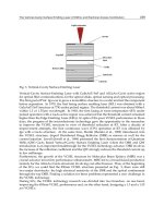
The force that can be generated by the thruster is characterized, as shown in Figure 8. The
significant linearity between the thruster force and the applied duty cycle will significantly
facilitate the design and implementation of any control scheme.


Fig. 8. Calibration of the motor: force with respect to duty cycle

A fluid drag force model is established to evaluate the speed that the AUV can achieve.
Figure 9. shows the relationship between the drag forces with respect to the relative velocity
of the vehicle. Under the full load of the two thrusters, the vehicle is able to achieve a
maximum forward or backward speed of 1.4m/s (~5km/hour).


Fig. 9. Drag force of the AUV with different velocities


Mobile Robots - State of the Art in Land, Sea, Air, and Collaborative Missions144
7.4 Ballast and depth control

Selection of a suitable ballast system is dependent on various factors, such as design
specifications, size and geometry of the AUV hull, depth required, and cost. In this design,
the hull is made of a PVC pipe with an outer diameter of 400mm and a length of 800mm.

The required working depth is 20m. Hence, the ballast system selected not only has to meet
the basic requirements enumerated above, but must also be able to fit in the hull. Preferably,
all are at a relatively low cost.
First, installing two (2) 160mm inner diameter ballast tanks of 250mm length provides a net
force of ±5kg. Additionally, the force required to actuate the piston head at 20m is calculated
to be approximately 6000N. To generate such force on the piston head, a powerful linear
actuator is needed. The specific linear actuator (LA36 24V DC input, 6800N max load,
250mm stoke length) can be sourced from Linak Ltd in New Zealand. However, the linear
actuator has a duty cycle of 20% at max, which means that for every 20s continuous work, it
must remain off for 80s before operating again, allowing the AUV to float uncontrolled. In
addition, the cost of one linear actuator is US$1036, which would imply that similar
actuators with longer duty cycles would cost a larger amount at this time.
Taking the second option, a hydraulic pumping system can be customized from Scarlett
Hydraulics Ltd, New Zealand. The overall system has dimensions of 500mm × 250mm ×
250mm. It consists of a 1.2KW DC motor, a pump, a 4L hydraulic fluid tank, two dual
solenoid valves and two cylindrical tanks. This system meets the required specifications, but
has some drawbacks. In particular, it occupies too internal space of the hull, and weighs
approximately 20kg (a significant addition of weight). In this case, the overall hydraulic
pumping system will cost up to approximately US$2264.
The third option air compressor system is cost effective and is easy to operate by controlling
the vent and blow valves. However, the lack of accuracy in controlling compressed gas is a
major disadvantage. In addition, performance and operating time are limited by the amount
of stored gas. In this design, a 10L tank would be needed to fulfil the changes in buoyancy.
In other words, a gas cylinder containing 10L of air compressed to at least 3bar is required
for a single diving and rising cycle. Hence, to refill the gas cylinder, the AUV must float to
the waters surface before all the air runs out or risk being lost. Regarding the on-site
requirement that the AUV should operate for hours, the air tank must either be much bigger
or far more highly pressurize, which leads to safety issues.
The fourth option thrusters are different from the previous three systems that all had to be
installed inside the AUV. In contrast, thrusters can be attached externally. Hence, sealing is

not as critical as it is for the other concepts. If the vehicle is trimmed positively buoyant, it is
also reasonably fail-safe, unlike the other three methods. Additionally, the thrusters can be
sourced from Pu Tuo Hai Qiang Ltd, Zhou Shan, China for US$55/unit, a reduction of 12-
20× in cost if two are used. Each thruster fits in a 215mm × 215mm × 80mm box, and is
driven by a 12V DC motor with a max thrust force of 5kg under water. By mounting the
desired number of thrusters, a wide range of motions can be controlled, such as pitch and
roll control.
Finally, each concept has its own advantages and disadvantages. Comparisons are
summarized in Table 3. In this design, the major driving factors for the selection of ballast
system are the cost and reliability. Piston ballast tank and thruster systems are reliable since
these two depth control methods have been widely employed in most autonomous
The State-of-Art of Underwater Vehicles – Theories and Applications 145

underwater vehicle development. Considering the cost, the thruster system is more effective.
Hence, the thruster system is chosen as the final design.


Diving
Tech
Installation Buoyancy Sealing Reliability
Overall
Cost *
Piston ballast
tanks
Static Internal
+ ve, - ve,
Neutral
Difficult
Used in most
remote submarines

$2500
Hydraulic
pumping
system
Static Internal
+ ve, - ve,
Neutral
Difficult Not reliable $2710
Air compressor Static Internal
+ ve, - ve,
Neutral
Difficult
Air on board is
limited,
compressed air
hard to handle
$420
Thrusters Dynamic External + ve None
Used in most
ROVs with big size

$500
Table 3. Ballast comparison. * The cost is estimated as an overall system

There are four thrusters vertically mounted around the AUV with one at each corner (See
Figure 7). Mounting four thrusters produces a total of 20kg thrust force at full load, and
allows a wide range of motion control. They enable the control of not only the vertical up
and down motion, but pitch and roll motions. To achieve this control, each thruster is
connected to a speed control module that can be controlled via a central microprocessor. By
inputting different digital signals, various forces thus speeds are generated. Therefore,

desired motion control can be obtained by different combinations.

7.5 Electronics and control

7.5.1. Power supply
For long term operation, this design must locate the power supply on-board, unlike many
current models that receive power over an umbilical link (Chardard & Copros, 2002). Since
all the systems onboard the AUV are electric, sealed lead acid batteries are chosen for the
power supply. These batteries have high capacity and can deliver higher currents, than
other types of rechargeable battery (Schubak & Scott, 1995; Bradley et al., 2001). They are
stable, inexpensive, mechanically robust and can work in any orientation, all of which are
important considerations in a vehicle of this type. To supply enough current for the entire
machine several batteries have to be joined together. Instead of adding dead weight to
achieve neutral buoyancy extra batteries can be added as needed so that the total operating
time of the AUV is higher than that required for a given application.
It is also highly desirable to locate the battery compartments separate from the main hull so
that they can be interchanged in the field without opening the sealed main hull. To
accommodate this requirement two tubes are fitted below the hull to house batteries. Within
these tubes the batteries are connected to two bus bars. Each battery is fused prior to
connecting to the bus bar, and the bars are isolated to the greatest extent possible to increase
safety. These bus bars are then wired into the main hull, where a waterproof socket enables
the quick interchange of battery compartments. A similar bus system exists inside the hull
Mobile Robots - State of the Art in Land, Sea, Air, and Collaborative Missions146
with connections to motors and electronic power supplies. Each of these internal
connections is similarly fused. Longer term, it would be desirable to intelligently monitor
the bus to track the state of each battery and overall power consumption.

7.5.2. Central processing unit
The central processing unit is responsible for accessing sensors, processing data and setting
control outputs such as motor speeds. Several systems are considered for this unit, an

embedded system using microprocessors, FPGAs or a small desktop PC. A microprocessor
system, most likely based on an ARM processor would have low cost, size and power
requirements and is easy to interface to both analogue and digital sensors, motors and other
actuators. The processing power and memory allocations of these microprocessors are all
more than sufficient for the simple control tasks likely to be required, but would struggle
with larger sensor or processing tasks, such as image processing. An FPGA system would
also be small and have low power requirements, but would be more expensive. While
FPGAs work very well for fast, complex processing tasks such as image processing, their
complexity in design and programming necessitates their use in parallel with other more
flexible CPU choices. The last system considered is a small desktop PC. Although a desktop
PC is bigger, more expensive and consumes more power than either of the prior two options,
it provides immense processing power, memory and a diverse range of peripherals. It is
therefore chosen in this initial design for the following primary reasons:
x Added power requirements were not an issue since we have a sizeable power
supplies.
x Processing power is more than adequate for this initial design and future
developments.
x Large volumes of memory are available, both volatile for program execution and
solid state for storage of gathered data.
x Despite not having direct access to sensors and control units, a diverse range of
peripherals available can be used, including USB, RS232 and Ethernet, enabling a
potentially greater range of sensors and sensor platforms for developing broad
ranges of specific applications.
x A USB module is already provided for a webcam for initial image sensing
applications and an Ethernet module is provided for remote connection.
An AMD Sempron 3000+ processor and ASUS M2N-PV motherboard are used for this
purpose. These models have lower power requirements and heat generation. Software
interfaces this unit with sensors and motor controllers, as well as to a remote control PC. An
automotive power supply (Exide, Auckland, NZ) is used to provide power for the computer.
It takes a 12V DC input and converts it to the ATX standard power supply required by the

PC. This module is also designed to be used in an electrically noisy and hostile environment
and is ideally suited the specific design situations considered.

7.5.3. Sensors
When the AUV is used autonomously, after development there will be a large and extensive
sensor suite onboard. Currently, the sensors onboard measure

x water pressure, from which depth can be determined
x water temperature, inner hull temperature and humidity
The State-of-Art of Underwater Vehicles – Theories and Applications 147

x the AUV position in the three principal axes: yaw, pitch and roll
x visual or digital image feedback via a webcam.
Submersible pressure sensors that are salt water tolerant and can measure up to the
pressures required are difficult to acquire at low cost. The sensor chosen was sourced from
Mandeno Electronics for US$121. This sensor measures up to twice the depth required, and
outputs an analogue output between 0 and 100mV. Thermocouples from Farnell Electronics
(Christchurch, New Zealand) are used to measure the water temperature, and provide an
analogue output relative to the temperature difference between the two ends of the
thermocouple. TMP100 sensors (Texas Instruments) are used to measure the base
temperature of the thermocouple, and the hulls interior temperature. These sensors give a
digital output using the I2C protocol. A HF3223 humidity sensor (Digi-Key) is used to
measure humidity inside the hull. A MMA7260QT accelerometer (Freescale Semiconductor)
is used to calculate orientation. The accelerometer has a 0-2.5V analogue output. The
connection of the sensors is shown in Figure 10.
To eliminate signal noise, An Atmel AT90USB82 microprocessor is connected to the USB
ports of the computer to move all noise sensitive data to the acquisition points. The
analogue sensors are amplified using an INA2322 instrumentation amplifier, if necessary,
and read by an ADS7828 analogue to digital converter. This converter is then connected to
the Atmel microprocessor using a common I2C bus with the TMP100. The humidity sensor

is attached to a clock input which converts the frequency based signal to a humidity based
reading. The microprocessor performs some basic processing on this data, temperature
compensating the pressure sensor and thermocouple, and calculating yaw, pitch and roll
from the accelerometer readings.


Fig. 10. The block diagram for electronic systems and control

Visual or digital image sensing is included via a Logitech webcam connected directly to the
on-board computers USB port. The video stream can be sent back over a wireless remote
control network connection to the remote PC. At this stage, no image processing is done on
this stream on-board, and it is included purely to assist in manual control of the AUV at this
time, and for use in later application development.
Mobile Robots - State of the Art in Land, Sea, Air, and Collaborative Missions148
7.5.4. Propulsion motor driver
For the six motors (two for horizontal propulsion, and four for vertical ballast control), three
(3) RoboteQ AX2500 motor controllers are used for control. Each controller is able to control
two motors up to 120 amps, much higher than the 25 amps needed by the motors selected.
The controllers are controlled via RS232 (serial port) interfaces, which are already available
on the computer motherboard. Computer control of the controllers is easily achieved
through a LabView or MATLAB interface, either manually or automatically, where both
interfaces have been implemented to allow greater user ease of use.

7.5.5. Control system and communications
During testing and development, remote control is required for the AUV. Sensors readings
need to be sent to a user, and control signals sent back to the AUV. Displaying the video
feed from the webcam is also desired to provide the operator with visual feedback. High
frequency radio transmissions are impossible underwater due to the high losses
encountered during the air/water boundary (Leonessa et al., 2003). Lower frequency
transmissions could have been used to communicate with the AUV, but they do not possess

enough bandwidth to send the required data. An umbilical Ethernet cable is being used for
this remote link between the AUV and an external control computer for this development
phase. Figure 6. shows the electronics and control structure. Note that in an actual,
developed application, or final development thereof, the robot will be acting autonomously
and this umbilical will not be required.

8. Conclusions and future work

AUVs have a lot of potential in the scientific and military use. With the development of
technologies, such as accurate sensors and high density batteries, the use of AUVs will be
more intensive in the future. In this book chapter, several subjects of an AUV have been
reported. For every subject some of the techniques used in the past and the techniques used
nowadays are described. For every aspect a suitable technique for an AUV is given. To show
how the state-of-the-art technologies could be used in AUVs, an AUV prototype developed
recently at the University of Canterbury has been detailed in design.
The AUV was specially designed and prototyped for shallow water tasks, such as inspecting
and cleaning sea chests of ships. It features low cost and wide potential use for normal
shallow water tasks with a working depth up to 20m, and a forward/backward speed up to
1.4m/s. Each part of the AUV is deliberately chosen based on a comparison of readily
available low cost options when possible. The prototype has a complete set of components
including vehicle hull, propulsion, depth control, sensors and electronics, batteries, and
communications. The total cost for a one-off prototype is less than US$10,000. With these
elements, a full range of horizontal, vertical and rotational control of the AUV is possible
including computer vision sensing. The overall underwater vehicle will be a good platform
for research, as well as for its specific applications, many of which are growing in
importance like the sea chest inspection case noted here.
The controls of the vehicle are under development. The vertical motion control uses the
feedback from the pressure sensor, while the horizontal motion control uses an inertial
measurement unit (Microstrain GX2 IMU, VT, USA) to get information about the vehicle
attitude and acceleration. The fluidic model (dynamic drag force) of the vehicle will be

The State-of-Art of Underwater Vehicles – Theories and Applications 149

established by simulation and verified by experimental measurement. This model would be
integrated in the control and navigation module of the vehicle.

9. References

Allmendinger, E. (1990). Submersible Vehicle Systems Design. Jersey City, NJ: Society of Naval
Architects and Maringe Engineers, 1990.
Ballard, R. (1987). The Discovery of the Titanic. New York, NY: Warner/Madison Press Books,
1987.
Blidberg, D. (2001). The development of autonomous underwater vehicles (AUV): a brief
summary, Proceedings of the IEEE International Conference on Robotics and Automation
(ICRA2001), Seoul, Korea, May 2001.
Bradley, A.; Feezor, M.; Singh, H. & Sorrell, F. (2001). Power systems for autonomous
underwater vehicles, IEEE Journal of Oceanic Engineering, Vol. 26, No. 4, 526–538.
Caccia, M. (2006). Autonomous surface craft: prototypes and basic research issues, 14th
Mediterranean Conference on Control and Automation, June 2006.
Cavallo, E. & Michelini, R. (2004). A robotic equipment for the guidance of a vectored
thrustor AUV, 35th International Symposium on Robotics ISR 2004, 2004.
Chardard, Y. & Copros, T. (2002). Swimmer: final sea demonstration of this innovative
hybrid AUV/ROV system, Proceedings 2002 International Symposium on Underwater
Technology, Tokyo, Japan, Apr. 2002, 17-23.
Curtin, T. & Bellingham, J. (2001). Autonomous ocean-sampling networks, IEEE Journal of
Oceanic Engineering, Vol. 26, 421-423.
Evans, J. & Meyer, N. (2004). Dynamics modeling and performance evaluation of an
autonomous underwater vehicle, Ocean Engineering, Vol. 31, 1835-1858.
Fauske, K.; Gustafsson, F. & Hegrenaes, O. (2007). Estimation of AUV dynamics for sensor
fusion, 10th International Conference on Information Fusion 2007, 1-7, July 2007.
Feng, Z. & Allen, R. (2004). Reduced order H1 control of an autonomous underwater

vehicle, Control Engineering Practice, Vol. 12, 1511-1520.
Fossen, T. (1994). Guidance and control of ocean vehicles. New York: John Wiley and Sons Ltd.,
2-nd ed., 1994.
Fryxell, D.; Oliveira, P.; Pascoal, A.; Silvestre, C. & Kaminer, I. (1996). Navigation, guidance
and control of AUVs: an application to the MARIUS vehicle, Control Engineering
Practice, Vol. 4, No. 3, 401-409.
Gaccia, M. & Veruggio, G. (2000). Guidance and control of a reconfigurable unmanned
underwater vehicle, Control Engineering Practice, Vol. 8, 21-37.
Griffiths, G. & Edwards, I. (2003). AUVs: designing and operating next generation vehicles,
Elsevier Oceanography Series, Vol. 69, 229-236.
Haberbusch, M.; Stochl, R.; Nguyen, C.; Culler, A.; Wainright, J. & Moran, M. (2002).
Rechargeable cryogenic reactant storage and delivery system for fuel cell powered
underwater vehicles, Proceedings Workshop on Autonomous Underwater Vehicles, 103-
109, June 2002.
Horgan, J. & Toal, D. (2006). Review of machine vision applications in unmanned
underwater vehicles, 9th International Conference on Control, Automation, Robotics and
Vision, Dec. 2006.
Mobile Robots - State of the Art in Land, Sea, Air, and Collaborative Missions150
Hsu, C.; Liang, C.; Shiah, S. & Jen, C. (2005). A study of stress concentration effect around
penetrations on curved shell and failure modes for deep-diving submersible
vehicle, Ocean Engineering, Vol. 32. No. 8-9, 1098-1121.
Jalbert, J.; Baker, J.; Duchesney, J.; Pietryka, P.; Dalton, W.; Blidberg, D.; Chappell, S.; Nitzel,
R. & Holappa, K. (2003). A solar-powered autonomous underwater vehicle,
OCEANS 2003.
Jalving, B. (1994). The NDRE-AUV flight control system, IEEE Journal of Oceanic Engineering,
Vol. 19, 497-501.
Kaminer, I.; Pascoal, A.; Khargonekar, P. & Coleman, E. (1995). A velocity algorithm for the
implementation of gain-scheduled controllers, Automatica, Vol. 31, No. 8, 1185-1191.
Keary, A.; Hill, M.; White, P. & Robinson, H. (1999). Simulation of the correlation velocity
log using a computer based acoustic model, 11th International Symposium Unmanned

Untethered Submersible Technology, 446-454, August 1999.
Kondoa, H. & Ura, T. (2004). Navigation of an AUV for investigation of underwater
structures, Control Engineering Practice, Vol. 12, 1551-1559.
Lee, P.; Jun, B.; Kim, K.; Lee, J.; Aoki, T. & Hyakudome, T. (2007). Simulation of an inertial
acoustic navigation system with range aiding for an autonomous underwater
vehicle, IEEE Journal of Oceanic Engineering, Vol. 32, 327-345.
Leonard, J.; Bennett, A.; Smith, C. & Feder, H. (1998). Autonomous underwater vehicle
navigation, Proceedings IEEE ICRA Workshop Navigation Outdoor Autonomous Vehicle,
May 1998.
Leonessa, A.; Mandello, J.; Morel, Y. & Vidal, M. (2003). Design of a small, multi-purpose,
autonomous surface vessel, Proceedings OCEANS 2003, Vol. 1, San Diego, CA, USA,
2003, 544–550.
Lygouras, J.; Lalakos, K. & Tsalides, P. (1998). THETIS: an underwater remotely operated
vehicle for water pollution measurements, Microprocessors and Microsystems, Vol. 22,
No. 5, 227–237.
Majumder, S.; Scheding, S. & Durrant-Whyte, H. (2001). Multisensor data fusion for
underwater navigation, Robotics and Autonomous Systems, Vol. 35, 97-108.
Maurya, P.; Desa, E.; Pascoal, A.; Barros, E.; Navelkar, G.; Madhan, R.; Mascarenhas, A.;
Prabhudesai, S.; Afzulpurkar, S.; Gouveia, A.; Naroji, S. & Sebastiao, L. (2007).
Control of the Maya AUV in the vertical and horizontal planes: theory and practical
results, Proceedings MCMC2006 - 7th IFAC Conference on Manoeuvring and Control of
Marine Craft, 2007.
Modarress, D.; Svitek, P.; Modarress, K. & Wilson, D. (2007). Micro-optical sensors for
underwater velocity measurement, Symposium on Underwater Technology and
Workshop on Scientific Use of Submarine Cables and Related Technologies, 235-239, April
2007.
Monteen, B.; Warner, P. & Ryle, J. (2000). Cal poly autonomous underwater vehicle,
California Polytechnic State University, 2000.
Paster, D. (1986). Importance of hydrodynamic considerations for underwater vehicle
design, OCEANS, Vol. 18, 1413-1422, September 1986.

Ridao, P.; Batlle, J. & Carreras, M. (2001). Model identification of a low-speed AUV, In
Control Applications in Marine Systems. International Federation on Automatic
Control, 2001.
The State-of-Art of Underwater Vehicles – Theories and Applications 151

Rife, J. & Rock, S.M. (2002). Field experiments in the control of a jellyfish tracking ROV, in
MTS/IEEE Oceans ’02, Vol. 4, 2002, 2031-2038.
Ross, C. (2006). A conceptual design of an underwater vehicle, Ocean Engineering, Vol. 33,
No. 16, 2087-2104.
Schubak, G. & Scott, D. (1995). A techno-economic comparison of power systems for
autonomous underwater vehicles, IEEE Journal of Oceanic Engineering, Vol. 20, No. 1,
94-100.
Serrani, A. & Conte, G. (1999). Robust nonlinear motion control for AUVs, IEEE Robotics &
Autonomation Magazine, Vol. 6, 33-38.
Smallwood, D. & Whitcomb, L. (2004). Model-based dynamic positioning of underwater
robotic vehicles: theory and experiment, IEEE Journal of Oceanic Engineering, Vol. 29,
No. 1, 169-186.
Smallwood, D.; Bachmayer, R. & Whitecomd, L. (1999). A new remotely operated
underwater vehicle for dynamics and control research, Proceedings UUST ’99, 1999.
Smith, P.; James, S. & Keller, P. (1996). Development efforts in rechargeable batteries for
underwater vehicles, Proceedings Autonomous Underwater Vehicle Technology
Symposium, AUV'96, 441-447, June 1996.
Stachiw, J. (2004). Acrylic plastic as structural material for underwater vehicles, International
Symposium on Underwater Technology, 289-296, April 2004.
Stutters, L.; Liu, H.; Tiltman, C. & Brown, D. (2008). Navigation technologies for
autonomous underwater vehicles, IEEE Transactions on Systems, Man and
Cybernetics, Part C: Applications and Reviews, Vol. 38, 581-589.
Takagawa, S. (2007). Feasibility study on DMFC power source for underwater vehicles,
Symposium on Underwater Technology and Workshop on Scientific Use of Submarine
Cables and Related Technologies, 326-330, April 2007.

Tangirala, S. & Dzielski, J. (2007). A variable buoyancy control system for a large AUV, IEEE
Journal of Oceanic Engineering, Vol. 32, 762-771.
Tivey, M.; Johnson, H.; Bradley, A. & Yoerger, D. (1998). Thickness of a submarine lava flow
determined from near-bottom magnetic field mapping by autonomous underwater
vehicle, Geophysical Research Letters, Vol. 25, 805-808.
Toal, D.; Flanagan, C.; Lyons, W.; Nolan, S. & Lewis, E. (2005). Proximal object and hazard
detection for autonomous underwater vehicle with optical fibre sensors, Robotics
and Autonomous Systems, Vol. 53, 214-229.
Uhrich, R. & Watson, S. (1992). Deep-ocean search and inspection: Advanced unmanned
search system (AUSS) concept of operation, Naval Command, Control and Ocean
Surveillance Center, RDT&E Division, San Diego, CA, Tech. Rep. NRaD TR 1530,
Nov. 1992.
Valavanis, K.; Gracanin, D.; Matijasevic, M.; Kolluru, R. & Demetriou, G. (1997). Control
architectures for autonomous underwater vehicles, Control Systems Magazine, Vol.
17, 48-64.
von Alt, C. (2003). Autonomous underwater vehicles, Autonomous underwater Langrangian
platforms and sensors workshop, LaJolla, CA, March-April 2003.
Wasserman, K.; Mathieu, J.; Wolf, M.; Hathi, A.; Fried, S. & Baker, A. (2003). Dynamic
buoyancy control of an ROV using a variable ballast tank, OCEANS 2003, Vol. 5,
SP2888-SP2893, September 2003.
Mobile Robots - State of the Art in Land, Sea, Air, and Collaborative Missions152
Wernli, R. (2001). Low cost AUV’s for military applications: Is the technology ready? in
Pacific Congress on Marine Science and Technology 2001, San Francisco, CA, July 2001.
Willcox, S.; Vaganay, J.; Grieve, R. & Rish, J. (2001). The bluefin BPAUV: An organic wide-
area bottom mapping and mine-hunting vehicle, in Proceedings UUST ’01, 2001.
Williams, C. (2004). AUV systems research at the NRC-IOT: an update, in 2004 International
Symposium on Underwater Technology, 2004, 59-73.
Williams, S.; Newman, P.; Dissanayake, G.; Roseblatt, J. & Durrant-Whyte, H. (2006). A
decoupled, distributed AUV control architecture, University of Sydney NSW, 2006.
Wilson. R. & Bales, J. (2006). Development and experience of a practical pressure-tolerant,

lithium battery for underwater use, OCEANS 2006, 1-5, September 2006.
Winchester, C.; Govar, J.; Banner, J.; Squires, T. & Smith, P. (2002). A survey of available
underwater electric propulsion technologies and implications for platform system
safety, Proceedings Workshop on Autonomous Underwater Vehicles, 129-135, June 2002.
Wolf, M. (2003). The design of a pneumatic system for a small scale remotely operated vehicle,
Bachalor’s Thesis, MIT, May 2003.
8

General Concept of 3D SLAM

Peter Zhang, Evangelous Millos & Jason Gu
Dalhousie University
Canada


Simultaneous localization and mapping (SLAM) is a process that fuses sensor observations
of features or landmarks with dead-reckoning information over time to estimate the location
of the robot in an unknown area and to build a map that includes feature locations. In this
chapter, a general model and its related solving algorithm for 3D SLAM are established. The
method can be used for all of the situations in the mobile robot community. An underwater
mobile robot is used as an example.
This chapter is organized as follows: Section 1 is the problem definition; Section 2 establishes
all the models for 3D SLAM, including the robot process model, the landmark model, and
the measurement model; Section 3 is the method for data association; Section 4 presents the
algorithms to solve the SLAM; section 5 describes the multi-sensor related issues based on
the underwater mobile robot cases; and Section 6 is the globally-consistent 3D SLAM for
mobile robot in real environment.

1. Problem Definition


Assuming a 3D environment with randomly distributed landmarks and an autonomous
mobile robot equipped with sensors (stereo camera, laser range finder, or sonar) which will
move in this environment, by providing some proper input (robot speed and orientation),
we need to determine the robot pose (position and orientation) and the position of detected
landmarks during the robot navigation. Because of measurement noise and robot input
noise, it is very difficult to compute a deterministic value for the robot pose and landmark
position. We can only estimate their approximate value by using algorithms such as the
Kalman filter, the Particle filter, and the Unscented Kalman filter. By using these algorithms,
it is also possible to calculate the confidence of the estimation. In some areas of the robot’s
working environment, significant landmarks are sparse, especially in the underwater
environment. A robot equipped with only one type of sensor may not obtain sufficient
effective measurements, which would greatly affect the accuracy of the robot pose; therefore,
more than one sensor will be used for the robot navigation in a real application. In this
thesis, the SLAM problem in the 3D environment will be solved with multiple
heterogeneous sensors. A general strategy will be proposed and related algorithms will be
developed.


Mobile Robots - State of the Art in Land, Sea, Air, and Collaborative Missions154
2. Models for 3D SLAM

2.1. Robot Process Model
Robot process model is a dynamic differential equation to describe the movement of a robot
in a given environment and system input. It is related to the robot pose. The robot pose can
be determined by its position and orientation. In a global coordinate system OXYZ, a robot
position (p
v
) is expressed by (x, y, z)
T
, , and its orientation can be expressed by Euler angles,

rotation matrix, axis and angle, or quaternion. From any one of the orientation
representations, it is possible to compute the other representations. For simplicity, Euler
angles are selected as a robot orientation state vector. Therefore, the state vector of the robot
X
v
can be expressed as


»
»
»
»
»
»
»
¼
º
«
«
«
«
«
«
«
¬
ª

»
¼
º

«
¬
ª

z
y
x
T
v
T
v
v
z
y
x
p
X
T
T
T
T
(1)

where T is the transpose of a matrix and assuming that the robot moves relative to its
current pose with speed v and changes direction with Euler angles (
zyx
G
T
G
T

G
T
,,
), the
input to the robot can be expressed by

»
»
»
»
¼
º
«
«
«
«
¬
ª

z
y
x
v
U
GT
GT
GT
(2)

where v is the robot speed in scalar, and the direction of the speed is always in the robot's

forward pointing axis of its body. In order to simplify its implementation, the Euler angles
need to be expressed in the form of a rotation matrix M
v

)()()(
zzyyzzv
RRRM
T
T
T

(3)

where Rz, Ry, and Rx are the rotation matrices which are the rotation around the z, y, x-axis,
respectively, in right hand coordinate system with positive angle
zyz
T
T
T
,,
, the positive
angle is at counter-clockwise direction. Then, the robot process model can be expressed as

»
»
»
¼
º
«
«

«
¬
ª

»
»
»
¼
º
«
«
«
¬
ª




),,),((
),,),((
),,),((
)1(
)1(
)1(
)1(
3
2
1
zyxz
zyxy

zyxx
z
y
x
u
kf
kf
kf
k
k
k
k
GTGTGTT
GTGTGTT
GTGTGTT
T
T
T
T
(4)
and

General Concept of 3D SLAM 155
tvkM
kz
ky
kx
kz
ky
kx

kP
uu
G
J
E
D
»
»
»
¼
º
«
«
«
¬
ª

»
»
»
¼
º
«
«
«
¬
ª

»
»

»
¼
º
«
«
«
¬
ª




)cos(
)cos(
)cos(
)(
)(
)(
)(
)1(
)1(
)1(
)1(
(5)

where
t
G
is the sampling time, M
v

(k) is the rotation matrix, which corresponds to the Euler
angles
)(),(),( kkk
zyx
T
T
T
at time k. In Equation(4), the angle
)1( k
v
T
corresponds to
the matrix Mv(k + 1), which has following equation

)()()1( kMMkM
vvv
 
G
T
(6)
where
)(
G
T
v
M
is a matrix which corresponds to the Euler angle
G
T
and in Equation.(5),

And the
J
E
D
,,
are direction angles corresponding to the Euler angles,
)(),(),( kkk
zyx
T
T
T
.

By combining the Equation(4) and (5), the process model can be written as a non-linear
equation

)()()(),(()1( kkkUkXFkX
uu
Z
P
 
(7)

where
)(k
P
the input is noise, and
)(k
Z
is the process noise, at the sample time k. The

noise is assumed to be independent for different k, white, and with zero mean and
covariance Q
v
(k).


Fig. 1. Coordinate systems of an autonomous mobile robot.





Mobile Robots - State of the Art in Land, Sea, Air, and Collaborative Missions156
2.2. Landmark Models
Landmarks can be classified into two types, artificial and natural. In a newly-visited natural
environment, there is no artificial landmark for mobile robot navigation; therefore the
natural landmarks are the only choice.


Fig. 2. General landmark expression.

A robot map consists of a set of landmarks. In order to provide enough information for
robot navigation, every landmark should include position information and attribute
information (Figure. 2). If the landmark position is known, a sensor’s measurement of it can
be used in the robot pose estimation with algorithms such as the extended Kalman filter or
the particle filter. If the landmark position is unknown, an algorithm for SLAM will be
applied to estimate the robot pose and landmark position by the aid of measurements. The
attribute information will provide knowledge about the landmark which distinguishes it
from other features, which is very useful for data association; therefore, landmark Li can be
expressed as


>
@
attributeipositionii
LLL
,,

(8)
where

»
»
»
¼
º
«
«
«
¬
ª

i
i
i
ipositioni
z
y
x
LL
,

. (9)

During robot navigation, even though its environment is unknown, the landmarks for a
map establishment are always assumed to have a static position. It is also assumed that
attributes (or features) of a landmark will not change. In reality, features of a landmark may
change with lighting conditions and sensor view point, therefore, the landmark i has the
following evolution equation
General Concept of 3D SLAM 157
)()1( kLkL
ii

(10)

where
mi ,,1 !
, which means there are m landmarks which will be used; k is the time
which is used during the robot navigation.

2.3. Measurement Model
A mobile robot is always equipped with some type of sensors for its navigation. The sensors
can obtain measurements of the relative location of the observed landmarks with respect to
the robot. This observation can be expressed by a set of non-linear functions of the
landmark’s position relative to the robot position, which is called measurement model.
Assuming the position of landmark i in the global coordinate system OXYZ is (
iii
zyx
,
,
).
At time k, the robot has the pose

)(kX
u
. The measurement of the landmark i at this time
can be computed by

»
»
»
¼
º
«
«
«
¬
ª




»
»
»
¼
º
«
«
«
¬
ª


)(
)(
)(
)(
)(
)(
)(
kzz
kyy
kxx
kM
kZ
kZ
kZ
Z
i
i
i
v
z
y
x
i
i
i
i
. (11)
The observation model in the non-linear equation is

)())(),(()(),,),(( kkLkXhkzyxkXhZ

iviiivi
K
K
 
(12)

where
)(k
K
is the observation noise, which is assumed with zero mean and covariance R
i

and h(·) is the non-linear measurement function.
Without loss of generality, it is assumed that the measurement from every sensor is
independent. If there are m features observed at time k, the measurement model is obtained
by simply stacking Equation. (12) as

)())(),((
)(
)(
)(
)(
2
1
kkLkXH
kZ
kZ
kZ
kZ
v

m
K

»
»
»
»
¼
º
«
«
«
«
¬
ª

"
. (13)

An instance of a robot and five landmarks in 3D space is shown in Figure 3. When the robot
moves in space, its sensor detects landmarks which are located in the view field of the
sensor, then the robot pose and landmark position estimation can be performed. The
estimated landmark position will be used to build a map which can be used by the robot for
future navigation.

Mobile Robots - State of the Art in Land, Sea, Air, and Collaborative Missions158

Fig. 3. An instance of a robot and features in 3D experiment case.

3. Data Association


There are two types of data associations - measurement between sensors received from
multi-sensors, and measurement between adjacent times from a single sensor. In this thesis,
only the data association between adjacent times from a single sensor will be addressed.
During robot navigation, if the sensor on the robot only observed one landmark, there
would be no need for data association. Most sensors, such as camera, radar, laser, and sonar,
will detect not only many real landmarks, but also many spurious landmarks; therefore,
data association is a necessary step for landmark-based robot localization and object
tracking.
A landmark defined in the previous Section 2.2. includes position and attributes (feature)
components. If the attribute tuple is available, then data association can be implemented
with this information; otherwise, maximum likelihood of measurement will be used.

3.1. Data Association by Feature Attribute
Data association by using the landmark’s attribute is simple. A very good example is the
image feature registration with SIFT (Scale Invariant Feature Transforms) features (Se et al.,
2003). SIFT features in an associated image are among the best representations for the
natural unstructured environment. The SIFT features are invariant to image scaling,
translation, and rotation, and partially invariant to illumination changes and affine or 3D
projection. The structure of the SIFT feature is as follows:

[u, v, gradient, orientation, descriptor1, · · · , descriptorM]


where M is the number of the descriptor in SIFT feature. The position of landmark and the
position of its related SIFT features (in an image) of a landmark have a non-linear relation. If
a camera’s physical position and orientation are given, the position of the landmark
associated with the SIFT feature can be calculated by using its associated camera model
(Sonka et al., 1999).
General Concept of 3D SLAM 159


Fig. 4. SIFT features in an image.

An example of SIFT features in an image is shown in Figure 4. The data association for SIFT
features can be carried out by using their feature descriptor directly. SIFT features
correspondence between two adjacent images obtained from a moving camera at different
view points after the implementation of data association is displayed in Figure 5.
Mobile Robots - State of the Art in Land, Sea, Air, and Collaborative Missions160

Fig. 5. Result of SIFT feature correspondence between two adjacent images obtained from a
moving camera at different view points after data association.

3.2. Data Association by Maximum Likelihood of Measurement
If the measurements only provide a landmark’s position information, but the landmark’s
attribute information is empty, the method presented by Bar-Shalom et al. (Bar-Shalom &
Fortmann, 1998) for the data association with innovation will be used here. Their method
can be briefly described as follows:

Innovation is the value of difference between measurement Z(k) and predicted
measurement
)(kZ

, and expressed by
)(k
Q


)()()( kZkZk



Q
. (14)

In order to define a measurement validation region, the innovation needs to be normalized
as follows:

General Concept of 3D SLAM 161
)()()()(
1
kkSkk
v
T
v
QQH


(15)

where
)(kS
v
is the innovation covariance matrix, and it is defined as

)()()()()( kRkHkPkHkS
v
T
vv

(16)


where
)(kP
v
is the state vector’s estimated covariance matrix at step k, and
)(k
v
H
has a
2
F
distribution with
z
n
degrees of freedom (
z
n
is the dimension of the measurement Z).
The validation technique is based on this innovation. If a measurement is inside a fixed
region of a
2
F
distribution, then this observation is accepted; otherwise the observation is
rejected.

4. Estimation of Robot Pose and Landmark Positions

In the SLAM problem, a robot pose and landmark positions at time k+1 are unknown. They
need to be estimated by using input information U, measurement information Z, and robot
pose and feature position information, at time k. Stacking Equation (4) and Equation (5), the
system process model can be expressed as


»
¼
º
«
¬
ª


»
¼
º
«
¬
ª



»
»
»
»
»
»
¼
º
«
«
«
«

«
«
¬
ª





)(
)())(),(),((
)1(
)1(
)1(
)1(
)1(
)1(
)1(
2
1
kL
kkkUkXF
kL
kX
kL
kL
kL
kX
kX
vv

m
v
s
ZP
#
(17)
and the measurement model is

)())(),(()( kkLkXHkZ
v
K

. (18)

Both process model (Equation(17)) and measurement model (Equation(18)) are nonlinear
equations. A straightforward method to solve this problem is the Extended Kalman Filter
(EKF). Due to the high dimensions of the state vector and the need for linearization of the
non-linear models, the EKF is not computationally attractive. The particle filter-based fast
SLAM approach will be applied to solve this problem.

4.1. Particle Filter
From the view point of probability, the estimation of a robot pose and landmark positions
involves computing their posterior probability density function (PDF),
))1(),1(),(|)(),((  kUkXkZkLkXp
vv
, based on the prior probability density
function
))(|)(( kXkZp
v
and

))2(),2(),1(|)1((  kUkXkZkXp
vv
,
Mobile Robots - State of the Art in Land, Sea, Air, and Collaborative Missions162
where
)(kX
v
is the robot state, L(k) is the landmark state, Z(k) is the measurement, U(k) is
the input to the system, at time k. This is the well-known Bayesian approach. According to
the definition of a robot model and landmark model in the previous section 3.2, the PDF for
a SLAM problem
))1(( kXBel
v
at time k+1 can be defined as (Thrun & Burgard, 1998)

))()),(),1(|)1(())1(( kUkXkZkXpkXBel
vvv
 
. (19)

The solution for the SLAM problem is to estimate the maximum of the
))1(( kXBel
v

Bayes’ formula can be used on Equation (19) to simplify its implementation.

))(),(|)1((
))(),(|)1(())(),(),1(|)1((
))1((
kUkXkZp

kUkXkXpkUkXkXkZp
kXBel
v
vvvv
v



))(),(|)1(())(),(),1(|)1(( kUkXkXpkUkXkXkZp
vvvv

[
(20)

where
[
is the value of the inverse denominator and is assumed to be a constant. It is
known that the measurement Z(k + 1) is only dependent on the current pose
)1( kX
v
and is not influenced by previous pose
)(kX
v
and robot movement U(k).
Therefore, Equation. (20) can be simplified into

))(),(|)1(())(),(),1(|)1(())1(( kUkXkXpkUkXkXkZpkXBel
vvvvv
 
[


(21)

By applying the total probability theorem to the second item of the right hand side of
Equation (21), then

)1(|)1(())1((   kXkZpkXBel
vv
[

)())1(),1(),(|)(())(),(|)1(( kdXkUkXkZkXpkUkXkXp
vvvvv

³
(22)

³
  )())(())(),(|)1(()1(|)1(())1(( kdXkXBelkUkXkXpkXkZpkXBel
vvvvvv
[

(23)
where
))1(|)1((  kXkZp
v
is the sensor observation model, which can be calculated
from Equation (18);
))(),(|)1(( kUkXkXp
vv


is the system evolution model, which
can be calculated from Equation (17). The integration in the Equation (23) is a difficult
challenge to solve the SLAM problem efficiently; therefore, a new algorithm must be
designed.
The Monte Carlo based particle filter can be used to overcome the implementation challenge
in Equation (23). In the particle filter,
))(( kXBel
v
is expressed as a set of particles and
every particle is propagated in time according to the state process model such as Equation
General Concept of 3D SLAM 163
(17). The weight of every particle is calculated based on the observation model from the
Equation (18). The robot pose and landmark position can be computed from the sum of the
weighted samples. The particles should be re-sampled for the next step’s estimation.
Implementation of a particle filter is summarized in Algorithm.1.

Input: Robot movement U(k), sensor measurement Z(k+1) and sample number
N
Output: Robot pose and features position


1: initialize state with p(X
v
(0))
2: repeat
3: for every particle i do
4: assign distribution using p(X
v
(k+1)|Xv(k),U(k)
5: end for

6: for every particle i do
7: compute weight w, using p(Z(k+1)|X
v
(k+1)
8: end for
9: calculate robot pose & landmark position from particles & associated weight
10: re-sample the particles
11: until robot stop navigation
Alg. 1. Particle filter implementation for robot pose and feature position

Particle filtering can be used for any process and observation models. In the Kalman filter
and the extended Kalman filter, the basic requirement is that the error of process model and
observation model should be Gaussian distribution. In most cases, this requirement is too
restrictive. The particle filter has been called bootstrap filter (Gordon, 1997), condensation
(Isard & Blake, 1998), or Monte Carlo filter (Dellaert et al., 1999). In recent years, this method
has been successfully used in problems of object tracking (Hue et al., 2002) and mobile robot
localization (Dellaert et al., 1999) (Thrun et al., 2001).

4.2. Fast SLAM
Fast SLAM is an approach to separate the SLAM problem into a robot pose and landmark
position estimation that is conditioned on the robot pose. The term was first introduced in
(Montemerlo et al., 2002). The implementation of FastSLAM is an example of the Rao-
Blackwellised particle filter (Doucet et al., 2000) (Murphy, 1999).
Mobile Robots - State of the Art in Land, Sea, Air, and Collaborative Missions164
Input: Robot movement U{k), sensor measurement Z(k + 1). and sample number
N

Output: Robot pose and detected features position

1: initialize state with p(X

v
(0))
2: repeat
3: for every particle i do
4: proposal distribution using p(X
v
(k+1)|X
v
(k),U(k)
5: end for
6: obtain observations Z(k + 1)
7: data association for the observation data
8: for every particle i do
9: compute weight using p(Z(k+1)|X
v
(k+1))
10: end for
11: re-sample the particles
12: if current observed feature exists in the map then
13: for every particle i do
14: for every observed feature do
15: update the state of the robot
16: end for
17: end for
18: end if
19: if current observed feature is not in the map (new detected features) then
20: for every particle i do
21: add the new detected features to the map based on the robot pose and observation
to the features
22: end for

23: end if
24: until robot stop navigation
Alg. 2. FastSLAM implementation

From the previous definition of a SLAM problem, the system state estimation could be
written as

))()),(),1(|)1(),1(())1(( kUkXkZkLkXpkXBel
vvv
 
(24)

This expression can be factored into two parts according to [8].



 
m
i
vivvv
kUKZkXkLpkUkXkZkXpkXBel
0
))(),1(),1(|)1(())()),(),1(|)1(())1((

(25)
The estimate expression is decomposed into m+1 estimations. One of them is for the robot
pose estimation, and m of them are for landmark estimation based on the estimated robot
pose. The implementation of FastSLAM is summarized in Algorithm 2. In this thesis, this
General Concept of 3D SLAM 165
algorithm is applied for the SLAM problem. The particle filter is implemented to calculate

its related conditional densities for robot and landmarks.


Fig. 6. SLAM implementation with features observed by a sensor.

The idea for FastSLAM can be obtained from Figure 6. We assume that all the observed
landmarks by a sensor at robot position
)1( kX
v
exist in a map. Then, the observed
landmarks at robot position
)(kX
v
can be divided into two groups. Some of them are
already in the map and are labeled as small yellow squares in Figure 6, which are called old
landmarks; some of them are new landmarks and do not yet exist in the map and are
expressed with small black dots in Figure 6. The measurements from the old landmarks are
applied for the robot pose estimation at time k. The measurements from the new landmarks
are used to estimate the new landmark positions in the global coordinate system based on
the robot position. Then, all the new landmarks are added into the map.
In the fast SLAM approach, the factorizing assumption step turned the high dimension 6 +
3 · m of the SLAM problem into the low dimension (6 and 3) problem’s combination, which
greatly improves the computation efficiency, but it is assumed that the estimated robot pose
has an accurate value. This assumption is not true and will cause errors in the step for the
landmark position estimation in a global frame. This is the trade-off between efficiency and
accuracy.
Another assumption in the fast SLAM is that the measurement of every detected landmark
is independent of the other landmarks in the working area of the robot; therefore, the
covariance between two landmarks will be zero. In other methods, such as the EKF or
Particle filter, robot pose and all the detected features position are estimated in one state

vector, and this may cause the covariance between two landmarks to be other than zero. In
most of the cases, these values came from the algorithm design.