Computer graphics
systems
5/31
are defined, either textual entry or schematic capture methods
can be used. Experienced users will often prefer textual entry,
being a faster method (especially for repetitive features) and
in which error checking
is
simplified. This method only
requires the use of a keyboard for data entry. Inexperienced
users tend to prefer
a
direct representation where they can see
what they are drawing.
If
a hard-copy output is required, this
is often the only suitable technique. For schematic entry
systems
a
pointer device is required to enter coordinates
to
the
system and such devices are described below. Pointer devices
are often used in conjunction with a keyboard in order to enter
data by the most efficient means for greater productivity.
However, they may sometimes be used alone.
Mouse, tracker ball, cursor key and joystick
These are
devices capable of passing orthogonally related coordinates to
the application. All except the cursor keys are able to enter

two coordinates simultaneously. Cursor keys are usually part
of the keyboard assembly and are the slowest of the above
devices to use. The amount that the coordinate is incremented
for each depression
of
the key is usually variab!e
to
give coarse
and fine positioning of the desired point.
A
mouse device contains a small ball which is moved across
the surface of a desk. The movement of the ball is detected
optically or mechanically and is converted to digital pulses, the
number and rate
of
which determine the distance
to
move and
the rate
of
movement. The mouse often contains switches
so
that the terminal position can be marked.
In
this way, the
mouse can be driven ‘single-handed’. Using a mouse requires
a free area of around 300
x
300 mm.
To overcome this restriction, the tracker ball inverts the

mouse
so
that the ball is moved directly by hand. The body
of
the tracker ball does not move but the ball may be freely
moved in any direction without limit. Again, switches may be
fitted to make a self-contained input device.
A
joystick operates in a similar way to the tracker ball
except that movement of the joystick arm
is
limited to a few
centimetres either side of
a
central position. The joystick may
be biased
to
return to the central position when pressure is
removed. Because of the limitation
of
movement
of
the
joystick, it is more useful where absolute positioning
is
re-
quired, whereas the mouse or tracker ball indicate
a
relative
position. However, using velocity sensing for the joystick, this

limitation may be overcome.
Graphics tablet
The graphics tablet represents a drawing
area where information
is
transferred to the application. The
tablet has sensors embedded in its surface which detect the
position of
a
stylus. These sensors are often arranged in a
matrix. When used with a stylus, data are entered free-hand in
much the same way
as
a user would sketch
a
design using
pencil and paper. The stylus may have
a
switch in the tip
so
that pressing the stylus indicates
a
selection. When existing
drawings are to be digitized, these are attached to the tablet
and reference points on the drawing are converted to coor-
dinates using a cross-hair device and switch. The application
can then use the reference points to recreate the drawing.
When used in this way, the graphics tablet
is
more commonly

known as
a
digitizer. The graphics tablet area may also have a
reserved space around its perimeter which is not used for
drawing, but which is divided into small areas used for the
selection
of
parameters.
Light-pen and touch screen
These operate in a similar
way
to
the graphics tablet, except that the monitor screen is used. The
light-pen detects the light generated when the
CRT
electron
beam strikes the phosphor coating and the position of the pen
is determined from the timing of the electricai pulse gener-
processing.
A
digitizing tablet is used to extract information
from existing documents rather than merely to scan the whole
image and
so
this requires a human operator. The pointer
(usually
a
cross-hair device) selects the major features of the
document and the coordinates of these points are transferred
to the processing system where the image feature may be

reconstructed.
Drawing
The drawing operation takes the image parameters
and converts them into a set of pixels in the frame buffer which
define the dispiay. The frame buffer contents are then a map
of what
is
seen on the output device and this is therefore a
bit-map
or
pixel-map
of
the image.
Converting the image parameters into pixels is not always
simple. The change from
a
continuous function such
as
a
straight line
to
a discretized version (pixels
on
a
screen) can
create unusual effects which are discussed in Section 5.3.4.2.
Graphics processors
Processing graphical data requires con-
siderable processing power.
If

this processing is performed in
software then the range of processing operations is large,
limited only by the ability of the programmer. The more
computing-intensive the operation, the more the throughput
suffers, in terms of frames processed per second. One way of
alleviating the problem is to perform some processing opera-
tions using dedicated hardware. Such devices include con-
volvers for filtering and masking images and SIMD or MIMD
devices for post-processing images. Parallel-processing tech-
niques are used to increase the speed of these computing-
intensive operations.
In
addition to the architectures men-
tioned above, the transputer is often used for graphics applica-
tions.
Colour look-up tables (palettes)
If
a
display were
to
offer
a
realistic range of colours then the information that would need
to
be stored would require a very large frame buffer. Fortu-
nately, not
all
colours need
to
be available at once in a given

image. ]For example, a programmer may select 64 out
of
4096
possible colours. This implies that while the system is capable
of representing 4096
physical
colours, only
64
logical
colours
are used.
A
means of mapping the logical colours to the
physical colours is provided by the Colour Look-up Table
(CLUT)
or
Palette. Thus the programmer writes the Palette
once per image and can then refer to physical colours using
one
of
the
64
logical colour numbers. These logical numbers
may be re-used for another image to represent other colours
by rewriting the Palette.
In
a
similar way, monochrome images
can be given a
false-colour

rendering by assigning colours
(using the Palette) to each intensity level.
5.3.3.3
Human-machine interface
Input devices
In
order
to
define a graphical display, two main
methods exist. The first describes the desired display using
some form
of
‘language’. This
is
a
text-based
system where
each element
on
the screen and its position is described by a
set
of
alphanumeric commands entered using
a
keyboard.
To
modify the display,
a
text file is edited or special editing
commarids are issued and the screen is recompiled.

The second method uses
schematic entry,
where the user
directly manipulates the screen interactively by using a
point-
ing device
to
select the position
on
the screen where drawing
or editing operations are to take place. This is more akin to
drawing with pencil and paper
and
thus
is
preferred by most
users.
It
is
also
essential for computer art, where the image
cannot be easily described textually.
For formal graphics (e.g. electronic circuit diagrams) where
the number of symbols to be drawn is limited and conventions
5/32
Computer-integrated engineering Systems
ated.
A
touch screen may have sensors arranged around the
perimeter of the screen whjch detect when a light beam is

broken by the pointing finger. Other forms of touch screen
exist (for example, two transparent panels with electrically
conducting surfaces will make contact when light pressure is
applied at a point).
The disadvantage of these forms of input is that the screen is
obscured. The chief advantage is that the choice of items to
select is infinitely variable. However, the resolution of these
systems is limited; a touch screen to the area of a finger tip and
a light-pen by the problem of focusing or refraction since the
CRT faceplate is quite thick and light from a number
of
adjacent pixels can trigger the light-pen.
5.3.4
Applications
At the applications level, graphics instructions from a display
list
or
one
of
the input devices are interpreted
so
that an image
is drawn
on
an output device.
5.3.4.1
World, normalized and device coordinates
Most graphics systems use the Cartesian coordinate system. A
single coordinate system is not usually possible since the
graphics representation and the image it represents differ in

scale and reference frame. Thus three coordinate systems are
commonly used.
World
coordinates are those specified by the
user.
If
the image represents a real object, then the world
coordinates might be a set of physical coordinates describing
the real-world object. For convenience and ease of processing,
world coordinates are usually converted into
normalized
coor-
dinates which have a range of values from
0
to
1
and are real
numbers. This system allows processing operations to proceed
without having to worry about arithmetic overflows where
numbers grow too large to be represented by 32 bits, for
example. Physical devices require the normalized coordinates
to be mapped to a set
of
device
coordinates. In this way, a
number
of
output devices can be driven from the same
application but with a particular set of mappings from norma-
lized to device coordinates for each device.

If
the output
device has different resolutions along each axis, then the
scaling factor will alter with the resolution.
The use of these coordinate systems is important when the
image is transformed by rotation, zooming or clipping (see
Sections 5.3.4.4 and 5.3.4.5).
5.3.4.2
Output primitives
Line
drawing
This requires converting each point along the
line into a pixel coordinate which must then be written into the
frame buffer for display. For example, a diagonal line is
represented by a set of pixels which are in fixed positions
on
the pixel matrix. In most cases the result is adequate (Figure
5.24) using an algorithm which calculates the pixel position by
simple integer division. However, for a line which is close to
the vertical or horizontal axis, this algorithm does not give
acceptable results.
A
better algorithm is required which
calculates the
nearest
pixel to the ideal line
so
that even steps
are produced (Figure 5.25). Such an algorithm was proposed
by Bresenham (see Appendix) which has the advantage of

only requiring addition operations in order to plot the line
after a few initial calculations have been performed (Figure
5.26).
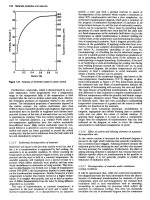
Circle drawing
The advantage
of
circle drawing is its symm-
etry. Once one
x,y
pair has been calculated, then eight points
on
the circle can be defined (Figure 5.27). Calculating the
plotted points using equal increments along the
x
axis is
Figure
5.24
Pixels plotting
using
integer division
Figure
5.25
Pixels plotted
using
nearest-pixel algorithm
unsatisfactory as shown in Figure 5.28. Better results are
obtained when points are plotted at equal angular rotations.
However, the calculation involves evaluating a
sine
and

cosine
function; trigonometric functions use a lot of CPU time. Some
means
of
reducing the number of trigonometric functions
which need
to
be evaluated is desirable.
Computer graphics systems
5/33
Figure
5.26
Bresenham’s line-drawing algorithm
Figure
5.27
ilsing the circle’s symmetry, eight points can be
plotted
for
each
(x,y)
coordinate pair
Polygon
method
If
the circle
is
drawn as a polygon, then only
a few calculations are required to determine the vertices after
which
a

straight-line algorithm is used to join the vertices.
sin(A
+
B)
=
sin(A)cos(B)
+
cos(A)sin(B)
sin(A
-
B)
=
sin(A)cosfB)
-
cos(A)sin(B)
cos(A
i
B)
=
cos(A)cos(B)
-
sin(A)sin(B)
cos(A
-
B)
=
cos(A)cos(B)
+
sin(A)sin(B)
For this polygon, the ‘radius’ is incremented by 2~/n radians

for
each of the
n
vertices.
If
the angle A represents the current
vertex, then the next vertex is found at an angle
of
A
+
2dn.
Instead
of
calculating the sine and cosine
of
this new angle, the
previous values
of
sine and cosine are incremented according
to
the expressions above. Thus:
sin(A
+
27h)
=
sin(A)cos(2~/n)
+
cos(A)sin(2~/n)
cos(A
i-

2dn)
=
cos(A)cos(2~/m)
-
sin(A)sin(2v/n)
Use
is
made of the following relationships:
Circle drawn
using
constant
x
increments
according
to:
y
=
fl
-x2
Figure
5.28
Circle plotted using equal increments along the x-axis
Now sin(A) and cos(A) become the new sine and cosine
values which will be updated for the next vertex. The two
multiplication operations and one addition operation per
function considerably reduce the computation required since
cos(2.rrln) and sin(2dn) only need to be calculated once. The
initial sine and cosine values can be selected to be
‘0’
and

‘1’
if
a full circle is to be drawn. Only the first 2~/8 radians need to
be calculated as shown above if one takes advantage of the
circle’s symmetry. This method
is
prone
to
cumulative errors,
but if these are less than half a pixel in total, then the method
is satisfactory.
Other curves
Functions in which the gradient
is
predictable
or
always less than unity (e.g. a circle) can always be plotted
by
incrementing in unit steps along one axis and calculating
the other coordinate. Complex curves may require the compu-
tation
of
the inverse function especially when the gradient is
large, if gaps in the curve are to he avoided. This is computa-
tionally expensive. Curve-fitting techniques and straight-line
approximations (e.g. polygon methods) considerably reduce
the computation required if the resulting accuracy is accept-
able.
Characters
Most applications require text

to
be displayed.
The most common form of manipulating text
is
to hold
bit-mapped
fonts
in memory, individual characters
of
which
are copied to the screen at the desired position. These
characters may be rotated in increments of
90”
by manipulat-
ing the matrix to allow vertical or inverted text. Different font
sizes may be produced by scaling the matrix although this only
gives acceptable results
for
a small range
of
font sizes. A better
solution is
to
hold each font in a variety
of
font
sizes.
The above techniques only permit text to be aligned
to
one

of
the axes.
For
text to be produced at any angle or orienta-
tion, matrix transformations are possible but do
not
give good
results. Using a
strokedfont
where characters are represented
by a small number
of
curves
(or
strokes) means that the
character definitions are independent
of
angle and also the
displayed size.
Most applications allow the user to define custom characters
or symbols.
In
this way, fonts containing other than Roman
characters may be used.
5/34
Computer-integrated engineering systems
Move and copy
Defined areas
of
the image can be quickly

and easily
copied
using BitBlt operations, thus avoiding repeti-
tion of previous calculations. This method is commonly used
to enter text from the font table to the display. However, not
all parts of the image can be
so
simply copied since overlapp-
ing blocks may be present.
In
this case the block will have to
be recalculated and redrawn at the new coordinates.
Move
operations require the steps above and, in addition, the
original block must be erased by recalculating and subtracting
from the frame buffer. Alternatively, to erase the image, a
rectangular area enclosing the image could be set to the
background colour (thus erasing overlapping blocks within the
area) and then any blocks partly defined in the area are
redrawn with windowing applied to reconstitute the image.
The options available in move and copy operations are
discussed in Section 5.3.4.3.
Area-fill
If
the shape of filled area is known, then the
operation employs a polygon-drawing algorithm using a plot
colour or pattern. When a pre-drawn area is to be filled, the
shape of the area may not be known
so
aflood-fill

algorithm is
required. To fill such an area with a colour or pattern, a closed
area is essential and a seed point within that area must be
supplied from which the fill will be determined. The fill
operation will set the pixels one row at a time within the
desired area until a boundary is reached. For example,
boundary may be defined as a foreground colour or the
background colour. Fill operations
on
areas containing pat-
terns give uncertain results if the pattern contains the bound-
ary colour. Most fill algorithms are recursive
so
that complex
areas may be filled. In such cases, the fill routine keeps a list of
start points for each line of pixels which are to be filled. When
it meets a boundary, it returns to the seed point and looks in
other directions where the fill might proceed.
Narrow areas of one or two pixels in width might prema-
turely terminate a fill operation. Since the fill proceeds one
row at a time, the narrow section might become blocked and
appear to be a vertex
of
the enclosed area, thus terminating
the fill. Section 5.3.4.3 describes some of the attributes of fill
operations.
Aliasing
Since pixels can only be drawn on a finite matrix,
continuous functions, when displayed, appear to have edges
which do not exist. This artifact is called

aliasing
and its effect
is to give diagonal lines a jagged appearance. In order to
reduce this effect, various means
of
anti-aliasing are
employed.
If
data in the frame buffer are processed to search
for edges some will be found to be true edges (Le. exist in the
real image) and can be ignored. Where aliasing is found to
occur the intensity of these and adjacent pixels can be mod-
ified to mask the edge. A form of Bresenham’s line algorithm
may be used to detect the relative position of a pixel from the
true line and the intensity is then set in inverse proportion.
Hardware techniques exist to reduce the ‘jaggies’ which
include pixel phasing and convolution operations.
Grids
A deliberate form of aliasing is used where the appli-
cation demands that all points be plotted on a grid or in an
orthogonal-only mode. For example, all pixel positions calcu-
lated by the application or entered by an input device which
fall within predefined areas are converted to the same pixel
position
-
that is, the centre
of
the defined area. The defined
areas depend on the grid spacing, which may be altered.
In

an orthogonal-only mode,
one coordinate from the
previously displayed point is fixed and only the other coor-
dinate is free to change (usually constrained to a grid).
5.3.4.3 Attributes of output primitives
Attributes may be defined for drawing opeiations which affect
line styles, colour and intensity. Line-style options include the
line width and pattern. The pattern may be a hatching pattern
in
one colour or a pattern using a number of colours. The
pattern will typically repeat every
8
or
16
pixels and may be
considered to be ‘tiled across the whole display. Only where
the line coincides with the tiled pattern are those pixels plotted
as part of the image. The most common line style is
solid.
Note that some attributes are not relevant or possible for
certain display devices. While the intensity of a line can be
varied for display on a CRT monitor, the same image will lose
intensity information when plotted
on
a monochrome laser
printer, for example. Referring to attributes individually, they
are called
unbundled.
When used in this way, the application
might require modification acccording to the display device

used. Similarly, colour information will not remain constant
when different displays are used, even for devices capable of
using colour. As an example, a CRT display normally draws in
white
on
a black background whereas a colour plotter would
draw in black on white paper; both would display a red line in
red. Thus attribute tables are often used which define the
foreground and background colours to be used when the
image is displayed on a CRT, to give one example. A whole
set of attributes may be defined for each display device, or
even for similar devices by different manufacturers. When
arranged in this fashion, they are given the name
bundled
atttributes.
Similar attributes are available to control fill styles.
When a block is moved or copied this may be combined with
a logical operation. For example, the source block may be
ANDed, ORed or Exclusive-ORed with destination and addi-
tion
or
subtraction operations may be set as attributes.
5.3.4.4 Two-dimensional transformations
Translation
This is a movement of a graphics object in a
straight line (Figure
5.29).
If the distance
(dw.
dy) is added to

each point in the object then the object will be translated
I
I
I
dx
‘I
v
Figure
5.29
Linear translation
of
an
object
Computer graphics
systems
5/35
linearly when redrawn. This is acceptable for lines or polygons
(which can be represented
as
a
set of lines). For circles and
arbitrary curves, the offset is applied to the reference point
(e.g. the centre
of
the circle) and the object redrawn.
Note that when an object
is
complex the redrawing of
translated objects can be quite slow. In an interactive mode
this can be

a
drawoack. Hence some applications do not
update the display completely except on request. This possibly
leaves some extraneous pixels set in the display but which are
cleared on the next display refresh operation. If BitBlt opera-
tions are not possible (due to overlapping objects, for
example) then some applications calculate
a
bounding box and
a
few reference marks on its edge in order to temporarily
describe the object. This
outline
image can be moved interact-
ively at high speed and the object is only fully redrawn when
the destination
is
fixcd.
Scaling
requires all relative distances of points within
an
object to be multiplied by
a
factor (Figure 5.30). This factor
is
usually the same for horizontal
and
vertical directions to retain
the proportions of the original object.
If

the scaling factor
differs in each direction, then the object will appear to be
stretched or compressed.
Figure
5.30
Scaling operation.
A
scale factor
of
2
is
applied to the
object relative to the
point
(x,y)
Rotation
requires multiplication
of
coordinates by sin0 and
cos@, where
0
is determined from the pivotal point. The new
coordinate is calculated from its position relative
to
the pivotal
point (Figure 5.31).
Reflection
produces an image which may be mirrored with
respect to the x-axis, y-axis or
a

user-defined axis (Figure
5.32). Changing the sign
of
one or both sets of world coor-
dinates will convert
a
point
so
that it is mirrored about one or
both orthogonal axes.
Shear
transformations can distort images (or correct for
perspective distortions) by making the transformation factor
a
function
of
the coordinate values (Figure 5.33).
Thus
the
transformation factor varies across an object.
\
rotate
Figure 5.31
Rotation
of
an object about the pivotal point
(x,y)
Matrix representations
All
of the transformations above can

be reduced to
a
sequence of basic operations, each
of
which
can be represented
as
a
3
x
3 matrix for
a
two-dimensional
display. For example,
a
linear translation
of an object by
a
distance
(dx,
dy) requires the coordinate
[x
y
I]
to
be
multiplied by the matrix:
Successive translations are additive such that two translations
of
(dx,

dy) and
(Sx,
Sy)
are equivalent to
a
translation of
(dx
+
Sx,
dy
+
Sy):
The
scaling
process requires more than one operation. The
first
translates
the object to the graphics origin. Thus the
second
(scaling)
operation can multiply all coordinates by the
same factor (Le. with respect to the origin). The final opera-
tion translates the object back to its original position. Thus
one scalar and two translation operations are required in the
following order:
100
mx
0
0
100

-dx
-dy
1
where
mx
and
my
are the scaling factors and
dx
and dy are the
distance of the object from the origin. These matrices may be
combined to give the scaling matrix:
0
The
rotation
process also requires translation to the origin
before the rotate operator
is
applied and the inverse transla-
tion
(as
above). The
rotation
matrix is:
5/36
Computer-integrated engineering systems
Figure
5.32
Reflection of an object about the x-axis
Figure

5.33
A
y-direction shear transformation on a unit square using a shear factor of
1
Computer graphics systems
5/37
where
0
is the angle
of
rotation. With the two translation
operations added, the overall matrix becomes:
cos8 sin8
-sin8 cos8
(1
-
cos@)&
+
dysin8
(1
-
cos8)dy
-
&sin0
1
Since all matrices can be multiplied together, then complex
transformations can be constructed by applying the matrix
operations in the desired order.
5.3.4.5
Windowing and clipping

Windowing
A
window
is
a rectangular display area. There is
normally a single window displayed which occupies the whole
screen. However, it
is
now common to find software which
uses windows freely and there may be several windows
displayed at once. An architecture which allows only a single
process to run at any one time may display multiple windows,
but only one can be an
active
window. Multi-tasking
or
multi-processor systems may have several windows which are
active, i.e. each is controlled by a different
process
which is
running.
Where multiple windows are displayed they will often
overlap
so
that the window which has lower precedence
(or
is
a
background
window) is partially or totally obscured (Figure

5.34). Hardware techniques are available to manage such
overlaps, but more commonly this is performed in software.
Clipping
operations are performed when the contents of
a
window are being displayed
so
that only pixels within the
permitted window limits are drawn; pixels outside the window
area are
clipped
(Figure 5.35). The window boundaries and
attributes are defined in a higher layer
of
the software
-
the
window manager,
which
is
conceptually part
of
the operating
system. The window manager may draw a border around the
window itself and label the border appropriately, but this is
transparent to the process using the window. It is possible
to
define the windowing operation in terms of world or display
coordinates (see Section 5.3.4.1) and ‘window’ is often used
interchangeably when referring to either coordinate system.

Where a distinction needs to be made between the two, the
term
viewpoint
refers
to
the rectangular area on the display
device.
3
Figure
5.34
Multiple
overlapping windows
I
I
Figure
5.35
Clipped
graphics
The most common operations to be performed on a window
are described below and are implemented by calls to the
window manager.
Create
The dimensions and position of ?he new window
are given and a
handle
is returned if the window is
successfully created. This handle is used in future graphics
calls
to
specify the window in which drawing operations

are to take place.
A
newly created window will normally
have the highest priority
so
that it may obscure parts of
existing windows.
Clear and delete (close)
The window handle
is
used to
specify the window to be cleared or closed.
It
may not be
possible
to
close a window if ?he process which owns
it
is
still active.
Drag (move)
The size and contents
of
the window are
unchanged, but the position in the display
is
altered
(Figure 5.36).
A
translation operation is used to perform

this. The window position is normally constrained
so
that
no part may be dragged off the display, otherwise further
clipping may become necessary.
Resize
The dimensions
of
the window are changed by
altering the clipping parameters. The contents of the
window which are visible before and after
this
operation
remain unchanged (Figure 5.37).
5/38
Computer-integrated engineering
systems
Figure
5.36
Dragging
a
window
5.
Zoom
The contents of the window are recalculated
using a new scaling factor (Figure
5.38).
6.
Pan
Here, the

viewport
is unchanged in position and
size, but the window moves ‘behind’ the viewpoint. This is
a translation operation but the clipping attributes do not
‘move’ with the window (as for
drag)
but rather remain
constant as far as the display coordinates are concerned
(Figure
5.39).
Priority
A
window can be brough to the foreground or
sent to the background by assigning it the highest or
lowest priority attribute. If an intermediate priority is
assigned, then the window may obscure parts of some
windows and may itself be partly obscured by other
windows (Figure
5.40).
7.
Clipping text
Where the clipped object comprises text, then
clipping at the window boundary can leave partial characters
visible in the same way as graphics objects are clipped at the
pixel level. Sometimes this is visually undesirable. Thus text
may be treated differently such that if any part
of
a character
would be clipped, then that character is not displayed (Figure
5.41).

Updating the display
When an operation takes place which
disturbs the boundaries
of
the viewpoint then it is not only the
4
window itself which needs to be redrawn; any part
of
the
display which was partially obscured by the old viewport will
also need to be redrawn (Figure
5.42).
If the background is now visible, the revealed areas are
simply cleared to the background colour.
If
parts of other
windows are revealed then two strategies exist. Either the
whole window is redrawn and the window manager clips the
pixels according to the window’s priority, or an ‘intelligent’
process will only redraw those parts of the image that had
previously been obscured. The first strategy is the simplest,
but has the disadvantage of redrawing even those parts
of
the
image that are correctly displayed
-
which means that overall
system performance suffers. The second strategy is the most
efficient in that only the area which requires redrawing is
changed. This requires that the process itself can determine

which objects or parts of objects were obscured and then
require redrawing. This is not always easy to do or to
calculate.
If
the windowing is performed in hardware, then the display
buffers do
not
become corrupted where windows overlap as
each window has its unique, non-overlapping buffer. Thus
when moving a window reveals another,
no
redrawing of the
image buffer is required. The display hardware fetches data
from the appropriate buffer as each window or part thereof is
displayed
on
the output device.
5.3.4.6
Segments
Graphics objects may sometimes be repeated within an image.
it is wasteful to store the same information several times
so
such objects may be stored as subpictures or
segments.
These
objects are not restricted to being identically portrayed in the
output image since variations of the same object can be
produced by changing the attributes
of
the object.

A
related hardware technique involves the use of
sprites.
In
this way a graphics object can be predefined and held in
memory. Whenever this object is required, it can be quickly
copied into the frame buffer at the required position without
requiring graphics processing operations to draw it. However,
there is usually the restriction that attributes cannot be
changed and
so
the sprite is fixed in size and colour.
Figure
5.37
Resizing
a
window
Computer
graphics
systems
5139
he selected win
Figure
5.38
Zoom
operation on a window
i
Figure
5.39
Pan

operatlon
on
a
window
Original
display
s
shown within
1
Window
2
to
foreground
Figure
5.40
Changing the priority
of
window
2
5/40
Computer-integrated engineering
systems
usually undesirable
characters to be dis
In this case, any ch
which would be part
are not displayed.
When
text
is

clipped:
it
is
=for partial
characters to be disglayed.
In this case, any chqracters
c
are
- -
-
not
-
- -
djqlgygj,
-
1
hich
would be partially delete
Figure
5.41
Clipped text
Figure
5.42
When a window
is
moved, the area exposed
must
be
redrawn
5.3.5

Workstations
Workstation configurations vary from a single personal com-
puter with its own screen, through a host computer with a
graphics coprocessor using a separate screen, to a high-
resolution multi-processor system incorporating many input
and output devices.
5.3.5.1 Integrated workstations
This describes the standard ‘personal computer’ configuration
where the processor runs the application, and the graphics
hardware and the screen are contained in essentially one unit.
Coprocessors may be used to accelerate certain operations,
but they are under the control of the main processor. The
processor itself is likely to he a fast 32-bit device with memory
management. It will also allow multi-tasking and support
multiple windows.
Area
to
be
redrawn
5.3.5.2
Hostislave configuration
In this case, the host computer provides mass storage, key-
hoard entry and interfaces for printers and plotters. The slave
graphics processing unit contains the frame buffer, drawing
and display hardware and is semi-autonomous. The two units
are linked by a bus. In this way, the host runs the high-level
application software and produces a display list to the slave.
The slave is optimized to interpret the display list and perform
the drawing operations at high speed.
The two parts

of
the system partition the process into high-
and low-level operations and can work in parallel for much of
the time.
5.3.5.3 Operating systems
Many PC-based systems use
MS-DOS
or some form
of
display
manager. Only ‘386 systems and later allow true multi-tasking.
The virtue of such a system is that it is multi-purpose and can
Computer graphics systems
5/41
provide a system for both word processing and graphics
processing, it is therefore cost-effective.
UN1X"-based systems are multi-tasking and usually multi-
user as well, although only a limited number of high-resolution
terminals are allowed per node before the system performance
suffers. UNIX allows several input and output devices to be
added
to
the system and accessed by various users. Portability
of
applications between UNIX systems
of
different manufac-
ture is a strong advantage. UNIX systems may range from a
desk-top computer
to

a large main-frame installation.
VMSi.
systems based around the VAX architecture are not
generally as portable
to
third-party hardware. However, VAX
installations are fairly common for this not to be a severe
drawback. A large resource
of
VMS-based graphics software
is available.
An
increasingly common feature is
networking,
where a
number
of
high-performance graphics workstations are net-
worked together
to
share central resources (or distributed
resources). Since each workstation has its own processor
(or
processors) other users
of
the network are not disadvantaged
when
one
user initiates some computing-intensive task. Only
when simultaneous access is made by two workstations to a

shared resource (e.g.
a
fileserver) is any drop in performance
apparent.
5
e
3
a
6
~~~~ee-~~~ension~l
concepts
Three-dimensional concepts and operations are simply an
extension of the two-dimensional concepts described in Sec-
tion 5.3.3.4. For display purposes
on
two-dimensional devices
further transformations must take place to give a three-
dimensional
representation
in two dimensions.
5.3.6.1
Introduction
The coordinate system used is normally three orthogonally
related axes:
x,
y
and z. Translation, scaling, rotation reflec-
tion and shear operations are performed in a similar manner
to
the two-dimensional operations but for three dimensions. For

example, .the
linear
translation
of
an object by a distance
(dx,
dy, dz) requires the coordinate
[x
y
z
11
to be multiplied by the
matrix:
Original
Object
Figure
5.43
Perspective projection
Compare this with the two-dimensional linear translation
metsix 2nd observe the similarity:
More three-dimensional transformations are given in Section
5.3.6.4.
5.3.6.2
Three-dimensional display techniques
A three-dimensional object will
be
projected
onto
a two-
dimensional plane for display.

If
the z-axis
is
arranged
to
be
normai
to
the plane
of
the display then no transformation of
*
UNIX
is
a Trademark
of
AT&T
Bell
Laboratories,
Inc.
t
VMS
is
a
Trademark
of
the Digital Equipment Corporation
Figure
5.44
Two views

of
an office from different viewpoints
(courtesy
of
AutoCAD)
5/42
Computer-integrated engineering
systems
the
x
and
y
planes is required. However, depth information
can be represented by allowing the
z
distance to offset the
x
and
y
coordinates by an amount proportional to the distance
from the front
of
the object. This results in
aparallelprojection
onto the viewing surface (flat perspective).
For a more realistic
perspective projection,
the depth-
modified coordinates are calculated from the distance of a
point from the Centre

of
Projection. Thus distant objects
appear smaller, as shown in Figure
5.43.
5.3.6.3
Three-dimensional representations
It is not always desirable to view an object along the z-axis as
described above. Any arbitrary
viewing point
could be chosen
so
that views from any point around an object and from any
distance could be chosen (Figure
5.44).
Indeed, the viewing
point may be inside an object, giving an internal view. The
projection onto the display plane requires the translation,
scaling and rotation operations described in Section
5.3.6.4.
If all points in an object are translated from the three-
dimensional object onto the viewing plane, then a
wire-frame
drawing results (Figure
5.45).
This is acceptable as a represen-
tation, but is not realistic. In a solid object, many points are
hidden from view by parts
of
the object itself. The image can
be processed to determine which points would normally be

hidden from the chosen viewpoint and these points are not
plotted (Figure
5.46).
This process is called
hidden-line
removal.
Figure 5.45
Wire-frame drawing (courtesy
of
AutoCAD)
Shading
Once hidden line removal has been performed, the
object appears solid. A better impression
of
depth can be
given if the facets or surfaces are
shaded.
This implies that an
imaginary light source
is
introduced into the model. Those
surfaces at an angle which would reflect light from the light
source to the viewpoint appear bright, and as surfaces differ
from this angle,
so
their intensity is reduced. The facets are
still clearly visible at this point.
In
order to model a smoothly
curved surface some form of intensity interpolation is

employed, the most common being
Gouraud shading.
This idea can be extended to model
shadows
for a high
degree of realism and to perform
ray-tracing
so
that the effect
of
transparent and refracting objects can be represented
(Figure
5.47).
Figure 5.46
Figure
5.45
with
hidden-line elimination (courtesy
of
AutoCAD)
Shading itself can be performed in a number
of
ways.
Dithering
retains a fixed pixel size and density but groups
pixels into
superpixels
which may contain
2
X

2,
3
x
3
or
larger arrays. This is also called
half-toning.
A
2
x
2
array
may represent five grey levels according to the number of
pixels set in the superpixel
(0
to
4),
but the resolution is halved
in this example.
Continuous tone
is used to give ‘photographic’
quality since the density
of
a pixel may be varied over a
continuous range from black to white. The final displayed
resolution is not affected by this process.
5.3.6.4
Three-dimensional transformations
The transformation mentioned in Section
5.3.6.1

can be
reduced to a sequence
of
basic operations, each of which can
be represented as a
4
x
4
matrix. Only the basic operations
are described here.
Figure 5.47
Ray-traced image (Acorn Archimedes computer,
software
by
Beebug)
Computer graphics
systems
5/43
The
linear translation
of an object by
a
distance
(dx,
dy, dz)
requires the coordinate
[x
y
z
11

to
be multiplied by the matrix:
The
scaling
process requires more than one operation. The
first
translates
the object
to
the graphics origin. The second
scaling
operation can scale all coordinates by the scaling factor
with respect
to
the origin. The final operation translates the
object back to its original position. The scaling matrix
is:
mx
0
0
0
omyo0
0
0
rnz0
0
0
01
where
~JC.

my
and mz are the scaling factors in each dimen-
sion. If
dx,
dy and dz are the distances of the object from the
origin in each dimension, then the combined scaling operation
with translation becomes:
mx
0
0
0
0
rny
0
0
0
0
rnz
0
(1
-
mx)d.~
(1
-
my)dy
(1
-
mz)dz
1
The

rotation
process also requires translation to the origin
before the rotate operator and the inverse translation are
applied (as above). In the three-dimensional case, the axis
of
rotation is arbitrary and
is
not necessarily aligned to any
of
the
three axes. Taking the simple case where
a
z
axis rotation
is
performed, the
rotation
matrix
is:
cos0
sin0
0 0
-sin8 cos0
0
0
0
0
10
0
0

01
where
0
is
the
angle
of
rotation. It can be seen that this is
similar to the two-dimensional case.
~~~n~w~i~dge~e~~
Dr
D.
N.
Fenner, King's College, London (Figures 5.20 and
5.21).
resenham's
line
algorithm
In Figure 5.26 the line
is
assumed to have
a
slope
of
less than
1.
The straight line
is
plotted for constant
x

increments which
are equal
to
the
x
pixel increment. Thus the position
x,
is an
integral pixel coordinate and the distance
x,
-
x,+1
is equal to
the
x
pixel increment.
In
order to plot the line, the equivalent
y
pixel positions must be found for each
x
pixel coordinate.
The real
y
coordinate is given by:
yn
=
mx,
+
b

This will normally not fall onto an integer pixel position
so
the
nearest
y
pixel must be found.
In Figure 5.26 the distance
of
the point
(x,,
y,)
from the
neighbouring
y
pixel positions
(PI
and
P2)
are shown to be
dl
and
dl.
The smaller
of
dl
or
d2
is
used to select the pixel to be
plotted. These distances are caicalated

as
follows:
(5.1)
dl
=
Yl
-
Yn
d2
=
Yn
-
Y2
=
yl
-
mx,
-
b
=
mx,,
+
qb
-
y2
(5.3)
The difference
dl
-
d2

is calculated. If the result is positive,
then the line is closer to
P2.
If
the result is negative, the line is
closer to
PI.
Now,
dl
-
d2
=
yl
+
y2
-
2mx,
-
26
(5.4)
Here,
y2
=
y1
-
1
since
yl
and
y2

are integer pixel coordinates
which simplifies equation
(5.4),
as
shown later.
Once the start of the line has been calculated and the
nearest pixel found. it is not necessary to calculate
y
=
mx
f
b
each time and then calculate the nearest
jj
pixel
position. Instead, a constant
(Ay)
is
added
to
the previous real
y
value for each increment
of
Ax
along the
x
axis, where
Ax
is

the
x
pixel increment and
Ay
=
mdx.
Substituting for
y2
in equation (5.4) and multiplying by
Ax
gives:
(d,
-
d2)AX
=
2dXy1
-
~AYx,
-
(2b
+
l)Ax
(5.5)
The left-hand side of the expression is positive
if
the he is
closer
to
P2
or negative if closer to

P1.
It
is
possible
to
calculate
the new lhs
of
the expression from the previous one as shown
below, where the lhs is denoted
0,.
The final term in equation
(5.5) is
a
constant term, therefore:
W,
=
2Axy1
-
~AYx,,
-
c
where
c
=
Ax(2b
+
1)
and
@,+I

=
AXY YO
-
2dyxnL1
-
c
Therefore
w,+~
may be derived from
w,
since
@,+I
-
W,
=
2Axbo
-
y1)
-
2Ay
since
x,+~
=
x,
+
1.
Thereafter,
w,+~
is evaluated using
For the first point in

a
line,
w1
is
calculated from
2Ay
-
Ax.
(5.6)
a,+,
=
W,
+
2Axbo
-
y1)
-
2A)l
The sign of this expression determines whether the upper or
lower pixel is plotted.
It can be seen that multiplication by an integer and addition
and subtraction operations are required, and these operations
are easily performed by digital processors.
References
1
2
Tanenbaum,
Structured Computer Organisation,
Prentice-Hall,
Englewood Cliffs,

NJ
(1984)
IGESIPDES Organization
(PO)
-
Committee: IS0
TC
184ISCIIWGI and WG2 ref.: NCGA,
PO
Box 3412. McClean,
Virginia,
USA
Further reading
Angel,
E
Computer Graphics,
Addison-Wesley, Reading.
MA
Arthur
(ed.),
CADCAM: Training and Education through
the
'80s
Berk,
Computer Aided Design and Analysis
for
Engineers,
Bertoline,
Fundamentals
of

CAD,
Delmar Publishing Inc.
(1985)
Bielig-Schulz,
G.
and
Shulz,
C
30
Graphics in Pascal,
Wiley.
Chichester (1989)
Blauth
and
Machover,
The
CAD/CAM Handbook,
Computervision
Corporation, Bedford,
MA
(1980)
Bono,
P.,
Encarnacao,
J.
L.,
Encarnacao,
L.
M.
and Herzner,

W.
R.;
PC
Graphics with
CKS,
Prentice-Hall, Englewood Cliffs,
NJ
(1990)
(1990)
(Proceedings
of
CAD
ED
'84),
Kogan Page, London (1985)
Blackwell Scientific, Oxford (1988)
5/44
Computer-integrated engineering
systems
Bowman and Bowman,
Understanding CAD/CAM,
Howard Sams
and Co., Indianapolis (1987)
Boyd, A,,
Techniques
of
Interactive Computer Graphics,
Chartwell-Bratt, Bromley (1985)
Bresenham,
J.

E., ‘Algorithm for computer control of digital
plotter’,
IBM Systems Journal,
4,
25-30 (1965)
Burger, P. and Gillies,
D.,
Interactive Computer Graphics,
Addison-Wesley, Reading, MA (1989)
Chang and Wysk,
An introduction to Automated Process Planning
Systems,
Prentice-Hall, Englewood Cliffs, NJ (1985)
Earnshaw, Parslow and Woodwark,
Geometric Modelling and
Computer Graphics, techniques and applications,
Gower
Technical
Press,
Aldershot (1987)
Farin,
Curves and Surfaces for Computer-Aided Geometric
Design
-
A
Practical Guide,
Academic Press, San Diego (1988)
Foley, J.
D.,
van

Dam, A., Feiner,
S.
K.
and Hughes,
J.
F.,
Computer Graphics,
2nd edn, Addison-Wesley, Reading, MA
(1990)
Gerlach,
Transition to CADD,
McGraw-Hill, New York (1987)
Groover and Zimmers,
CADICAM: Computer Aided Design and
Manufacturmg,
Prentice-Hall, Englewood Cliffs, NJ (1984)
Haigh,
An Introduction to Computer Aided Design and
Manufacture,
Blackwell Scientific, Oxford (1985)
Hawkes,
The CADCAM Process,
Pitman, London (1988)
Hearn,
D.
and Baker, M. P.,
Computer Graphics,
Prentice-Hall,
Englewood Cliffs, NJ (1986)
Hewitt,

T.,
Howard,
T.,
Hubbold, R. and Wyrwas,
K.,
A
Practical
Introduction to PHIGS,
Addison-Wesley, Reading, MA (1990)
Hoffmann,
Geometric and Solid Modelling
-
An Introduction,
Morgan Kaufmann, San Mateo, CA (1989)
Ingham,
CAD Systems in Mechanical and Production Engineering,
Heinemann Newnes, Oxford (1989)
Kingslake, R.,
An Introductory Course in Computer Graphics,
Chartwell-Bratt, Bromley (1986)
Laflin,
S.,
Two-Dimensional Computer Graphics,
Chartwell-Bratt,
Bromley (1987)
Machover,
The C4 Handbook
-
CAD CAM CAE CIM.
Tab

Books, PA (1989)
Mair, G. M.,
Industrial Robotics,
Prentice-Hall International
(UK)
Ltd (1988)
Majchvzak, Chang
et al., Human Aspects of Computer Aided
Port,
Computer Aided Design for Construction,
Collins, London
Rooney and Steadman,
Principles of Computer Aided Design,
Voisinet,
Introduction to CAD,
McGraw-Hill, New York (1986)
Design,
Taylor
&
Francis, London (1987)
(1984)
PitmaniOpen University (1987)
6
Design standards
I.
L
Jlnll"nl"lLClll"ll
111
"Gxg,,
OlJ

0.3
Ergonomic ana anrnropomerric data
6/23
6.1.1
Introduction
6/3
6.12
Modular design
6/3
6.6
Total quality
-
a company culture
6/29
Machine details
6/
Design procedure
6.1.7
6.1.8
6.2.1
Drawing references
6/4
6.2.2
Preferred sizes
Levels
of
stand
Management and organization
o
information

615
6.2.3
Microfilm and computer technologies
j.3
Fits, tolerances and limits
6/7
6.3.1
Conditions
of
fit
6/7
6.3.2
Definition
of
terms
6/7
6.3.3
Selecting fits
6/13
6.3.4
Tolerance and dimensioning
6/13
6.3.5
Surface condition and tolerance
6/14
i.4
Fasteners
6/14
6.4.1
6.4.2

6.4.3
6.4.4
6.4.5
6.4.6
6.4.7
6.4.8
6.4.9
6.4.10
6.4.11
6.4.12
6.4.13
6.4.14
6.4.15
6.4.16
Automatic insertion
of
fasteners
6/15
Joining
by
part-punching
6/17
Threaded fasteners
6/17
Load sensing in bolts
6/17
Threadlocking
6/19
Threaded inserts and studs
for

plastics
6/20
Ultrasonic welding
6/20
Adhesive assembly
6/20
Self-tapping screws
6/20
Stiff nuts
6/21
Washers
6/21
Spring-steel fasteners
6/21
Plastics fasteners
6/21
Self-sealing fasteners
6/21
Rivets
6/21
Suppliers
of
fasteners
6/21

Standardization
in
design
613
6.1.4

Levels of standardization
Standardization can operate at different levels: company,
group. national, international, worldwide.
It
can be applied to
many aspects
of
the activities
of
design and manufacture, e.g.
terminology and communication, dimensions and sizes, testing
and analysis, performance and quality. It is a broad-ranging
subject and standardization will be exemplified below
in
further detail but only in
so
far as it serves the design function.
The descriptions are drawn largely from experience with
British Standards,
but
at the time
of
writing
(1988)
consider-
able efforts are continuing to harmonize
BSI
activities with
European counterparts. Indeed, many British standards are
entirely compatible with

IS0
standards and are listed as such
in the BSI Catalogue which is published annually.
6.1
Standardization
in
design
6.1.1
Introduction
Standardization in design is the activity
of
applying known
technology and accepted techniques in the generation of new
products. This may be interpreted as almost a contradiction in
terms: if something
ns
standard then there is little left to
design. On the other hand, if standardization is seen as a
means
to
promote communication in design and manufacture
then its usefulness is clearer: time is
not
wasted in redesigning
the wheel. Again, if standardization
is
seen as providing
targets that products must attain then we have criteria for
acceptance in performance and quality: you know what you
are getting.

These points illustrate the difficulty in understanding the
role
of
standardization within industry at large, and why
it
is
too
often ignored by designers and management. One does
not
want
bo
be constrained. In fact, the converse is usually
true, that by adopting standards in an appropriate manner, the
designer is freed from niany detail decisions that would
otherwise hinder the overall scheme.
It
has to be acknow-
ledged that some standards are inherently retrospective. That
is.
a standardized design method or procedure is bound to be
based
on
past practice. and in some circumstances this may
inhibit flexibility in adopting new methods. But
to
counteract
this, the designer may well contribute to updating and dev-
elopment
of
new standards. Indeed, the standards organiza-

tions have deveiopmext groups and committee structures for
this very purpose.
4.
P
.2
Modular design
Standardization in design may be applied by the idea of
modulariization. That is, a range
of
products
of
related type or
size may be designed
(or
redesigned)
so
that complex
assemblies may be made up from a few simple elements
or
modules For example.
a
vast range
of
electric motors and
gearboxes can be made from a few each of motors, bases,
flanges, gear cases, gears, shafts and extensions.
This approach applies particularly well to complex, low-
volume production
of
products where each customer wants his

or her own version
or
specification. The economics of indi-
vidually designing for each customer would be prohibitive but
the desigr. of a few well-chosen modules would cover the
majority
of
requirements. Other examples where modular
design may be applied are: overhead travelling cranes, water
turbines, hydraulic cylinders. machine tools (BS 3884: 1974).
6.1.3
Preferred
sizes
Related
to
the modular design concept is the idea
of
preferred
sizes.
In
any range
of
products there is usually some character-
istic feature such as size, capacity, speed, power. It is observ-
able that an appropriate series of numbers can cover a large
proportion of requirements.
For
many practical situations the
geometric series known as the Renard Series may be used (BS
2045:

191%
=
IS0
3). The key point in application is the
product-characteristic feature
to
which the Series is applied.
Tnis application
of
standardization is one
of
the best ways
of
promoting economy in manufacture by variety reduction. it
also
faciliiates manufacture by sub-contracting and eases the
problems
of
spares availability for maintenance.
A
further
discussion is given in reference 3.
6.1.5
Machine details
Standard proportions are laid down and specified precisely
with dimensions and preferred sizes. This is the most obvious
use of standardization in design and is employed widely,
almost without conscious effort.
6.1.5.1
Examples

BS 3692: 1967 Metric nuts bolts and screws (IS0 4759)
BS
1486: 1982 Lubricating nipples
BS 4235: 1986 Parallel and taper keys for shafts
(IS0
774)
BS 6267: 1981 Rolling bearing boundary dimensions
(IS0
15)
(also
BS
292: 1982 for more detailed dimensionai specifica-
tions)
BS
1399: 1972 Seals, rotary shaft, lip. Shaft and housing
dimensions
BS
3790: 1981 Belts
-
vee section. Dimensions and rating
(IS0
155)
BS
11:
Railway rails
(IS0
5003)
6.1.6
Design procedure
A procedure, algorithm or method is described

for
application
in circumstances where long experience has established satis-
factory results. This is often very useful to the designer as a
starting point but evolution beyond the standards is very
probable in particular industries. Such standards are among
those most iikely to be influenced and developed by designers
themselves. They may. however, be adopted
as
part
of
a
commercial contract and thereby promote confidence in safety
and reliability.
6.
I.
6.1
Examples
BS 436: 1986 Spur gears, power capacity
(IS0
6336)
BS
545: 1982 Bevel gears, power capacity (IS0 677. 678)
BS
721: 1983 Worm gears, power capacity
(note the recent revisions
of
these very well-established stan-
dards)
BS

2573: 1983 Stresses in crane structures
(IS0
4301)
BS
1726: 1964 Helical coil springs
BS
4687: 1984 Roller chain drives
(IS0
1275)
BS 1134: 1972 Surface finish
(IS0
458)
BS
5078: 1974 Jigs and fixtures
BS
5500: 1985 Unfired welded pressure vessels
(IS0
2694)
4.1.7
Codes
of
practice
Methods for design, manufacture and testing are recom-
mended in these types
of
standard, and, like ‘design proced-
ures’ described above, they may form the
basis
of
a comrner-

614
Design standards
cia1 contract. Again, they are codes that may or may not be
followed entirely but may be regarded as facilitating effective
communication between vendor and purchaser or any other
interested parties.
6.1.7.1
Design: Examples
BS 5070: 1974 Graphical symbols and diagrams
BS
308: Part
1:
1984 Engineering drawing practice (IS0 128):
BS 308: Part 2: 1985 Dimensioning
(IS0
129) (see also
reference 1)
BS 4500: 1969 Limits and fits (IS0 286)
BS 5000: Part 10: 1978 Induction motors (CENELEC HD231)
BS Au 154: 1989 Hydraulic trolley jacks
BS CP117: Part 1: 1965 Simply supported beams
BS 4618: 1970 Presentation of plastics design data
6.1.7.2
Manufacture: Examples
BS 1134: 1972 Surface texture assessment (IS0 468)
BS 5078: 1974 Jig and fixture components
BS 5750: 1987 Quality assurance system (IS0 9000) (see also
reference 2)
BS 970: 1983 Steel material composition (IS0 683)
BS 6323: Parts 1-4 Steel tubes, seamless

BS 4656: Parts 1-34 Accuracy of machine tools (IS0 various)
(e.g. Part 34: 1985 Power presses
=
IS0 6899)
BS 4437: 1969 Hardenability test (Jominy) (IS0 642)
BS 6679: 1985 Injection moulding machine safety (EN 201)
6.1.8
Abbreviations used
BS British Standard
BSI British Standards Institution
Au Automobile Series (BS)
IS0 International Standards Organization
EN European Normalen
CP Code of Practice
Notes: 1. Some standards are divided into separately pub-
lished parts. Details are given in the BS Catalogue.
2. Many colleges, polytechnics, universities and
public libraries hold sets of standards.
A
list is
given in the BS Catalogue.
6.2
Drawing and graphic communications
Since the days of cave dwellers, drawings have been a prime
means of communications and today, with all the latest hi-tech
innovations, drawings and graphics still hold a pre-eminent
position. The needs are the same
-
all that has changed is the
methods by which drawings are made, stored, retrieved and

used. Never was a saying more true than ‘One picture is worth
a thousand words’.
In the world
of
engineering, drawings are absolutely essen-
tial. They may first be sketches arising from customers’ needs
or competitive designs but. from several sources, ideas can be
given a form around which discussions can take place as to the
idea’s marketability, usefulness, etc. From this point, a com-
ponent design starts to emerge. It will undergo many changes
to satisfy the demands
of
various departments, e.g. produc-
tion, servicing. installation, stress analysis, marketing, etc. All
these changes will be documented, particularly if the company
is adhering to the BS 5750 quality assurance code.
Because we see in a three-dimensional way, perspective and
isometric three-dimensional drawings always provide a
quicker appreciation
of
a design than the more familiar plans
and elevations. Perspective and isometric drawings are,
however, more difficult and time consuming to produce,
require special skills and do not lend themselves to dimension-
ing. Thus the communication of an idea to the shopfloor for
manufacture has generally been through the medium of plans
and elevations of the item.
In preparing such drawings, dimensions should always be
taken from datum lines which, ideally, should be coincident
with the hardware itself rather than being a mere line in space.

Using such a datum as a reference avoids a dimensional
build-up
of
accumulated errors.
In the late nineteenth and early twentieth centuries, when
life progressed at a more leisurely pace, engineering drawings
and architectural plans were often works of art. Parts were
shaded and coloured. This practice died out in the 1920s,
although even today many architects’ drawings not only use
shading and colour but widely employ isometrics and perspect-
ives. However, the audience for these drawings is rather
different to that viewing engineering drawings. Architects’
ideas and proposals are largely for public consumption and
will be read by lay people as well as by builders and other
planners. The public are often bemused by plans and eleva-
tions, particularly when some practices use third-angle projec-
tion and others first-angle projection.
Engineering drawings are mainly read by craftsmen who
are, however, well trained in reading such drawings.
A
notable exception was during the Second World War, when
many engineering companies found it necessary to include
isometric or perspective drawings
on
the plans to give a visual
appreciation of the part in question to the wartime workers
on
the shopfloor, many of whom had
no
knowledge or training of

either mechanical engineering or drawings.
While a drawing will detail the geometry of a part and its
method of assembly it cannot define graphically such things as
finish, smoothness or material, although there are standard
symbols which give a measure of surface roughness. Neverthe-
less, for these, annotations are required. Text and tables are
often included
on
drawings and, together with drawn lines,
complete a total engineering drawing.
Design is essentially a ‘doing’ activity and design skills
develop through practice. Design learning needs a structured
approach aimed at building up confidence and competence
with definite educational objectives at each phase. Much of
the first year at college is spent
on
learning drawing skills such
as orthographic projection, sketching, tolerances and as-
sembly drawings. These are essential for later work, and much
emphasis is placed on the fact that drawings are the medium
used by engineers
to
communicate ideas.
Ideally, a drawing should transmit from one person to
another every aspect
of
the part
-
not only its shape but also
what is is for and how it should be made and assembled.

6.2.1
Drawing references
Not the least important aspect is how the parts are referenced.
It may seem a simple enough task to apply a number to a
drawing or part and listing it in a register, but subsequent
identification may prove more of a problem. Therefore speci-
fic numbering systems are introduced. Depending on the
users’ requirements, systems can be simple or complicated.
For instance, every drawing of a part belonging to one
complete assembly may be given a prefix, either character or
number (for example, A/1234, where A defines the particular
assembly and 1234 the individual part). This means that if a
spare is required, the first sort (A) in the drawing register
Drawing and graphic communications
6/5
complexity, depending on the range of products. whether, for
example, they are aircraft or Iawnmowers. However, each
company must have fac es for conceiving
a
design and
developing and then producing it. The prime task of engin-
eering management is to create and sustain such an organiza-
tion and direct it to the achievement of the declared objective.
Behavioural science focuses attention on the nature of
individual and group interaction in an organization; that
is.
how people can work together in harmony. It emphasizes
people rather than jobs. and underlines the simple truth that
every organization must solve the problem
of

relationships
among its staff
if
an efficient working environment is to be
realized. Argysis' has stated:
The individual and the organization are living organisms
each with its own strategy for survival and growth. The
individual's strategy for existence is. at crucial points,
antagonistic to the strategy that guides the formal organiza-
tion. This may lead
to
continual conflict between the
individual and the organization. The conflict, however can
be a source for growth as well as a stimulant for disintegra-
tion.
Management has to solve problems within the context
of
the
organization. The individual cannot usually work without a
relevant organization structure, and the organization, in turn,
depends almost entirely on the individual. However. their
interests differ, and the manager's job is
to
develop a properly
balanced interaction of individual needs and organizational
demands.
Engineering design
is
a corporate activity, involving teams
of

people whose job it is to provide a prescription
of
what is to
be produced. How people interact can be determined by the
shape of the organization.
The resources of design are not like production facilities. In
a
machine shop it is possible to programme work for optimum
utilization in accordance with machine capabilities. Designers,
however, cannot be
so
programmed and their performance,
for many valid reasons, is often unpredictable. Nevertheless, a
design organization is expensive, and it is essential to study its
function in the same way as machine fmctions.
In
design and development organizations a careful balance
between order and flexibility has to be obtained. Should. for
example. a design office be centralized for several production
groups or decentralized? Where there
is
little change. formal
policies, procedures and rules to obviate communication diffi-
culties and aid designers would be preferable. Where change
is
more or less continuous, a more dynamic grouping or task
forces may work better in relation
to
specific
jobs.

Over the years: considerable research has been undertaken
(1)
to find out what information designers want and how it
should be best presented and
(2)
to develop convenient
methods by which relevant information and data can be
transferred to others. Several universities, polytechnics and
colleges have been involved in this particular work and, since
1971, the Design Group at Southampton University have set
up a series
of
seminars to discuss these various activities.
During the
1960s
a
number
of
commercial systems were
devised to provide designers with product data. Most fell by
the wayside over the years although one, TI Index. not only
survived but has been developed
to
take advantage of today's
technology in microfilm and computer-aided storage and
retrieval.
defines a particular assembly while the number will locate the
individual part. This can be developed further by taking, say,
the first two digits
of

the number
1234
(Le. 12) and stating that
all parts bearing the first two digits are made from flat metal
sheet as distinct from, say,
13
for castings, 14 for plastics parts
and
so
on. The original part AD234 would thus be defined as
belonging to
a
particular assembly (A) and would be seen as a
part made from flat metal sheet
(12)
with the individual part
number
of
34.
This can be further enhanced (or complicated)
by the addition of a modification number
or
character which
introduced the part or represents the year of manufacture
and/or a part modified in shape or dimension. The whole
purpose
of
the system is to locate the part number and/or its
drawing from a part in service which may be damaged or
overpainted. eliminating the part number.

Spares lists often carry exploded drawings in which a
particular assembly is shown as a set of parts approximating in
position to the assembled location. Ali these ploys help to
identify any particular part whose title (for example, plate,
angle, strut)
is
usually insufficient to positively identify the
part. It is therefore obvious that, when preparing drawings,
some thought should be given
to
the title. This should, as far
as possible. within the limits of space, be brief but also
describe the part such that its position and actuai duty is
defined.
Identification of parts is not only desirable for new designs
but sometimes it is worthwhile being able to recall a part from
a previously made assembiy to see if it can be used in
a
new
design.
If
this were possible. there would be several advant-
ages:
1.
The drawing would exist
so
that
a
redraw would be
unnecessary;

2.
There should be a history of the part showing the reason
flor its introduction and any modifications and why these
were necessary. following perhaps. a malfunction in ser-
vice;
A
manufacturing routine would exist for the production
of
the
part; and
Jigs and fixtures would also exist.
3.
4.
It may well be that in order to preserve the drawing-
identification system the part may be given a new number and
calIed a new part. But it is always an advantage to annotate the
drawings
so
that their origins are preserved. It is more than
possible that, although these parts were originally identical,
subsequent modifications may have led to an entirely different
part which could lead to confusion if they both bore the same
part number.
Several systems have been devised to store and retrieve
information on like
parts.
These often rely on comparative
geometries (for example, cylindrical shapes where the aspect
ratio of length to diameter is large). Another example would
be flat plates where thickness or surface shapeiarea are a

criterion. Another way of segregating the parts would be by
use: for example. (a) rotating shafts, bearings and supports,
(b)
structural channels, etc.
Each company
will
have to work out its own philosophy as
regards a drawing numbering system. Obviously, a company
whose product range is small and whose subsequent models
still have
a
strong family relation
to
earlier models will have a
totally different system to one with a wide range of differing
products.
6.2.2
Management and organization
of
engineering
information
Engineering organization
is
concerned with the relationship
between work and the people who do it.
It
varies greatly in
6.2.3
Microfilm and computer technologies
In

addition to providing input data for a company. these
advanced technologies have simplified the handling, storage
and retrieval of engineering drawings and made possible the
implementation
of
control systems for the issue
of
drawings.
6/6
Design
standards
Apart from microfilm leading to a reduction in the number
of
drawings being copied, it has contributed towards the conti-
nual process
of
identifying those areas which require further
control and standardization.
The introduction of computers to the design office has
considerably altered the role that microfilm can play.
No
longer need microfilm be looked upon as a stand-alone
technology but can now be integrated into computer and
manually controlled drawing-office information systems.
The introduction of CAD increased the speed with which
design drawings could be completed and gave designers the
freedom and ability to produce exploded and sectional views
which previously were economically impossible. These extra
drawings, which help communication with the shopfloor, also
added to the problem

of
drawing storage. There was also the
risk
of
drawing losses, not only through the normal risks of fire
and theft but also through a computer crash or accidental
erasure of storage tape and disk.
Through the years, a growing confidence in the permanence
of microfilm records and widespread acceptance has not
entirely overcome fears on how to modify a drawing held only
on
a
35
mm microfilm or how to produce true to scale
drawings. However, the use of plain paper print technology
and polyester film has overcome most of these problems. To
meet the difficulties of controlling the sheer bulk in microfilm
libraries a computerized drawing registry offers an engineer
quick access to all the data associated with a drawing. Drawing
number, issue date, levels of modification, source of drawing,
application and schedule of materials can all be made avail-
able. The automatic marriage of a computer-held index of
information and the physical microfilm image is now possible.
The advantage of computer-held drawing graphics has been
proven in CAD systems and now hardcopy and microfilm
drawings can be incorporated into a CAD system. In essence,
this allows conversion of hardcopy and microfilm into a raster
digital format. Images can be stored on either magnetic or
optical systems.
The days have gone when designers could remain isolated

from manufacturers and confine their activities to creating
what they considered the best possible designs without
thought for the subsequent conversion of their designs into
realizable products. Moreover, with the gradual replacement
of paper drawings by digitized data, it is important that all
concerned should have the means of exchanging the relevant
data, which, in turn. means that all parties need compatible
systems that intercommunicate.
Full-size CAD-produced designs can be transferred to
microfilm either by conventional film camera or by using a
microfilm plotter which reads the information from disk or
tape outputting directly onto microfilm using laser technology.
Alternatively, the cathode ray tube (CRT) may be used
to
imprint the image
on
film. For those wanting the ultimate
quality, the microfilm plotter must be the first choice.
Microfilm originally came to be seen as an archival activity
and as a positive insurance against
loss
of drawings. Microfilm
cards can now be titled, indexed and have distribution data
added by computer printing, optical character recognition
(OCR) printing. bar codes or punched holes entered direct
from the camera control panel. Information from the drawing
can be fed directly from this keyboard into the design office
data-processing system. As revised cards are issued, the
computer can automatically update and re-issue all scheduling
and listing. Today’s microfilm camera can be upgraded to an

electronic information management tool.
Microfilm, in its many forms, is a practical and economical
technology to install within a drawing office system. Looking
to the future, it is not without interest that an ultra-powerful
electron microscope with a beam diameter of only
5
A
has
been recently commissioned. Funded by SERC and housed at
Liverpool University, the machine is capable of writing the
entire contents of the
29
volumes of
Encyclopedia Britannica
on
the head of a pin. Each
of
the dots making up a character is
only
10
nm in diameter. Some exciting applications exist, one
of which is the possibility of storing information by drilling an
array of holes in a given pattern in a manner similar to that
used for piano rolls which stored music to be read by a
pianola. Information could be stored at densities at least one
thousand times greater than in the latest computer storage
device.
Another area for future developments can be seen from a
recent contract won by SD-Scion to advise the European
Space Agency (ESA) on the use of expert systems technology.

The contract involves investigating how expert systems can
help ESA’s European Space Research Institute (ESRIN) in
information retrieval. The study will also investigate the needs
of ESA’s new information systems to be used for project
documentation handling, spacecraft payload data and other
information. The study will involve several technologies in
addition to expert systems, on-line data retrieval, intelligent
access to databases, distributed knowledge bases and the use
of hypertext to browse through text files.
It was, however, inevitable that with the proliferation of
software and hardware, companies each would go their
own
way for various reasons and would finish up with systems that
were incapable
of
communicating with each other without the
use
of
some form of translator. Standards now coming into use
should prevent the same degree
of
proliferation in the future,
but for those systems which do exist (and many of them are
highly efficient in their particular sphere), a translator is
required. Possibly the best-known data exchange format is
IGES (Initial Graphics Exchange Specification), which is a
means of transferring data between two incompatible CAD
systems by creating an intermediate neutral file that contains
elements common to both systems. Data are fed from one
system into IGES file and subsequently from IGES to the

output translator. If a particular CAD system is to exchange
data it needs to have software interfaces for reading (Pre-
processor) and writing (Post-processor).
Studies show that designers spend an average of
3&50%
of
their time on documentation plus
5G70%
on seeking relevant
information, which leaves little time for creative design activi-
ties. These figures reveal an obvious need for tools to help
manage product development by managing the documents
that control it. Engineering processes in many industries
involve interaction among many engineers and even among
several divisions or even companies. Engineers must therefore
cooperate in creating product concepts, proposals, require-
ments and specifications.
Tools to support these processes need to be readily available
to engineers and be able to incorporate text, graphics and
tabular data from an engineering database.
To
support evolu-
tion or change, these tools also need to be able to simplify the
process while dealing with formal and informal controls.
An ideal documentation and document change control
system would provide true-to-type pagination software with a
full set of automatically maintained features as well as the
tools to manage the evolution of the documents. The system
should run on general-purpose engineering workstations and
support very large team documents by demand, paging the

latest version of reference text or graphics from anywhere on
the network.
It is abundantly clear that the ability to manage change has
become crucially important in developing a product and
managing it throughout its life cycle. Providing the necessary
support with accurate and reliable change-management tools
paves the way to better products and product management
Fits,
tolerances and
limits
617
sections. and the term ‘hole’ or ‘shaft’ can be taken
as
referring to the space contained by or containing two parallel
faces or tangent planes.
In the
IS0
system,
18
tolerance grades are provided and are
designated as IT
01.
IT 0, IT
1,
IT
2, IT
3,
. .
.
,

IT 16 (see
Table 6.1). The system provides 27 different fundamental
deviations for sizes up to and including
500
mm and 14 for
larger sizes to give different types of fit ranging from coarse
clearance to heavy interference. The values associated with
each
of
these deviations vary with size
so
as
to maintain the
same fit characteristics. In each case. the variation
is
deter-
mined by an empirical formula again based on extensive
practical investigations.
Tables 6.2 and 6.3 contain the standardized values for the 27
deviations. Each deviation is designated by a letter. Letter
(a)
represents a large negative deviation (interference fit) while
the letter (z) represents a positive deviation (clearance fit).
The
IS0
system provides for the use of both hole-basis and
shaft-basis fits. If the hole-basis is used,
a
series
of

deviations
for shafts is required: if the shaft-basis
is
employed,
a
series of
deviations for holes is needed. The 17 deviations
of
the system
can be used for shafts or holes. The same letters a:e used for
designations in each case
but
upper-case (capital} letters
designate hole deviations and lower case (small) letters define
shaft deviations. Shaft deviations are opposite in sign to those
for holes.
within the company, which leads to increased competitiveness
in the industrial marketplace.
.3
Fits, tolerances
and
limits
The successful functioning of any assembly depends
to
a
large
degree
on
the interrelationship of the individual items.
Whether machined or fabricated, the amounts by which the

sizes of the items can deviate from the ideal or norm
must
be
stated on the drawings
so
that the shopfloor can know to what
tolerances they are expected to work.
In this respect the designer has
a
great responsibility, since
tighter
than
necessary tolerances can escalate costs while too
relaxed tolerances can mean difficulties in assembly and in the
overall efficiency
of
the structure or machine. The degree of
tolerance is also strongly influenced by surface finish which:
like dimensional limits, can escalate the costs if very fine
finishes are called for unnecessarily. Each design has to be
considered
on
its merits. For instance. the bore of
a
cylinder or
valve body may require a high degree
of
finish if it is to remain
leakproof and not unduly wear a soft rubber or plastics seal.
With a shaft revolving in a bearing the clearances are more

important than the surface finish, since there must be suffi-
cient ciearance to maintain an oil film but
not
so
much that
radial float is present. The surface finish
is
less important
since. in most cases, the shaft
is
revolving on a film of oil and
any small asperities can be catered for within the thickness of
the
oil
film. While surface finish and dimensional tolerances
are interrelated they can: in an operational sense, be consi-
dered independently.
6.3.1
Conditions
of
fit
Using
a
shaft and a housing as a practical example, there are
five broad conditions of
fit:
1.
Running fit
2.
Push fit

3.
Driving fit
4.
Force fit
5.
Shrinkage fit
With the iast three it is obvious that the diameter of the shaft
exceeds that of the hole but by different amounts. With the
first two, the shaft must be less than the hole diameter.
In
all
cases the crucial question
is.
by how much?
For
example, with a shaft of
a
nominal diameter of 50
mm,
a machining tolerance may be given of +0.00 mm and
-
0.05 mm.
Its
housing may be bored
to
a maximum diameter
of50.08
mm and a minimum diameter of
50.01
mm. Thus clear-

ances could vary between 0.13 mm maximum and 0.01 mm
minimum and consideration has to be given to the effect that
these values could have on the efficient running of the
machine. The clearances quoted may also be affected by what
tolerances can be zchieved
in
manufacture (e.g. the accuracy
of a machine tool).
It
is no use specifying a tolerance of
+0.06)2
mm if the machine tool can only work to +-0.005 mm.
The
IS0
system (SS 4500) is designed
to
provide a compre-
hensive range of limits and fits for engineering purposes and is
based on a
series
of tolerances to suit all classes
of
fits. The
limits put on the shaft and the bore will determine these
conditions and will vary according to the diameter
of
the shaft
and bore. In selecting a fit for a given application, it is
necessary to choose an appropriate tolerance for each member
so

that functional requirements are achieved.
While shafts and holes given in BS 4500 are referred to
explicitly, the recommendation can apply equally well to other
6.3.2
Definition
of
terms
At this stage it is appropriate to define some
of
the terms used
in BS 4500:
Deviation
The algebraic difference between
a
size (actual,
maximum, etc.) and the corresponding basic size.
Actual deviation:
The algebraic difference between the actual
size and the corresponding basic size.
Upper deviation:
The algebraic difference between the maxi-
mum limit of size and the corresponding basic size. This is
designated
(ES)
for
a
hole and (es) for
a
shaft.
Lower deviation:

The algebraic difference between the mini-
mum limit of size and the corresponding basic size. This
is
designated
(EI)
for a hole and (ei) for a shaft.
Zero line:
In a graphical representation of limits and fits, the
straight line to which deviations are referred. The zero line is
the line
of
zero deviation and represents the basic size. By
convention, when the zero line is drawn horizontally, positive
deviations are shown above and negative deviation below it
(Figure 6.1).
Tolerance:
The difference between the maximum limit of size
and the minimum limit
of
size (the algebraic difference
between the upper and lower deviation). The tolerance
is
an
absolute value without sign.
Tolerance zone:
In a graphical representation of tolerance the
zone between the two lines representing the limits
of
tolerance
and defined by its magnitude (tolerance) and by its position in

relation
to
the zero line.
Fundamental deviation:
That
one
of
the two deviations, being
the one nearest
to
the zero line, which is conventionally
chosen to define the position
of
the tolerance zone
in
relation
to the zero line.
Grade
of
tolerance:
In
a standardized system
of
limits and fits a
group of tolerances considered as corresponding
to
the same
level
of
accuracy for all basic sizes.

Standard tolerance:
In a standardized system
of
limits and fits,
any tolerance belonging to the system.
Standard tolerance unit:
In the IS0 system
of
limits and fits
a
factor expressed only in terms of the basic size and used as a
basis for the determination
of
the standard tolerances
of
the
618
Design standards
Table
6.1
Standard tolerances
of
IS0
system
of
limits and fits (courtesy
of
BSI)
Tolerance unit
0.001

mm
I I I
I
I
I I
I
I
I I I
I I
I I I I
l
a
Not
recommended for
fits in sizes
above
500
mm.
Not
applicable
to sizes below
1
mm.
system. (Each tolerance is equal to the product of the value of
the standard tolerance unit for the basic size in question by a
coefficient corresponding to each grade of tolerance.)
Clearance:
The difference between the sizes of the hole and
shaft, before assembly, when this difference
is positive.

Interference:
The magnitude of the difference between the
sizes of the hole and the shaft, before assembly, when this
difference is negative.
Clearance fit:
A
fit which always provides a clearance. (The
tolerance zone is entirely above that of the shaft.)
Znterfererzce
fit:
A
fit which always provides an interference.
(The tolerance zone of the hole is entirely below that of the
shaft.)
Transition fit:
A
fit which may provide either a clearance or
interference. (Tolerance zones
of
the hole and shaft overlap.)
Minimum clearance:
In
a clearance fit the difference between
the minimum size of the hole and the maximum size of the
shaft.
Maximum clearance:
In
a clearance or transition fit the
difference between the maximum size of the hole and the
minimum size of the shaft.

Minimum interference:
In an interference fit the magnitude of
the (negative) difference between the maximum size of the
hole and the minimum size of the hole before assembly.
Maximum interference:
In
an interference or transitional fit
the magnitude of the (negative) difference between the mini-
mum size of the hole and the maximum size of the shaft before
assembly.
Fits,
tolerances and limits
619
Table
6.2
Fundamental deviations
for
shafts
(courtesy
BSI)
Upper deviation
es
Fundamental
deviation
Lefzer
(2"
b"
c cd d e ef
f
fg

g
h
jsb
Grade
01
to
16
500
630
- - -
-
-260
-115
-
-16
-
-22
0
630
800
- - -
-
-290
-160
-
-80
-
-24
0
800

1000
- - -
-
-320
-170
-
-86
I
-
-26
0
1000 1250
I
-
1
-
1
-
1
-
1-3501-1951
-
1
-98
I
-
I
-28
I
0

p'
1250 1600
I
-
I
-
1
-
!
-
!-3901-2201
-
!-1101
-
I
-30
I
0
+I
t:
2000
2500
- - -
-
/-480+360]
-
I-1301
-
1-34
I

0
2500 3150
- - - -
-520 -290
-
-145
-
-38
0
Lower
deviation
ei
i
"Not applicable to
sizes
up
to
I
mm.
'In
grades
7
to
11.
the
two symmetrical deviations
+
IT/?.
should
be rounded

If
the
IT
value
in
micrometres
is
an odd value by
replacing
it
by
the even
value
immediatclv below.
Fundamenrul
Upper deviation
el
-
-
+4
+8
+I0
+I2
-
-
-
-
+I5
-
+17

-
+20
-
-23
-
+27
-
+3l
-
+34
-
+37
-
+40
-
devrarron
Lerter
Grade
Nominal
six
Over
To
01
to
16
6
to
16
m
n

p
I
s
t
11
r
.x
y
:
zu
zb
zc