Soil and Environmental Analysis: Physical Methods - Chapter 4 pot
Bạn đang xem bản rút gọn của tài liệu. Xem và tải ngay bản đầy đủ của tài liệu tại đây (415.12 KB, 41 trang )
4
Hydraulic Conductivity of Saturated Soils
Edward G. Youngs
Cranfield University, Silsoe, Bedfordshire, England
I. INTRODUCTION
The physical law describing water movement through saturated porous materials
in general and soils in particular was proposed by Darcy (1856) in his work concerned with the water supplies for the town of Dijon. He established the law from
the results of experiments with water flowing down columns of sands in an experimental arrangement shown schematically in Fig. 1. Darcy found that the volume of water Q flowing per unit time was directly proportional to the crosssectional area A of the column and to the difference Dh in hydraulic head causing
the flow as measured by the level of water in manometers, and inversely proportional to the length L of the column. Thus
Qϭ
KA Dh
L
(1)
where the proportionality constant K is now known as the hydraulic conductivity
of the porous material. The dimensions of K are those of a velocity, LT Ϫ1. Typical
values of K for soils of different textures are given in Table 1. Conversion factors
relating various units are given in Table 2. Since the hydraulic conductivity of a
soil is inversely proportional to the viscous drag of the water flowing between the
soil particles, its value increases as the viscosity of water decreases with increasing temperature, by about 3% per Њ C.
The hydraulic head is the sum of the soil water pressure head (the pressure
potential discussed in Chap. 2 expressed in units of energy per unit weight) and
the elevation from a given datum level. It is measured directly by the level of water
in the manometers above a datum in Darcy’s experiment and is the water potential
Copyright © 2000 Marcel Dekker, Inc.
142
Youngs
Fig. 1 Darcy’s experimental arrangement.
expressed as the work done per unit weight of water in transferring it from a
reference source at the datum level. The potential may also be defined as the work
done per unit volume of water, in which case the potential difference causing the
flow would be rgDh, where r is the density of water and g is the acceleration due
to gravity; Darcy’s law using potentials defined in this way would give K in units
with dimensions M Ϫ1 L 3 T. Here we will adopt the usual convention of defining
the potential as the work done per unit weight, that is as a head of water, so that K
is simply expressed in units of a velocity. This is very convenient when computing
water flows in soils, but it has the disadvantage that the value of the hydraulic
conductivity of a porous material depends on g. This means that the hydraulic
conductivity of a given porous material depends on altitude and is smaller at the
top of a mountain than at sea level, but this is of little importance in most practical
problems concerned with groundwater movement.
Equation 1 describes the flow of water in porous materials at low velocities
when viscous forces opposing the flow are much greater than the inertial forces.
Copyright © 2000 Marcel Dekker, Inc.
Hydraulic Conductivity of Saturated Soils
143
Table 1 Hydraulic Conductivity Values of Saturated Soils
Hydraulic conductivity
(mm d Ϫ1 )
Soil
Ͻ 10
10 –1000
Ͼ 1000
Fine-textured soils
Soils with well-defined structure
Coarse-textured soils
Table 2 Conversion Factors for Units of
Hydraulic Conductivity*
m d Ϫ1
cm h Ϫ1
cm min Ϫ1
mm s Ϫ1
1
0.24
14.4
86.4
4.17
1
60
360
0.0694
0.0167
1
6
0.0116
0.00278
0.167
1
* Example: To convert x cm min Ϫ1 to meters per day, find 1 in the
cm min Ϫ1 column. Numbers on the same horizontal row are values
in other units equivalent to 1 cm min Ϫ1, so that 1 cm min Ϫ1 ϵ
14.4 m d Ϫ1 and x cm min Ϫ1 ϵ 14.4x m d Ϫ1.
The ratio of the inertial forces to the viscous forces is represented by the Reynolds
number (Muskat, 1937; Childs, 1969) which may be defined as
Re ϭ
vdr
h
(2)
where v is the mean flow velocity, d a characteristic length (for example, the mean
pore diameter), r the density of water as before, and h the viscosity of water.
When Re exceeds a value of about 1.0, Darcy’s law no longer describes the flow
of water through porous materials. Under field conditions this is unlikely to occur
except in some situations of flow in gravels and in structural fissures and worm
holes.
Darcy’s work was concerned with one-dimensional flow. However, flows in
soil are most often two- or three-dimensional, so Eq. 1 has to be extended to take
into account multidimensional flow. Slichter (1899) argued that the flow of water
in soil described by Darcy’s law is analogous to the flow of electricity and heat in
conductors, and so generally Darcy’s law may be written in vectorial notation as
v ϭ ϪK grad h
Copyright © 2000 Marcel Dekker, Inc.
(3)
144
Youngs
where v is the flow velocity and h is the hydraulic potential of the soil water
expressed as the hydraulic head as in Eq. 1, with the flow normal to the equipotentials. If the water is considered to be incompressible and the soil does not shrink
or swell, the equation of continuity is
div v ϭ 0
(4)
so that h is described by Laplace’s equation
ٌ 2h ϭ 0
(5)
Thus it is only a matter of solving Eq. 5 for the hydraulic head h with the given
boundary conditions in order to obtain a complete solution to a given flow problem in saturated soil in one, two, or three dimensions. With h known throughout
the flow region from Eq. 5, flows can be found from Eq. 3 if K is known. Conversely, if flows and hydraulic heads are measured in the flow region, the hydraulic
conductivity can be deduced. Measurement techniques for the determination of
hydraulic conductivities of porous materials in general, including soils, make use
of solutions of Laplace’s equation with the prescribed boundary conditions imposed by the particular method.
The concept of hydraulic conductivity is derived from experiments on uniform porous materials. Methods of measuring hydraulic conductivity assume implicitly that the flow in the soil region concerned is given by Darcy’s law with the
head distribution described by Laplace’s equation (Eq. 5); that is, among other
factors they presuppose that the soil is uniform. As discussed in Sec. II, soils can
be far from uniform because of heterogeneities at various scales, and measurements need to be made on some representative volume of the whole flow region.
Thus although values of ‘‘hydraulic conductivity’’ for a soil in a given region can
always be obtained using any method, such values will be of little relevance in the
context of predicting flows if the volume of soil sampled by the method is unrepresentative of the soil region as a whole.
In the above discussion it has been tacitly assumed that the hydraulic conductivity of the soil is the same in all directions. However, anisotropy in soil properties can occur because of structural development and laminations, giving different hydraulic conductivity values in different directions. Darcy’s law then has to
be expressed in tensor form (Childs, 1969). In anisotropic soils the streamlines of
flow are orthogonal to the equipotential surfaces only when the flow is in the
direction of one of the three principal directions. The theory of flow in anisotropic
soils (Muskat, 1937; Maasland, 1957; Childs, 1969) shows that Laplace’s equation
can still be used to obtain solutions to flow problems if a transformation incorporating the components of hydraulic conductivity in the principal directions is applied to the spatial coordinates. If the soil is anisotropic, the two- and threedimensional flows usually used in hydraulic conductivity measurement techniques
Copyright © 2000 Marcel Dekker, Inc.
Hydraulic Conductivity of Saturated Soils
145
in the field require analysis using this theory to obtain values of the hydraulic
conductivity in the principal directions.
II. FUNDAMENTAL CONSIDERATIONS
OF FLOW THROUGH SOILS
A. Soil Considered as a Continuum
The movement of water through soils takes place in the tortuous channels between the soil particles with velocities varying from point to point and described
by the Stokes–Navier equations (Childs, 1969). Darcy’s law does not consider
this microscopic flow pattern between the particles but instead assumes the water
movement to take place in a continuum with a uniform flow averaged over space.
It therefore describes the flow of water macroscopically in volumes of soil much
larger than the size of the pores. It can thus only be used to describe the macroscopic flow of water through soil regions of volume greater than some representative elementary volume that encompasses many soil particles.
The concept of representative elementary volume of a porous material is
most easily illustrated by considering the measurement of the water content of
a sample of unstructured ‘‘uniform’’ saturated soil, starting with a very small volume and then increasing the sample size. For volumes smaller than the size of the
soil particles the sample volume would include only solid matter if located wholly
within a soil particle, giving zero soil water content, but would contain only water
if located wholly in a pore, giving a soil water content of one. All values between
zero and one are possible when the sample is located partly within a soil particle
and partly within the pore. As the volume is increased with the sample having to
contain both pore volume and solid particle, the lower limit of measured water
content increases while the upper limit decreases, as shown in Fig. 2a. When the
size of sample is sufficiently large, repeated measurements on random samples of
the soil give the same value of soil water content. The smallest sample volume
that produces a consistent value is the representative elementary volume. Measurements of hydraulic conductivity and other soil properties need to be made on
volumes larger than this volume. While additive soil properties, such as the water
content, can be obtained by averaging a large number of measurements made on
smaller volumes within the representative elementary volume, the hydraulic conductivity cannot be obtained in this way because of the interdependent complex
pattern of flows in between soil particles that this property embraces.
Figure 2a illustrates the variability of a soil physical property that exists in
all porous materials at a small enough scale because of their particulate nature.
Variability can also be present in soils at larger scales. For example, in aggregated
and structured soils where a distribution of macropores between the aggregates or
Copyright © 2000 Marcel Dekker, Inc.
146
Youngs
Fig. 2 Measurement of soil water content (a) of a saturated ‘‘uniform’’ soil and (b) of
a saturated soil with superimposed macrostructure (r.e.v. ϭ representative elementary
volume).
peds is superimposed on the interparticle micropore space, the soil water content
would vary with sample size as shown in Fig. 2b; only when the sample size
encompasses a representative sample of macropore space do we have a representative volume. This volume will be characteristic of the soil’s structure that determines the hydraulic conductivity of the bulk soil.
It is only in materials that show behavior similar to that depicted in Fig. 2a
that continuum physics, such as that implied by Darcy’s law, can be applied
macroscopically without difficulty to soil water flow problems. In materials such
as that illustrated in Fig. 2b, boundary conditions at the surfaces of the aggregates
and fissures affect the flow patterns throughout the soil region. However, for saturated conditions, so long as sufficiently large volumes are considered, continuum
physics can still be applied to water flows at this larger scale using an appropriate
value of hydraulic conductivity measured on the bulk soil.
B. Heterogeneity
Because of the complex geometry of the pore system of soils, there is an inherent
heterogeneity at pore size dimensions that is not observed when measurements
are made on volumes containing a large number of pores. Soil heterogeneity usually implies variations of soil properties between soil volumes containing such
a large number of pores. Such heterogeneity occurs at many scales in the following progression:
Particle → aggregate → pedal/fissure → field → regional
Copyright © 2000 Marcel Dekker, Inc.
Hydraulic Conductivity of Saturated Soils
147
The objective in making measurements of hydraulic conductivity is to enable
quantitative predictions of soil water flows under given conditions. In a soil showing heterogeneity at various scales, different values of hydraulic conductivity apply at different spatial scales and need to be obtained by appropriate measurement
techniques. For example, the calculation of water movement to roots requires
measurements at the scale of the soil aggregates, whereas the calculation of the
flow to land drains in the same soil requires measurements at a much larger scale
that takes into account the flow through fissures. For hydrological purposes measurements need to be made at an even larger scale in order to consider flows at the
field or regional scale.
The discussion so far has considered soil heterogeneity as stochastic so that
measurements of physical properties can be made on a sample larger than some
representative elementary volume. However, changes in soil occur often abruptly
or as a trend, that is, in a deterministic manner. One particularly important aspect
of soil variability occurs with the variation of the soil with depth. This has a profound effect on field soil water regimes. There is often a gradual change of soil
properties with depth that makes it impossible to define a representative elementary volume as previously described. In such cases it is assumed that Eq. 1 defines
the hydraulic conductivity; hence with vertical flow in soils with a hydraulic conductivity K(z) varying with the height z, we have
K(z) ϭ
v
dh/dz
(6)
where v is the vertical flow velocity; that is, we assume the soil to be a continuum
with properties varying with depth.
C. Equivalent Hydraulic Conductivity
As noted in Sec. I, the measurement of the flow that occurs with imposed boundary conditions in a uniform soil allows the determination of the hydraulic conductivity. For a nonuniform soil the measurement gives an equivalent hydraulic conductivity value for the flow region with the given imposed boundary conditions;
that is, a value of hydraulic conductivity that would give the measured flow under
the same conditions if the soil were uniform.
If the hydraulic conductivity varies spatially so that K ϭ K(x, y, z), the arithmetic and harmonic mean values K a and K h of a unit cube of soil are given by
Ka ϭ
͵ ͵ ͵ K(x, y, z) dx dy dz
1
1
1
0
0
͐1
0
͐1
0
͐1
0
(7)
0
and
Kh ϭ
1
1/K(x, y, z) dx dy dz
Copyright © 2000 Marcel Dekker, Inc.
(8)
148
Youngs
It can be shown that (Youngs, 1983a)
Ka Ͼ Ke Ͼ Kh
(9)
where K e is the equivalent hydraulic conductivity that would actually be measured
in any given direction. Since
Ka Ͼ Kg Ͼ Kh
(10)
where K g is the geometric mean value, this result is in keeping with the fact that
the geometric mean is often taken as the equivalent hydraulic conductivity value
for groundwater flow computations. For an isotropic soil it can be argued (Youngs,
1983a) that
3
K e ϭ ͙K 2 K h
a
(11)
The measurement of hydraulic conductivity by any method gives an equivalent value for the particular flow pattern produced in a uniform soil by the boundary conditions used in the measurement. The value will be different for different
boundary conditions if the soil varies spatially. For example, strata of less permeable soil at right angles to the direction of flow, that is strata coinciding approximately with the equipotentials, reduce the value significantly, whilst more
permeable strata have little effect. When, however, such strata are in the direction
of flow, the reverse is the case. The dependence of the equivalent hydraulic conductivity value on the boundary conditions of the flow region has been further
demonstrated in calculations of flow through an earth bank with a complex spatial
variation of hydraulic conductivity (Youngs, 1986).
Hydraulic conductivities obtained by methods employing any boundary
conditions will give correct predictions when used in computations of groundwater flows in uniform soils. However, the accuracy of predictions in a nonuniform soil will be dependent on the relevance of the measured equivalent
hydraulic conductivity. If the measurement imposes boundary conditions that produce flow patterns very different from those of the flows to be calculated, then the
predictions will lack accuracy. For accurate predictions the pattern of flow in the
measurement must approximate as near as possible to that of the problem, since
local variations of hydraulic conductivity can distort flows profoundly.
Thus the measurement of hydraulic conductivity is not a simple matter when
the soil is nonuniform. Methods used to make measurement in such soils must be
conditioned by the purpose for which they are made. Otherwise values obtained
are of little relevance. Unless otherwise stated, the methods described in this chapter, as in other reviews of methods (Reeve and Luthin, 1957; Childs, 1969; Bouwer and Jackson, 1974; Kessler and Oosterbaan, 1974; Amoozegar and Warrick,
1986), assume that the soil is uniform and isotropic; that is, it is assumed that the
measurements are on flow regions made up of several representative elementary
volumes with no preferential direction.
Copyright © 2000 Marcel Dekker, Inc.
Hydraulic Conductivity of Saturated Soils
149
III. LABORATORY MEASUREMENTS
A. General Principles
Many laboratory measurements of hydraulic conductivity on saturated samples of
soils essentially repeat Darcy’s original experiments described in Sec. I. The principles that apply for soil samples taken from the field are the same as those for the
sands used by Darcy. The soil is removed from the field, hopefully undisturbed,
so as to form a column on which measurements can be made, with the sides enclosed by impermeable walls. With the column of soil standing on a permeable
base, the soil is saturated and the surface ponded so that water percolates through
the soil. The soil water pressure head in the soil is measured at positions down the
column, and the rate of flow of water through the soil is measured. The hydraulic
conductivity is the rate of flow per unit cross-sectional area per unit hydraulic head
gradient. An arrangement used for measuring hydraulic conductivity is known as
a permeameter. While gravity is the usual driving force for flow in permeameters,
use can be made of centrifugal forces to increase the hydraulic head gradients
when measuring the hydraulic conductivity of saturated low permeability soils
(Nimmo and Mellow, 1991).
In addition to methods that involve measurements on a completely saturated
material, there are other methods that involve wetting up an unsaturated sample
from a surface maintained saturated at zero soil water pressure. These methods
utilize infiltration theory (described in Chap. 6) in order to obtain the hydraulic
conductivity of the saturated soil from measurements on the rate of uptake of
water by the soil.
B. Collection and Preparation of Soil Samples
For loosely bound soil materials such as sands and sieved soils that are often used
in various tests, care has to be taken to obtain uniform packing of columns on
which measurements are to be made. If the material is not packed uniformly as
the column is filled, separation of different-sized particles can occur, resulting in
a column with spatially variable hydraulic conductivity; even columns of coarse
sand can pack to give a two-fold variation of hydraulic conductivity down the
column (Youngs and Marei, 1987). In filling columns it is useful to attach a short
extension length to the top of the column and fill above the top, pouring continuously but slowly while tamping to obtain a uniform density. The material in the
top extension is then removed, leaving the bottom part for the measurement. For
granulated materials with particles passing through a 2 mm sieve, the representative elementary volume is small enough to allow columns of small diameter,
100 mm or less, to be used.
The taking of field soil samples requires great care so as to obtain samples
as near representative of the field soil as possible. The size of sample required
Copyright © 2000 Marcel Dekker, Inc.
150
Youngs
cannot easily be inferred from visual inspection because fine cracks in soils, that
contribute largely to the hydraulic conductivity of a soil, may not be noticed. In
poorly structured soils small samples of cross-sectional area 0.01 m 2 or less can
be representative for such purposes as groundwater-flow calculations. In highly
structured soils the size of a sample that is representative for a measurement will
depend on the purpose for which the measurement is required. Small samples of
the size of those suitable for poorly structured soils might suffice for some purposes, for example for studies on water movement in the soil matrix between
cracks in a fissured soil, but for groundwater-movement predictions generally a
much larger sample that includes the highly conducting cracks and fissures is required. Cylindrical samples 0.4 m in diameter and 0.6 m high have been used
(Leeds-Harrison and Shipway, 1985; Leeds-Harrison et al., 1986). For special
purposes larger ‘‘undisturbed’’ samples can be obtained as for lysimeter studies
(Belford, 1979; Youngs, 1983a), typically 0.8 m in diameter.
Soil samples can be collected in large-diameter PVC or glass fiber cylinders.
A steel cutting edge is first attached to one end and the sample taken by jacking
the cylinder into the soil hydraulically. While samples are usually taken vertically,
horizontal samples can also be taken. As the sampling cylinder is forced into the
soil, the surrounding soil is removed to lessen resistance to passage. When the
required sample is contained in the cylinder, the surrounding soil is dug away to
a greater depth to allow a cutting plate to be jacked underneath, separating the
sample from the soil beneath. The sample is then removed to the laboratory, covered by plastic sheeting in order to retain moisture. In the laboratory the upper and
lower faces are carefully prepared by removing any smeared or damaged surfaces
before saturating the samples for the hydraulic conductivity measurements by infiltrating water through the base to minimize air entrapment.
While taking and removing the sample, soil disturbance or shrinkage may
occur, notably with the soil coming detached from the side of the sampling cylinder. A seal can be made by pouring liquid bentonite down the edge. The wetting
of the sample will swell the soil and make the seal watertight.
An alternative method of preparing a sample for hydraulic conductivity
measurements has been devised by Bouma (1977). A cylindrical column of soil is
sculptured in situ so that the column is left in the middle of a trench. Plaster of
Paris is then poured over it to seal the sides. The column can then either be cut
from the base and removed to the laboratory for measurements of hydraulic conductivity, both in saturated and unsaturated conditions, or alternatively left in place
for measurements to be made in the field. A cube of soil is sometimes cut (Bouma
and Dekker, 1981) so that flow measurements can be made in different directions
after the removal of the plaster from the appropriate faces, allowing the components of hydraulic conductivity in the different directions to be obtained in anisotropic soils. In a modification of the method (Bouma et al., 1982) a cube of soil is
Copyright © 2000 Marcel Dekker, Inc.
Hydraulic Conductivity of Saturated Soils
151
carved around a tile drain so that measurements of hydraulic conductivity can be
made in this sensitive region in drained lands.
C. Constant Head Permeameter
The constant head permeameter uses exactly the same arrangement as Darcy used
in 1856 as illustrated in Fig. 1. The soil column is supported on a permeable base
such as a wire gauze or filter, or sometimes a sand table. Water flows through the
column from a constant head of water on the soil surface and is collected for
measurement from an outlet chamber attached to the base. Slichter (1899) recommended that soil water pressures be measured within the soil column since he
noted that ‘‘there appears sudden reduction in pressure as the liquid enters the
soil.’’ The error arising from not accounting for this reduction is considered to be
of no great importance today because of the recognition of the true degree of
accuracy that can be expected for hydraulic conductivity values due to inhomogeneities in most soils. The hydraulic conductivity is given from the measurements by
Kϭ
QL
A Dh
(12)
where Q is the flow rate, L the length of the column, A its cross-sectional area,
and Dh the head difference causing the flow. In Eq. 12, as with all formulae for K
in this chapter, the units of K are the same as the units used for length and time
for the quantities on the right hand side of the equation. The measurements made
using a constant head permeameter are interpreted as hydraulic conductivity values assuming the soil to be uniform; that is, equivalent hydraulic conductivity
values are inferred from measurements of the hydraulic conductance between the
levels at which the measurements of head are made.
Errors often occur because of preferential boundary wall flow between the
soil and the sides of the permeameter. This can be reduced by separately collecting
and measuring the throughput from the central area of the sample (McNeal and
Roland, 1964).
Youngs (1982) has described an alternative technique to measure the hydraulic conductivity in saturated soil columns with piezometers that are usually
used to measure the soil water pressure head down the column, acting as interceptor drains, as illustrated in Fig. 3. With only one of the piezometers at a height Z
above the base acting as a drain and removing water at a rate Q Z , and with no flow
through the base, the hydraulic conductance C LZ between the top of the column at
height L and the height Z is given by
C LZ ϭ
QZ
hL Ϫ h0
Copyright © 2000 Marcel Dekker, Inc.
(13)
152
Youngs
Fig. 3 Measurement of hydraulic conductivity profiles down soil monoliths using interceptor drains.
where h L is the measured head of the ponded water on the surface and h 0 is that
measured at the base of the column. When the conductance profile is obtained by
making measurements of flows from successive piezometers down the column,
the hydraulic conductivity profile is given by
K(Z) ϭ
ͫ ͩ ͪͬ
A
d
1
dZ C LZ
Ϫ1
(14)
where K(Z) is the hydraulic conductivity at height Z. This technique therefore can
be used (Youngs, 1982) to obtain the variation of hydraulic conductivity with
depth on a soil monolith contained in a lysimeter.
D. Falling Head Permeameter
The falling head permeameter is similar to the constant head permeameter except that, instead of maintaining a constant head of water on the surface of the soil
Copyright © 2000 Marcel Dekker, Inc.
Hydraulic Conductivity of Saturated Soils
153
sample, no water is added after a head is applied initially to the soil surface, and
the changing level of the head is observed as the water percolates through the
sample. Such an arrangement is shown in Fig. 4. Magnification of the rate of fall
of the standing head is achieved by containing it in a tube of smaller crosssectional area AЈ than the cross-sectional area A of the soil sample. With the height
of the water level h 0 (measured from the level of water in a manometer measuring
the head at the base of the column) at time t 0 falling to h 1 at time t 1 , the hydraulic
conductivity is given by
Kϭ
AЈL ln(h 0 /h 1 )
A(T 1 Ϫ t 0 )
(15)
E. Oscillating Permeameter
A drawback of the constant head and falling head permeameters is that a fairly
large volume of water percolates through the soil sample during the course of a
measurement of hydraulic conductivity. If the material is surface active, structural
changes may occur during the test because of changes in chemical constitution,
thus producing changes in the hydraulic conductivity of the soil sample.
Fig. 4 Falling head permeameter.
Copyright © 2000 Marcel Dekker, Inc.
154
Youngs
A variation of the falling head permeameter is the oscillating permeameter
(Childs and Poulovassilis, 1960). This utilizes the passage of water to and fro
through the soil sample contained in a limited volume of water, very little in excess of that required to saturate the pore space. Such a small quantity of water
quickly comes to chemical equilibrium with the soil without affecting greatly its
chemical composition, therefore remaining in equilibrium throughout the test,
however long its duration. Water flows through the saturated soil sample contained
in a tube under a head of water at the base of the column sinusoidally varying
about a mean position. This and the head of water standing on the surface of the
soil sample are recorded with time, for example with pressure transducers. After
a few cycles, the two heads oscillate out of phase and with different amplitudes. If
the amplitude of the forcing head is H 0 and that on the surface of the soil sample
is h 0 , the phase angle b is given by
tan b ϭ
Ί
H2
0
Ϫ1
h2
0
(16)
and the hydraulic conductivity of the sample is given by
Kϭ
2pAЈL
AT tan b
(17)
where A is the cross-sectional area of the sample of length L, AЈ is that of the tube
containing the water imposing the forcing head, and T is the period of one cycle.
The hydraulic conductivity can thus be found from the phase angle obtained either
by direct measurement or from measurements of the amplitudes of the heads and
the use of Eq. 16.
F. Infiltration Method
Infiltration theory shows that the infiltration rate from a ponded surface into a long
vertical column of uniform porous material eventually approaches a constant rate,
equal to the hydraulic conductivity of the saturated material. The approximate
Green and Ampt (1911) theory of infiltration gives the infiltration rate di/dt when
the wetting front has advanced to a depth Z as
ͩ ͪ
di
h
ϭK fϩ1
dt
Z
(18)
where Ϫh f is the soil water pressure head at the wetting front. Thus a plot of di/dt
against 1/Z gives an intercept K on the di/dt axis, as sketched in Fig. 5. The hydraulic conductivity of saturated uniform porous materials can thus be obtained
by observing the position of the wetting front while measuring the infiltration rate
Copyright © 2000 Marcel Dekker, Inc.
Hydraulic Conductivity of Saturated Soils
155
Fig. 5 Plot of the rate of infiltration di/dt against the reciprocal of the depth of wetting
front 1/Z. Solid line: uniform soil; broken line: soil with hydraulic conductivity decreasing
with depth.
from a ponded surface. However, the fact that a linear plot is found when plotting
di/dt against 1/Z should not be taken as proof that the column is uniform, since it
has been found (Childs, 1967; Childs and Bybordi, 1969; Youngs, 1983b) that
such a linear plot is obtained in certain situations when there is a decrease in
hydraulic conductivity with depth. The intercept in this case is less than if the soil
were uniform, and it can even become negative. The method is therefore only
reliable if the soil profile is known to be uniform within the wetted depth, and this
may be difficult to ascertain.
G. Varying Moment Permeameter
The varying moment permeameter (Youngs, 1968a), although originally used to
measure the hydraulic conductivity of unsaturated soils, provides a quick method
of measuring the hydraulic conductivity of soil samples that are initially unsaturated. Water is infiltrated horizontally at a positive pressure head into columns of
the unsaturated soil, and the rate of change of moment of the advancing water
profile about the plane through which infiltration takes place is measured. It can
Copyright © 2000 Marcel Dekker, Inc.
156
Youngs
be shown that this rate of change of the moment is equal to the integral of the
hydraulic conductivity with respect to the soil water pressure along the column
multiplied by the cross-sectional area A of the column. Thus
ͫ͵
dM
ϭA
dt
p0
rgKЈ dp
p1
ͬ ͫ͵
ϭA
0
p1
rgKЈ dp ϩ rgKp 0
ͬ
(19)
where M is the moment of the advancing soil water profile at time t, p is the soil
water pressure head with the subscripts 0 and i referring to that at the infiltration
surface and that in the soil not yet reached by the advancing water front, respectively, and KЈ( p) is the hydraulic conductivity of the soil that is a function of the
soil water pressure head p in unsaturated soils but equal to K for saturated soils.
By measuring dM/dt for different pressure heads p 0 of infiltrating water, the hydraulic conductivity of the saturated soil can be obtained using Eq. 19 from the
slope of the plot of dM/dt against p 0 .
IV. FIELD MEASUREMENTS BELOW A WATER TABLE
A. General Principles
In situ measurements of hydraulic conductivity below the water table provide the
most reliable values for use in estimating groundwater flows, especially when they
sample large volumes of soil. Techniques usually employ unlined or lined wells
sunk below the water table and involve measurements of flow into or out of the
wells when the water levels in them are perturbed from the equilibrium. The hydraulic conductivity values are calculated from the solution of the potential problem for the flow region with the imposed boundary conditions. If no analytical
solution is available, recourse can be made to electric analogs or numerical methods to obtain solutions. The various well techniques for measuring the hydraulic
conductivity of soils when the water table is near the soil surface are given particular attention in books on land drainage (Reeve and Luthin, 1957; Bouwer and
Jackson, 1974) where values are required for design purposes. Since all gave satisfactory results in a comparison of well methods in a hydraulic sand tank (Smiles
and Youngs, 1965), it would appear that the choice of method depends largely on
site conditions, resources available, and individual preference. However, in some
methods the flow is predominantly horizontal while in others it is vertical, so that
if the soil is suspected of being anisotropic, the method to be employed must take
into consideration the direction of flow in the region under investigation.
For satisfactory measurements, wells must be large enough to allow a representative volume of soil to be sampled. However, it is not easy to deduce the
volume of soil sampled in a given measurement. Some indication of this volume
might be obtained from the volume traced out by 90% (say) of the streamtubes for
Copyright © 2000 Marcel Dekker, Inc.
Hydraulic Conductivity of Saturated Soils
157
a 90% (say) reduction in head. It obviously increases with the size of well used. It
will also depend on other geometrical factors of the flow system; for example, the
area of the well walls through which water can flow, and the spacing of wells in
a multiwell system.
Well radii of 50 mm or more are typically used. The wells are best made
with post augers,* and special tools can be used to form the holes into an exact
cylindrical shape. Some difficulties may be encountered doing this (Childs et al.,
1953). First, there is the common problem of making holes when the soil is stony;
stones may have to be cut with chisels during the operation. Secondly, there is the
problem of unstable soils slumping below the water table; permeable liners can be
used to alleviate this problem. And thirdly, in clay soils there is the problem of
smearing of the sides of the walls of the wells, thus creating surfaces of low conductance that restrict flow; to lessen this effect the wells are first emptied to allow
inflowing water to unblock the pores before measurements are made.
While the use of wells gives a practical and convenient method of providing
an arrangement of groundwater flows that can be analyzed to give hydraulic conductivity values, any arrangement of sinks and/or sources that produce flows that
can be analyzed may be used for the purpose. For example, land drains, which
sample much larger regions of soil than can be sampled with wells, can be used
as permeameters (Hoffman and Schwab, 1964; Youngs, 1976).
B. Auger-Hole Method
In the auger-hole method of determining the hydraulic conductivity of a soil, an
unlined cylindrical hole is made below the water table (Fig. 6). The position of
the water table is found by allowing the water in the hole to return to its equilibrium water level. The water level in the hole is then lowered by removing water
by pumping or bailing, and its rate of rise is observed as it returns to equilibrium.
Alternatively, the water level can be raised by adding water, and measurements
made on the falling level. This is useful when the equilibrium depth of water in
the hole is small. The hydraulic conductivity is calculated from measurements
taken during the early stage of return before there is appreciable water table drawdown around the hole, using the formula
KϭC
dy
dt
(20)
where y is the depth of the water level in the hole below the water table at time t
and C is a factor that depends on the radius r of the hole, the depth s of a stratum
* A comprehensive range of augers are given in the catalogue of Eijkelkamp Agrisearch Equipment
bv, P.O. Box 4, 6987 ZG Gesbeek, The Netherlands.
Copyright © 2000 Marcel Dekker, Inc.
158
Youngs
Fig. 6 Geometry of the auger-hole method.
of different hydraulic conductivity below the bottom of the hole, and the depth y,
all expressed as a fraction of the depth H of the water in the hole when in equilibrium with the water table; thus we can write C ϭ C(r/H, s/H, y/H ).
Formulae for obtaining the factor C in Eq. 20 have been given by Diserens
(1934), Hooghoudt (1936), Kirkham and van Bavel (1949), and Ernst (1950). An
exact mathematical solution in the form of an infinite series was obtained for C
by Boast and Kirkham (1971). Their results are presented in Table 3. Ernst’s formulae may be written:
Kϭ
4.63
r dy
(20 ϩ H/r)(2 Ϫ y/H ) y dt
for s Ͼ 0.5H
(21)
Kϭ
4.17
r dy
(10 ϩ H/r)(2 Ϫ y/H ) y dt
for s ϭ 0
(22)
and
and can be used when the hole is in soil that is effectively infinitely deep and when
the hole extends down to an impermeable layer, respectively. These formulae provide a simple means of calculating the shape factor with sufficient accuracy for
Copyright © 2000 Marcel Dekker, Inc.
Table 3 Values of the Shape Factor C ϫ 10 3 for Auger Holes
Impermeable layer at s/H ϭ
Infinitely permeable layer at s/H ϭ
H/r
y/H
0
0.05
0.1
0.2
0.5
1
2
5
ϱ
5
2
1
0.5
1
1
0.75
0.5
1
0.75
0.5
1
0.75
0.5
1
0.75
0.5
1
0.75
0.5
1
0.75
0.5
1
0.75
0.5
518
544
643
215
227
271
60.2
63.6
76.7
21.0
22.2
27.0
6.86
7.27
8.90
1.45
1.54
1.90
0.43
0.46
0.57
490
522
623
204
216
261
56.3
60.3
73.5
19.6
21.0
25.9
6.41
6.89
8.51
1.37
1.47
1.82
0.41
0.44
0.54
468
503
605
193
208
252
53.6
57.9
71.1
18.7
20.2
24.9
6.15
6.65
8.26
1.32
1.42
1.79
0.39
0.42
0.53
435
473
576
178
195
240
49.6
54.3
67.4
17.5
19.1
23.9
5.87
6.38
7.98
1.29
1.39
1.74
0.39
0.42
0.52
375
418
521
155
172
218
44.9
331
376
477
143
160
203
42.8
47.6
60.2
15.8
17.4
22.0
5.45
5.97
7.52
1.22
1.32
1.67
0.37
0.41
0.51
306
351
448
137
154
196
41.9
46.6
59.1
15.5
17.2
21.8
5.4
5.9
9.5
296
339
441
135
152
194
295
338
440
133
152
194
41.5
46.4
58.8
15.5
17.2
21.7
5.38
5.89
7.44
1.21
1.31
1.66
0.37
0.41
0.51
292
335
437
133
151
193
280
322
416
131
148
190
41.2
45.9
58.3
15.4
17.1
21.6
5.36
5.88
7.41
247
287
376
123
140
181
40.1
44.8
57.1
15.2
16.8
21.3
5.31
5.82
7.35
1.19
1.30
1.65
0.37
0.39
0.50
193
230
306
106
123
161
37.6
42.1
54.1
14.6
16.2
20.6
5.17
5.67
7.16
1.18
1.28
1.61
0.36
0.39
0.50
2
5
10
20
50
100
Source: After Boast and Kirkham (1971).
Copyright © 2000 Marcel Dekker, Inc.
62.5
16.4
18.0
22.6
5.58
6.09
7.66
1.24
1.35
1.69
0.38
0.41
0.51
160
Youngs
most purposes; however, Ploeg and van der Howe (1988) pointed out that values
using these formulae can differ from Boast and Kirkham’s values by as much as
25%. Equations 21 and 22 give the hydraulic conductivity K in the same units as
those for the rate of rise of the water level dy/dt, as are the values of C given in
Table 3; published presentations for the shape factor usually require dy/dt values
to have units cm s Ϫ1 to give K in units m d Ϫ1, and this can give rise to confusion.
Measurements are sometimes made using seepage into large holes below the water
table, a method sometimes referred to as the ‘‘pit-bailing’’ method. Then shape
factors are required for r Ͼ H, a situation not encountered with the normal use of
auger holes. These have been given by Boast and Langebartel (1984).
The flow into auger holes is primarily horizontal, so that in anisotropic soils
the results obtained approximate to the horizontal component of the hydraulic
conductivity. Although the method has been developed, as have most other methods, for use in uniform soils, it can be used in layered soils to estimate the hydraulic conductivity in the different layers (Hooghoudt, 1936; Ernst, 1950; Kessler and
Oosterbaan, 1974).
C. Piezometer Method
A piezometer is an open-ended pipe driven into the soil that measures the groundwater pressure below the water table. The piezometer method uses pipes or lined
wells with diameters usually much larger than for those used for groundwater
pressure measurements, sunk below the water table, with or without a cavity at
the bottom, as illustrated in Fig. 7. The cavity is usually cylindrical in shape,
although other shapes, for example hemispherical, can be used. As in the augerhole method, after the water level in the well has come into equilibrium with the
water table, it is depressed by pumping or bailing and its rate of rise observed as
it returns to equilibrium. The hydraulic conductivity is then given by
Kϭ
pr 2 ln( y 0 /y)
A(t Ϫ t 0 )
(23)
where y 0 and y are the depths of the water level in the well below the equilibrium
level at time t 0 and at time t, respectively, and A is a shape factor that depends on
the depth d of water in the well at equilibrium, the length w of the cavity at the
bottom of the well, and the depth s of soil to a stratum of different hydraulic
conductivity, all expressed as a fraction of the radius r of the well; that is, A ϭ
A(d/r, w/r, s/r).
Shape factors obtained with an electric analog were given by Frevert and
Kirkham (1948). More accurate values were presented by Smiles and Youngs
(1965), and a comprehensive table of accurate values, reproduced in Table 4, was
given by Youngs (1968b). As shown by these values, so long as the cavity is not
Copyright © 2000 Marcel Dekker, Inc.
Hydraulic Conductivity of Saturated Soils
161
Fig. 7 Geometry of the piezometer method.
less than about a radius from an impermeable or permeable stratum, the results
are very nearly the same as for an infinitely deep soil and so are unaffected by
changes of hydraulic conductivity at this distance away. Thus accurate determinations of hydraulic conductivity can be made with this method in layered soils,
so long as measurements are made in the different layers with the cavity properly
located at least one radius above the change in soil. With cavities of small length,
the flow is mainly vertical, so that values reflect the vertical component of hydraulic conductivity in anisotropic soils.
Piezometers installed for soil water pressure measurements may also be
used to measure hydraulic conductivity. For example, Goss and Youngs (1983)
used an existing installation of piezometers inserted horizontally from the walls
of an inspection pit. Such piezometers may not have cavities that conform to
those for which shape factors are available, so that shape factors for the particular
piezometers have to be determined with an electric analog. An arrangement of
piezometers located at intervals down the soil profile allows the hydraulic conductivity variation with depth to be determined; and when the installation is from an
Copyright © 2000 Marcel Dekker, Inc.
Table 4 Values of the Shape Factor A (Expressed as A /r) for Piezometers with Cylindrical Cavities
A /r, impermeable layer at s/r ϭ
Infinitely permeable layer at s/r ϭ
w/r
d/r
ϱ
8.0
4.0
2.0
1.0
0.5
0
ϱ
8.0
4.0
2.0
1.0
0.5
0
0
20
16
12
8
4
20
16
12
8
4
20
16
12
8
4
5.6
5.6
5.6
5.7
5.8
8.7
8.8
8.9
9.0
9.5
10.6
10.7
10.8
11.0
11.5
5.5
5.5
5.5
5.6
5.7
8.6
8.7
8.8
9.0
9.4
10.4
10.5
10.6
10.9
11.4
5.3
5.3
5.4
5.5
5.6
8.3
8.4
8.5
8.7
9.0
10.0
10.1
10.2
10.5
11.2
5.0
5.0
5.1
5.2
5.4
7.7
7.8
8.0
8.2
8.6
9.3
9.4
9.5
9.8
10.5
4.4
4.4
4.5
4.6
4.8
7.0
7.0
7.1
7.2
7.5
8.4
8.5
8.6
8.9
9.7
3.6
3.6
3.7
3.8
3.9
6.2
6.2
6.3
6.4
6.5
7.6
7.7
7.8
8.0
8.8
0
0
0
0
0
4.8
4.8
4.8
4.9
5.0
6.3
6.4
6.5
6.7
7.3
5.6
5.6
5.6
5.7
5.8
8.7
8.8
8.9
9.0
9.5
10.6
10.7
10.8
11.0
11.5
5.6
5.6
5.7
5.7
5.8
8.9
9.0
9.1
9.2
9.6
11.0
11.0
11.1
11.2
11.6
5.8
5.8
5.9
5.9
6.0
9.4
9.4
9.5
9.6
9.8
11.6
11.6
11.7
11.8
12.1
6.3
6.4
6.5
6.6
6.7
10.3
10.3
10.4
10.5
10.6
12.8
12.8
12.8
12.9
13.1
7.4
7.5
7.6
7.7
7.9
12.
12.2
12.2
12.3
12.4
14.9
14.9
14.9
14.9
15.0
10.2
10.3
10.4
10.5
10.7
15.2
15.2
15.3
15.3
15.4
19.0
19.0
19.0
19.0
19.0
ϱ
ϱ
ϱ
ϱ
ϱ
ϱ
ϱ
ϱ
ϱ
ϱ
ϱ
ϱ
ϱ
ϱ
ϱ
0.5
1.0
Copyright © 2000 Marcel Dekker, Inc.
2.0
4.0
8.0
20
16
12
8
4
20
16
12
8
4
20
16
12
8
4
13.8
13.9
14.0
14.3
15.0
18.6
19.0
19.4
19.8
21.0
26.9
27.4
28.3
29.1
30.8
13.5
13.6
13.7
14.1
14.9
18.0
18.4
18.8
19.4
20.5
26.3
26.6
27.2
28.2
30.2
12.8
13.0
13.2
13.6
14.5
17.3
17.6
18.0
18.7
20.0
25.5
25.8
26.4
27.4
29.6
11.9
12.1
12.3
12.7
13.7
16.3
16.6
17.1
17.6
19.1
24.0
24.4
25.1
26.1
28.0
Source: Youngs (1968). by Williams and Wilkins, MD.
Copyright © 2000 Marcel Dekker, Inc.
10.9
11.0
11.2
11.5
12.6
15.3
15.6
16.0
16.4
17.8
23.0
23.4
24.1
25.1
26.9
10.1
10.2
10.4
10.7
11.7
14.6
14.8
15.1
15.5
17.0
22.2
22.7
23.4
24.4
25.7
9.1
9.2
9.4
9.6
10.5
13.6
13.8
14.1
14.5
15.8
21.4
21.9
22.6
23.4
24.5
13.8
13.9
14.0
14.2
15.0
18.6
19.0
19.4
19.8
21.0
26.9
27.4
28.3
29.1
30.8
14.1
14.3
14.4
14.8
15.4
19.8
20.0
20.3
20.6
21.5
29.6
29.8
30.0
30.3
31.5
15.0
15.1
15.2
15.5
16.0
20.8
20.9
21.2
21.4
22.2
30.6
30.8
31.0
31.2
32.8
16.5
16.6
16.7
17.0
17.6
22.7
22.8
23.0
23.3
24.1
32.9
33.1
33.3
33.8
35.0
19.0
19.1
19.2
19.4
20.1
25.5
25.6
25.8
26.0
26.8
36.1
36.2
36.4
36.9
38.4
23.0
23.1
23.2
23.3
23.8
29.9
29.9
30.0
30.2
31.5
40.6
40.7
40.8
41.0
42.0
ϱ
ϱ
ϱ
ϱ
ϱ
ϱ
ϱ
ϱ
ϱ
ϱ
ϱ
ϱ
ϱ
ϱ
ϱ
164
Youngs
inspection pit, measurements can be made from one year to another in a soil that
remains undisturbed at depth, with normal cultivation practices being carried out
above.
D. Two-Well Method
The two-well method of Childs (Childs, 1952; Childs et al., 1953, 1957; Smiles
and Youngs, 1965) uses two unlined wells sunk to the same depth below the water
table, as illustrated in Fig. 8. Water is pumped at a constant rate from one well into
the other, thus depressing the level in one and raising it in the other. When a steady
state ensues, the hydraulic conductivity of the soil is given by
Kϭ
ͩͪ
Q
b
cosh Ϫ1
p DH(L ϩ L f )
2r
(24)
where Q is the steady flow rate, L the length of the wells below the water table, L f
an end correction to be added to take into account flow in the capillary fringe
together with the flow beneath the wells if they do not reach to an impermeable
floor, b the distance between centers of the wells, r the radius of the wells, and DH
the difference in water level in the two wells. The hydraulic conductivity profile
may be obtained when there is a soil variation with depth by making measurements on wells sunk successively deeper. Alternatively, the seepage analysis of
Fig. 8 Geometry of the two-well method.
Copyright © 2000 Marcel Dekker, Inc.
Hydraulic Conductivity of Saturated Soils
165
Youngs (1965, 1980) can be used to measure this variation with depth by making
measurements using a range of drawdowns in the pumped well.
Childs’ two-well method may be extended to a radial symmetrical array of
wells (Smiles and Youngs, 1963), alternate ones discharging and receiving the
same rate of flow. The formula for obtaining K for this case is
Kϭ
ͩͪ
2Q
4a
ln
np DH(L ϩ L f )
nr
(25)
where n is the even number of wells of radius r, arranged symmetrically on the
circumference of a circle of radius a and sunk to a depth L below the water table,
L f is an end correction as in the two-well method, and Q is now the total rate of
water being pumped from the wells in the system when there is a head difference
of DH between the levels of water in the pumped and receiving wells.
In uniform soils the depression of the water level in the pumped well is equal
to the elevation in the receiving well. However, in field soils this is rarely found to
be the case because of soil variation. Some indication of the variability of the soil
is given by the differences between the elevations and depressions in the wells
(Childs et al., 1957; Smiles and Youngs, 1963).
A modification of the two-well method (Kirkham, 1955) employs two inspection wells symmetrically installed between the two wells to measure the heads
in the flow system at these locations. This arrangement overcomes difficulties associated with clogging of pores in the return well. The formula for calculating
K is
Kϭ
BQ
DH L
(26)
where B is a factor, given by a set of graphs, that depends on the geometry of the
system, and DH is now the difference in level in the two inspection wells (Snell
and van Schilfgaarde, 1964).
The flow produced in the unlined two-well and multiple-well methods is
mainly horizontal, so that values obtained with these methods in anisotropic soils
approximate to the horizontal component of the hydraulic conductivity. The methods can be used in conjunction with Kirkham’s piezometer method at the same
site to obtain both the vertical and horizontal components of hydraulic conductivity (Childs, 1952).
E. Pumped Wells
Pumped wells discharging at a constant rate are used extensively to measure aquifer characteristics for groundwater supplies. They may be employed to determine
the hydraulic conductivity of the soil by measuring the drawdown of the water
Copyright © 2000 Marcel Dekker, Inc.