Manufacturing Design, Production, Automation, and Integration Part 4 doc
Bạn đang xem bản rút gọn của tài liệu. Xem và tải ngay bản đầy đủ của tài liệu tại đây (490.2 KB, 30 trang )
4
Computer-Aided Design
Geometric modeling is the first step in the computer-aided engineering (CAE)
analysis of a designed product. The objective is to encapsulate all geometric
data pertaining to the part in a single model and specify all necessary material
properties as additional information. In this context, solid modeling, as a
branch of geometric modeling, refers to the geometric description of solid
objects in their entirety. Solid models (1) must be complete: the graphical
model must not be an ambiguous representation, (2) must have integrity:
operation on geometric models must preserve integrity, such as maintaining
the connection of edges at a point when it is moved, and (3) provide accuracy
in modeling of complex shapes.
Solid modeling is a multifaceted operation. At the forefront, a user
describes a geometric model, through a graphical representation, to the
computer, which in turn stores this representation, in one format or another,
and furthermore allows the manipulation of this representation through a
set of mathematical transformations/operators/etc. Thus a user of a com-
puter-aided design (CAD) system for solid modeling purposes should have a
basic knowledge of computer graphics principles needed for the manipu-
lation and storage of graphical data.
As a preamble to solid modeling, this chapter will first review geo-
metric modeling principles and concepts in Sec. 2 and then address the
Copyright © 2003 by Marcel Dekker, Inc. All Rights Reserved.
topics of solid modeling techniques, feature-based design, and product-data
exchange standards in Sec. 3 to 5.
4.1 GEOMETRIC MODELING—HISTORICAL
DEVELOPMENT
Sketchpad is known as the first graphical user interface (GUI), developed at
M.I.T. by I. E. Sutherland, capable of interpreting information sketched on
a computer display monitor. The software was developed during the period
1960 to 1962 on a TX-2 computer and primarily utilized a light pen (in
conjunction with a push button) for data input (points, straight lines, circles,
etc.). (It is interesting to note that the period was also marked by the
development of the APT, automatically programmed tool, computer lan-
guage, also developed at MIT, for the programming of numerical-control
machine tools, the former in the Electrical Engineering department and the
latter in the Mechanical Engineering department.)
Topological data related to an object model was stored in the com-
puter as a ‘‘ring’’ structure, novel to sketchpad. When the user moved a
vertex, the object geometry was be self-adjusted accordingly by the move-
ments of the attached edges. The software was also used for basic engineer-
ing analysis operations, such as computing distribution of forces on the
member links of a truss bridge.
The sketchpad system was followed by the development of DAC-1
(design augmented by computers) by General Motors in 1964 and CADAM
(computer-aided design and manufacturing) by Lockheed Aircraft in 1965.
The 1970s and early 1980s were marked by the development of numerous
CAD systems, such as Computervision’s Designer series that ran on
proprietary hardware—however, only a handful of these systems survived
beyond the late 1990s. Today, Pro/Engineer by Parametric Technology
Corporation and I-DEAS by Structural Dynamics Research Corporation
(SDRC) are the two primary CAD software packages that hold a large share
of the CAD market. Both packages run on microcomputer (SUN, HP, etc.)
as well personal computer platforms (IBM, Dell, etc.).
4.2 BASICS OF GEOMETRIC MODELING
4.2.1 Points and Curves
Points are the simplest geometric entities normally represented in Cartesian
space by three coordinates (x, y, z). Points are also referred to as vertices
when discussed in the context of bounding a line (or an edge of a surface).
Chapter 496
Copyright © 2003 by Marcel Dekker, Inc. All Rights Reserved.
Three-dimensional curves, in turn, can be represented in a parametric form,
as a function of a single variable u
a
[0, 1]:
x ¼ xðuÞ y ¼ yðuÞ and z ¼ zðuÞð4:1Þ
Any point on such a parametric curve is defined by the components of the
vector p(u). Thus the boundary conditions of a parametric curve are defined
by the vectors [p(0), p(1), pV(0), pV(1)], where
pVðuÞ¼
dpðuÞ
du
ð4:2Þ
In parametric form, a straight line would be represented as
x ¼ a þ ku y ¼ b þ lu and z ¼ c þ mu ð4:3Þ
where (a, b, c)and(k, l, m) are constants. Similarly, a planar circle would be
represented as,
x ¼ x
c
þ r cos2puy¼ y
c
þ r sin2pu and z ¼ z
c
ð4:4Þ
where r is the radius of the circle and (x
c
,y
c
,z
c
) are constants. A circular arc,
in turn, is represented as
x ¼ x
c
þ rcosuy¼ y
c
þ rsinu and z ¼ z
c
ð4:5Þ
where u
a
[u
s
, u
e
]—u
s
and u
e
represent the start and end points of the arc.
Although any curve can be represented by a corresponding parametric
set of equations, in practice, several curves might have to be joined in order
to achieve a specific part geometry. For such an objective, the two curves s
1
and s
2
can be manipulated in Cartesian space and joined end to end while
satisfying the continuity constraint. That is,
p
1
ð1Þ¼p
2
ð0Þ p
1
Vð1Þ¼p
2
Vð0Þ and p
1
Wð1Þ¼p
2
Wð0Þð4:6Þ
where pV and pW are the first and second parametric derivatives, respectively.
In Eq. (4.6), the first two constraints simply ensure continuity of end-to-end
meeting and having identical slopes at this point, respectively. The third
constraint (i.e., continuity of second derivatives), on the other hand, further
ensures that the two curves have equal curvature at the joining point.
Curve Fitting
On many occasions a designer faces the task of curve fitting to a set of
data points collected through experimentation. In industrial design, for
example, this task would correspond to approxim ating a handcrafted
surface by a mathematical representation, where a coordinate-measuring
Computer-Aided Design 97
Copyright © 2003 by Marcel Dekker, Inc. All Rights Reserved.
machine (CMM) would be used to determine a sufficiently large number of
points on the actual surface.
Two possible solutions to the curve-fitting problem would be the
least-squares fit, where the best curve would most likely not pass through
any one of the points, and the spline fit, where a set of curves would be
determined that pass through all the given points and furthermore provide
the designer with any desired degree of continuity at meeting points (i.e.,
matching higher-order derivatives), as in Eq. (4.6). In both cases, the
mathematical problem at hand is the determination of the coefficients of
the equations.
As an example, let us consider a cubic spline fit to three points, (p
0
,
p
1
, p
2
). The designer is required to find the coefficients of two curves
(both third-degree polynomials), one from p
0
to p
1
and another from p
1
to p
2
. The constraints imposed on this problem (i.e., finding simulta-
neously the coefficients of both curve representations) are (1) the coor-
dinates of all the three points and (2) the desired first and second
derivative values at the first and last points, p
0
and p
2
, respectively.
Additionally, the solution algorithm is required to determine the curves’
coefficients such that the first and second derivatives of both match at the
joining point, p
1
(Fig. 1).
The coefficients of both sets of equations, c
ijk
, k=1, 2, can be described
in a matrix form as
x
1
y
1
z
1
0
B
@
1
C
A
¼
c
111
c
121
c
131
c
141
c
211
c
221
c
231
c
241
c
311
c
321
c
331
c
341
c
411
c
421
c
431
c
441
2
6
6
6
4
3
7
7
7
5
u
3
u
2
u
1
0
B
B
@
1
C
C
A
ð4:7Þ
FIGURE 1 Cubic spline fit to three points.
Chapter 498
Copyright © 2003 by Marcel Dekker, Inc. All Rights Reserved.
x
2
y
2
z
2
0
B
@
1
C
A
¼
c
112
c
122
c
132
c
142
c
212
c
222
c
232
c
242
c
312
c
322
c
332
c
342
c
412
c
422
c
432
c
442
2
6
6
6
4
3
7
7
7
5
u
3
u
2
u
1
0
B
B
@
1
C
C
A
ð4:8Þ
The above spline fit technique, though ensuring that the curves pass
through all the given points and satisfy the boundary conditions, may yield
curves with undesirable inflection points, especially when overly constrained
(Fig. 2). In response to this problem, P. Be
´
zier (a mechanical engineer) of the
French automobile firm Renault developed the curve now known as the
Be
´
zier curve in the late 1960s.
ABe
´
zier curve satisfies the following four conditions while attempt-
ing to approximate the given points (but not passing through all of them)
(Fig. 3a). For (n+1) points,
1. The curve must only interpolate the first and last control points
(p
0
, p
n
).
2. The order of the polynomial is defined by the number of control
points considered, where
pðuÞ¼
X
n
i¼0
p
i
B
i;n
ðuÞð4:9Þ
and
B
i;n
ðuÞ¼
n!
i!ðn À iÞ!
u
i
ð1 À uÞ
nÀi
ð4:10Þ
For example, for four control points, n+1=4,
pðuÞ¼ð1 À uÞ
3
p
0
þ 3uð1 À uÞ
2
p
1
þ 3u
2
ð1 À uÞp
2
þ u
3
p
3
ð4:11Þ
FIGURE 2 An undesirable spline fit.
Computer-Aided Design 99
Copyright © 2003 by Marcel Dekker, Inc. All Rights Reserved.
where at u =0,p(0) = p
0
, and at u =1,p(1) = p
3
satisfying Condition 1
above.
3. The curve satisfies r
th
order derivatives at the first and last points
only, where rVn (for n+1 control points):
p
r
ð0Þ¼
n!
ðn À rÞ!
X
r
i¼0
ðÀ1Þ
rÀi
Cðr; iÞp
i
ð4:12Þ
FIGURE 3 (a) Unweighted and (b) weighted Be
´
zier curves.
Chapter 4100
Copyright © 2003 by Marcel Dekker, Inc. All Rights Reserved.
and
p
r
ð1Þ¼
n!
ðn À rÞ!
X
r
i¼0
ðÀ1Þ
i
Cðr; iÞp
nÀi
ð4:13Þ
where
Cðr; iÞ¼
r!
i!ðr À iÞ!
The first two derivatives for a Be
´
zier curve with four control points would be
pVð0Þ¼3ðp
1
À p
0
Þ pWð0Þ¼6ðp
2
À 2p
1
þ p
0
Þ
pVð1Þ¼3ðp
3
À p
2
Þ pWð1Þ¼6ðp
3
À 2p
2
þ p
1
Þ
4. The shape of the curve can be changed by emphasizing certain
desired points by creating pseudopoints coinciding at the same location.
For example, for the curve shown in Fig. 3b, we fit a Be
´
zier curve to six
points, three of which coincide, thus emphasizing the importance of that
specific location.
4.2.2 Surfaces
Surface modeling is a natural extension of curve representation and an
important step toward solid modeling. In three-dimensional space, a surface
has the following parametric description:
x ¼ xðu; wÞ y ¼ yðu; wÞ and z ¼ zðu; wÞð4:14Þ
where a point on this surface is defined by p(u,w), and u, w
a
[0, 1].
If one considers a patch of surface, the four vertices of this patch,
(p
00
, p
01
, p
10
, p
11
), are defined by their respective coordinate values as well
as by the two first-order derivatives at each vertex:
p
u
00
¼
@p
@u
u¼0;w¼0
p
w
00
¼
@p
@w
u¼0;w¼0
ÁÁ
ÁÁ
ÁÁ
p
u
11
¼
@p
@u
u¼1;w¼1
p
w
11
¼
@p
@w
u¼1;w¼1
(4.15)
Computer-Aided Design 101
Copyright © 2003 by Marcel Dekker, Inc. All Rights Reserved.
A unit normal vector at any point on this surface can be defined as
nðu; wÞ¼
@p
@u
Â
@p
@w
@p
@u
Â
@p
@w
ð4:16Þ
The unit normal is an important tool to be utilized in the geometric
modeling of solids, usually required to point outward.
As in the case of curves, multiple surfaces can be patched together at
their edges—that is two patches, p(u,w) and q(u,w), share a curve on each
patch, for example p(1,w) and q(0,w) (Fig. 4)
Surface Fitting
In fitting a surface to a set of points, one can choose to carry out this
operation via a number of spline-fitted, patched surfaces or by using one
single ‘‘approximate surface, ’’ such as a Be
´
zier surface. No matter what the
method is, one needs to consider the first-order (and even second-order)
order derivatives of the surfaces’ boundary conditions.
The Be
´
zier surface equation is defined as
pðu; wÞ¼
X
m
i¼0
X
n
j¼0
p
ij
B
i;m
ðuÞB
j;n
ðwÞð4:17Þ
where p
ij
are the (m+1)
Â
(n+1) control points, B
i,m
and B
j,n
are defined as in
Eq. (4.10), and u, w
a
[0, 1]. As in the Be
´
zier curve case, only a limited
number of control points actually lie on the Be
´
zier surface [(e.g., the four
points in Fig. 5: (u ,w)=(0,0), (0,1), (1,0) and (1,1)]. The remaining points
control the curvature of the Be
´
zier surface. Furthermore, as in the case of
FIGURE 4 Patching of surfaces.
Chapter 4102
Copyright © 2003 by Marcel Dekker, Inc. All Rights Reserved.
the Be
´
zier curve, certain control points can be emphasized by creating a
larger number of coinciding pseudopoints at a specific desired location.
4.2.3 Solids
Several solid modeling techniques were developed over the past two decades,
three of which will be detailed below in Sec. 4.3. In this subsection, however, a
brief review of pertinent issues will be addressed to provide a transition from
the above discussion on surface modeling to these solid-modeling techniques.
A solid can be described as a ‘‘hyperpatch’’ by the parametric
representation
x ¼ xðu; v; wÞ y ¼ yðu; v; wÞ and z ¼ zðu; v; wÞð4:18Þ
where u, v, w
a
[0,1] (Fig. 6). In Eq. (4.18), fixing the value of any one of the
three parameters would result in the definition of a surface that can be on or
within the solid.
The simplest example of a solid is a rectangular prism obtained by
substituting the proper constraints into Eq. (4.18) to yield
x ¼ a þðbÀaÞu
y ¼ c þðdÀcÞv ð4:19Þ
z ¼ e þðfÀeÞw
FIGURE 5 4
Â
4Be
´
zier surface.
Computer-Aided Design 103
Copyright © 2003 by Marcel Dekker, Inc. All Rights Reserved.
One can note that the above equation describes points that are on the
surface as well as inside the prism.
Solid models of objects must satisfy the following criteria:
Rigidity: The shape of the object remains fixed as it is manipulated in
Cartesian space (i.e., translated and/or rotated).
Homogeneity: All boundaries of the model must be in contact with and
enclosing the volume of the solid.
Finiteness: No dimension of the model can be infinite in magnitude.
Divisibility: The solid model must yield valid subvolume s when divided
by Boolean operations.
4.3 SOLID MODELING
Computer-aided design (CAD) software packages are based on the mathe-
matical principles of geometric modeling, some of which were discussed above
in Sec. 4.2. Prior to the discussion of solid modeling techniques commonly
employed by CAD systems, it will be beneficial to list briefly some of the tools
that these systems utilize in manipulating curves, surfaces, and solids:
Segmentation: This is a division of a curve or a surface into several
segments, while preserving the characteristics of the original entity in every
one of the segments. This objective is achieved through reparameterization
of the original entity.
Intersection: The intersection of two curves in three-dimensional space
is a root-finding problem (for determining the coordinates of the intersec-
FIGURE 6 A solid.
Chapter 4104
Copyright © 2003 by Marcel Dekker, Inc. All Rights Reserved.
tion point). It is a nonlinear problem, for which numerical methods must be
utilized. The complexity of the problem is increased for surface-with-curve
and surface-with-surface intersections. Numerical methods developed for
this purpose may follow a procedure such as the one developed by H. G.
Timmer: Select one of the surfaces and create a grid structure; examine all
grids for possible intersection points; trace individual intersection segments
within each grid; order and connect the individual segments; and parameter-
ize the intersection curve.
Transformation: Geometric transformation of an object may involve
translation, rotation, or even scaling of its shape. Homogeneous trans-
formation is the most efficient way of carrying out translation and rotation
simultaneously—it defines the transformation of a coordinate frame
attached to an entity with respect to a fixed ‘‘world’’ coordinate frame. It
is defined by a (4
Â
4) matrix,
T ¼
R
3Â3
d
3Â1
000 1
4Â4
ð4:20Þ
where R
3
Â
3
is a square rotational matrix defining three successive rotations
with respect to the world coordinate frame and d
3
Â
1
is the translation vector
defining three simultaneous translations along the three orthogonal axes of
the world coordinate frame.
Scaling: The size of a geometric entity (curve or surface) may be
changed by scaling its geometric coefficients pointwise. The elements of the
scaling matrix can be chosen to scale down the entity (with positive element
values less than 1) or scale it up (with element values greater than 1).
(Negative scaling factors cause reflection.)
Boolean operations: Set theory is an important tool in combining
solid geometries (usually, simple shapes, ‘‘ primitives’’ ). The term set refers
to a collection of (well-defined) objects—points in geometric modeling.
Different sets can be combined, through Boolean operators, to create new
sets. The three common Boolean operators are union, intersection, and
complement (Fig. 7):
Union C ¼ A [ B;
Intersection D ¼ A \ B;
Complement E ¼ðA [ BÞV ¼ S ÀðA [ BÞ
The new set E above includes all the elements in the universal set, S,
which are not included in A or B.
The three most common solid modeling techniques used by CAD
systems are primitive instancing and sweeping, construction, and boundary
representation. Decomposition models that describe solids based on a
Computer-Aided Design 105
Copyright © 2003 by Marcel Dekker, Inc. All Rights Reserved.
combination of geometric blocks will not be discussed in this chapter. We
will, however, discuss briefly the issue of conversion of a solid representation
from one model to another, for example from a constructive solid geometry
model to a boundary representation model.
4.3.1 Primitive Instancing and Sweeping
Primitive instancing refers to the scaling of simple geometrical models
(primitives) by manipulating one or more of their descriptive parameters,
for example, elongating a cylinder, changing the dimensions of a rectangular
prism, etc. As will be discussed below in Sec. 4.4, geometric primitives can
play an integral role in feature-based design, where a set of (form) features
are combined to generate a more complex model. It will also be shown that
such primitives can be combined through Boolean operators for construc-
tive solid geometry modeling.
Due to their simplicity, most geometric primitives can be generated by
a sweeping (‘‘extrusion’’) process, where a surface is either translated along
spatial curve or rotated about it (Fig. 8). (The designer must be careful that
FIGURE 7 Venn diagrams of Boolean operations.
Chapter 4106
Copyright © 2003 by Marcel Dekker, Inc. All Rights Reserved.
the end result is a valid solid.) In most cases, solid geometric models
generated by a sweeping operation can be converted to construction and
boundary representation models.
4.3.2 Constructive Solid Geometry
Constructive solid geometry (CSG) modelers allow designers to combine a
set of primitives through Boolean operations. In the background (trans-
parent to the user), these modelers represent and store the primitives as
‘‘half-space’’ models—these are simple geometric models comprising point
sets bounded by a surface, i.e., points in three-dimensional space are defined
as belonging to the half-space or being excluded. (An example half-space
model would be that bounded by a cylindric al surface ext ending to
infinity—points thus would be on and within the volume enveloped by the
surface or be on the outside.) There do exist some CAD systems, however,
that allow designers to work with bounded primitives, which are indeed a
collection of patched half spaces themselves.
CSG-based solid models are represented as tree (or graph) structures.
The leaves of the graph are the primitives, while the nodes that connect the
branches are the Boolean operations applied on the individual (leaves)
primitives (Fig. 9).
Naturally, CSG modelers rely on several geometric modeling tools
discussed in this chapter: properly scaled primitives must be transformed
(positioned and oriented) prior to their combinations; the modeler must
determine exact intersection curves between the surfaces of the two prim-
itives to be combined, and finally the modeler must use set theory to
determine the new solid model obtained.
FIGURE 8 Sweeping of surfaces.
Computer-Aided Design 107
Copyright © 2003 by Marcel Dekker, Inc. All Rights Reserved.
4.3.3 Boundary Representation
Boundary representation (B-Rep) models describe solids ‘‘topologi cally.’’
That is, they rely on the notion that all solids are bounded by surfaces.
Based on this surface-oriented view, a B-Rep model comprises faces, edges,
and vertices, and each face has an unambiguous mathematical representa-
tion. A face may have several inner bounding loops in addition to the outer
bounding curve. For example, a surface may have the bounding loops of
holes/cavities included within it. Although B-Rep is a surface-oriented
model, one can easily calculate the volumetric properties of the enclosed
solid through integration.
Most engineering objects have either polyhedral or curved (cylindrical
or spherical) surfaces. The former are easier and more intuitive to represent
FIGURE 9 CSG model.
Chapter 4108
Copyright © 2003 by Marcel Dekker, Inc. All Rights Reserved.
via their (finite in number) vertices and connected (linear) edges (Fig. 10a).
For a cylindrical object, on the other hand, the side curved surface can be
represented by one edge and two vertices, whereas the two opposite
(circular) planar surfaces can be each represented by one edge and one
vertex (coinciding with one of the vertices of the side surface) (Fig. 10b). A
sphere can be represented by one face, one vertex, but no edges.
In the formal sense, a vertex is a unique point in Cartesian space
defined by three coordinates. An edge is a finite-length curve bounded by
two vertices—it must be non-self-intersecting. A loop is an ordered, directed
collection of vertices and edges—i.e., a boundary. A face is a finite-size
surface, non-self intersecting and bounded by one or more loops. The most
common B-Rep modelers structure geometric data based on edge informa-
tion, where a face is represented in terms of its loops. One can go a step
FIGURE 10 A polyhedron and a cylinder.
Computer-Aided Design 109
Copyright © 2003 by Marcel Dekker, Inc. All Rights Reserved.
further by describing the adjacency of the edges through a directed search
through the loops. The ‘‘winged-edge’’ data structure, first introduced by B.
Baumgart, is commonly used for this purpose. It identifies a ‘‘ first’’ edge for
every face and a (loop) transverse direction for every edge, thus identifying
the ‘‘next’’ edge on the loop. For example, let us consider the polyhedron in
Fig. 11 and its partial winged-edge structure in Table 1, where cw is
clockwise and ccw is counter-clockwise, ncw is next clockwise edge, pcw is
previous clockwise edge, etc.
In Fig. 11, for Face 2, we start with the edge e
9
, identify the face f
2
,as
a clockwise adjacency, and corresponding next clockwise(ncw) edge as e
6
(Table 1). Following around the loop, we next identify e
1
and e
5
and
eventually close the loop at the vertex v
5
by noting e
9
again.
The B-Rep model of a solid object can also be represented via vertex,
edge, face, or even loop information using graph theory, where the nodes
identify the individual elements and the branches define connectivity. (Some
graphs are called ‘‘directed’’ graphs, since they identify adjacency direction.)
FIGURE 11 A polyhedron.
TABLE 1 Partial Winged-Edge Data Structure
Face First edge Edge fcw ncw fccw nccw
f
2
e
9
e
9
f
2
e
6
f
6
e
12
ÁÁe
6
f
3
e
10
f
2
e
1
ÁÁe
1
f
1
e
2
f
2
e
5
ÁÁe
5
f
2
e
9
f
5
e
4
ÁÁÁÁÁÁÁ
ÁÁÁÁÁÁÁ
ÁÁÁÁÁÁÁ
ÁÁÁÁÁÁÁ
Chapter 4110
Copyright © 2003 by Marcel Dekker, Inc. All Rights Reserved.
Information contained in a graph can be represented in a matrix form in
order for algorithmic manipulation by CAD systems. Such an adjacency
matrix is given here for the polyhedron’s surfaces shown in Fig. 11, where 1
indicates adjacency:
Adjacency matrices (and graphs) are commonly used in feature-
based design for feature identification (extraction), as will be discussed in
Section 4.4.
4.3.4 Model Conversions
Both solid-modeling methods discussed above, and others that were not
detailed herein, have their virtues, which commercial CAD software design-
ers take advantage of. CSG models are quite concise and have the advantage
of being (relatively) easily convertible to B-Rep models, which in turn are
useful for graphical outputs.
Solid modelers that allow user input, and subsequent data storage, in
both CSG and B-Rep structures, are referred to as ‘‘hybrid modelers.’’
Users of such a commercial CAD system, through a proprietary GUI, could
model a part either through the CSG or the B-Rep modelers. In both cases,
the part model is, subsequently, stored as a B-Rep data structure. However,
segments of the solid model that are built through CSG will also have a
CSG history tree for future CSG-based modifications, but not vice versa.
Parametric modifications can be carried on both CSG and B-Rep built
models, but parts of the model that were originally built via B-Rep cannot
be modified using a CSG modellers (Fig. 12).
Both I-DEAS and Pro-Engineer CAD software packages allow
designers to generate solid models using the CSG and B-Rep principles:
first, a part’s topological information can be ‘‘ sketched’’ in two-dimensional
space and subsequently ‘‘ extruded’’ along three-dimensional curves to create
simple primitives (‘‘ features’’); several ‘‘features’’ can then be combined to
create ‘‘parent–child’’ relationships. Both softwares keep track of the history
Face 1 23456
1 011110
2 101011
3 110101
4 101011
5 110101
6 011110
Computer-Aided Design 111
Copyright © 2003 by Marcel Dekker, Inc. All Rights Reserved.
of the Boolean operations and allow users to go back in history to modify
the geometries of individual primitives.
4.4 FEATURE-BASED DESIGN
From a manufacturing engineering point of view, features can be seen as
specific geometric shapes on a part that can be associated with certain
fabrication processes. Thus it has been long advocated that if these features
were highlighted during the modeling phase of a product’s design process, in
the subsequent production-planning phases, engineers could take advantage
of this information in accessing historical data regarding the production of
these features. Naturally, the engineers would have to be provided with
material, tolerancing, and other pertinent data to complement the identified
geometric (feature) information in reaching production decisions. In this
chapter, as a continuation of the topic of geometric modeling, our emphasis
will be on geometric (form) features and their utilization during the product-
design process. That is, we will discuss the topic commonly referred to as
design by features.
Features have been commonly classified by J. J. Shah and others as
form, material, precision, and technological features. Form features identify
geometric elements on the main body of a part (holes, slots, ribs, bosses,
etc.) (Fig. 13). Material features capture material-composition and heat-
treatment information. Precision features refer to tolerancing data. Tech-
nological features represent information related to the product’s expected
performance parameters.
The objective of design by features, as mentioned above, is twofold:
(1) To increase the efficiency of the designer during the geometric-modeling
phase, and (2) to provide a bridge (mapping) to engineering-analysis and
process-planning phases of product development. The former can be
achieved by providing designers with a library of features (not ‘‘primitives,’’
as previously discussed in the context of CSG), from which they can pick
FIGURE 12 Architecture of a hybrid solid modeler.
Chapter 4112
Copyright © 2003 by Marcel Dekker, Inc. All Rights Reserved.
and place on the main configuration (body) of a part, or allowing them to
extract (identical or similar) features from previous solid models of parts
without an extensive feature library.
CAD research on design by features can be traced back to the work of
several individuals at the University of Cambridge (A. R. Grayer, K.
Kyprianou, and others) in the mid-1970s. Since then, there have been many
noteworthy works that advanced the state of the art in feature-based design
theory (by J. Shah, M. R. Henderson, R. Gadh, M. Ma
¨
ntyla
¨
, and many
others). Current numerical CAD packages have benefited from these works
and do offer (limited) design-by-features capabilities. However, research in
the field is still going on, the emphasis being on automatic recognition and
identification of features from parts’ solid models (primarily B-Rep models).
4.4.1 Design by Features
In feature-based design, parts’ solid models are configured through a
sequence of form-feature attachments (subtractions and additions) to the
primary (base stock) representations of the parts, which can be as simple as
a rectangular box (Fig. 14). These features could be chosen from a library of
predefined (and sometimes application dependent, for example casting/
molding/etc.) features or could be extracted from the solid models of earlier
designs. The latter issue will be discussed in greater detail in subsection 4.4.2.
As is the case with many commercial CAD systems, form features can
be individually modeled by the user explicitly using a B-Rep modeler
(yielding unambiguous topological relationship information) or implicitly
using a CSG modeler (yielding a tree representation of corresponding
primitives and Boolean operators). Any attempt to generate a universal
set of features must cope with the problem of database management—
FIGURE 13 Common form features.
Computer-Aided Design 113
Copyright © 2003 by Marcel Dekker, Inc. All Rights Reserved.
storage and retrieval of form features, whose numbers may become unman-
ageable. A potential tool in dealing with such a difficulty would be the
utilization of a logical classification and coding system for the form-feature
geometries, such as a GT-based system (Chap. 3). In working with such a
feature-based design system, the user would require the CAD system to
search through the database of previous designs, identify similar features,
and extract them for use in the modeling of the part at hand.
4.4.2 Feature Recognition
Automatic feature recognition normally refers to the examination of parts’
solid models for the identification of features that have been predefined. The
primary objective is not feature extraction per se but identification of the
existence of a specific feature for the extraction of, for example, pertinent
manufacturing information,. There have been numerous techniques pro-
posed in the literature for the subsequent phase of feature extraction and use
in solid modeling. However, one may question the need for the extraction of
the geometric information of an already known entity. Thus recently there
FIGURE 14 Design by features example.
Chapter 4114
Copyright © 2003 by Marcel Dekker, Inc. All Rights Reserved.
have been research efforts in developing extraction methods that would
examine parts’ solid models for the existence of geometric features, which
have not been predefined, and extract them. Such features could then be
classified and coded for possible future use in a GT-based CAD system.
These features would continue to be part of the overall solid model of the
part but be extractable in the future based on a user-initiated search for the
most similar feature in the database via a GT code.
The two most important feature-recognition categories to date are (1)
graph matching and (2) volume decomposition. Graph matching, normally,
refers to topological matching in terms of the connectivity of faces that
define form features within a B-Rep solid model. S. Joshi and T. C. Chang’s
work (based on the original work of Kyprianou) is most noteworthy in this
subfield. Their work advocates the use of an attributed adjacency graph
(AAG) for the definition of form features, where nodes represent faces and
arcs represent adjacency with an assigned value of zero for convex and one
for concave relationship. Using such a method a graph representation of a
part’s solid model is partitioned with respect to its features (Fig. 15). One
must not, however, underestimate the computational effort required in
trying to identify and match subgraphs for the recognition of form features.
The volume decomposition approach to feature extraction was devel-
oped by T. C. Woo in the early 1980s and later modified by numerous
researchers, most notably by Y. S. Kim. In this approach, features are
defined as volumes and decomposed from the part’s solid model by
subtraction (of primitives), yielding a tree structure, the nodes of which
indicate Boolean operators (as in CSG), and the extracted features are the
lowest leaves of the tree. Predefined features are then compared and
matched to these volumes (features).
FIGURE 15 Face connectivity.
Computer-Aided Design 115
Copyright © 2003 by Marcel Dekker, Inc. All Rights Reserved.
4.5 PRODUCT-DATA EXCHANGE
Despite intensive standardization efforts in the computing industry in the
past two decades, almost all CAD hardware and software packages in
commercial use today employ proprietary data-manipulation and data-
storage formats. Thus, although large manufacturing companies can
enforce the utilization of identical CAD systems within their enterprises,
even they would face an uphill battle in data transfer between these systems,
and other engineering analysis (CAE) manufacturing planning (CAM)
software systems they employ. The problem gets quite complex due to
variety of CAD/CAE/CAM systems used by the many companies that
comprise the supply chain of different products.
4.5.1 IGES
The problem of exchanging design information between dissimilar systems
has been under investigation since the late 1970s, even before the wide-
spread commercial use of the Internet and the Web. The initial efforts
concentrated on the exchange of graphics information between different
CAD systems, which yielded the first version of IGES (Initial Graphics
Exchange Specification), which was made available in 1980. IGES 1.0 was
designed as a neutral format primarily for the exchange of mechanical part
drawings (graphics).
This version of the IGES specification was based on Boeing’s Data-
base Standard Format (DBSF), which was influenced by the CAD systems
then in use at Boeing, Computervision’s CADDS 3 and Gerber IDS. Both
relied on simpler geometric elements and their drafting packages included
only basic text and dimensioning abilities. This version of IGES neither
relied on a formal definition language nor did it require conformance to
the specification.
IGES 2.0 followed the initial version and became available in 1983,
with subsequent releases of IGES 3.0 in 1986, IGES 4.0 in 1988, and IGES
5.0 in 1990. These versions considerably extended the scope of the first
version to include solid geometry (CSG and B-Rep) and finite-element
modeling exchange capability. When additions to the specification list were
considered, however, any entity had to exist in at least three major CAD
systems before it would be considered for inclusion in IGES. IGES was
targeted for the lowest common denominator, excluding many innovative
unique features. The IGES standard, currently in its sixth revision, has been
expanded to include most concepts used in major CAD systems. Although
IGES has been intended as a neutral format, not tied to any particular CAD
system, it still represents the entities of some CAD systems better than it
does others’.
Chapter 4116
Copyright © 2003 by Marcel Dekker, Inc. All Rights Reserved.
Exchanging data using IGES requires two modules, one on each CAD
system: an IGES preprocessor on the first CAD system that would read the
data file to be translated and produce an external file formatted in
accordance with the IGES specification, and an IGES postprocessor on
the second CAD system that would read the transferred file and translate it
to the recipient’s data format.
Many commercially available IGES processors today only support
IGES Version 3, a few support IGES Version 4, and only a very few support
IGES Version 5 and above (Version 5.3 being the latest). Support is
generally best for elementary geometric entities, not so good for more
complex geometric entities like B-splines and even annotations and dimen-
sions, and almost nonexistent for concepts like features and assemblies.
Thus it is advised that companies that rely on IGES rigorously test the
capabilities of their processors to discover what does not transfer well. One
can then either stop using the entities that do not work, or modify the
output IGES file (manually or automatically) to work better with the second
CAD system.
Currently, the IGES Specification is overseen by the IGES/PDES
Organization (IPO). The IPO has been officially recognized by the U.S.A.’s
National Institute for Standards and Technology (NIST) as the official
organization responsible for the content of the IGES Specification. The IPO
is also responsible for the U.S.A.’s input to the content of the PDES
(Product Data Exchange using STEP) standard.
4.5.2 STEP
In mid 1980s, in response to foreseen serious deficiencies with IGES, the
European Commission and U.S.A.’s NIST encouraged and funded projects
for the development of a more comprehensive data-exchange specification.
The primary result was the birth of PDES (Product-model Data Exchange
Standard). Thus now the acronym PDES commonly refers to Product Data
Exchange using STEP (STandard for the Exchange of Product model data).
STEP, a derivative of PDES, was first proposed in 1984, resubmitted for
approval both in 1988 in Tokyo and in 1989 in Frankfurt, but only achieved
international standard status in 1994.
STEP - ISO 10303, provides a neutral computer-interpretable repre-
sentation of product data intended to be used throughout the life cycle of a
product, independent of any particular CAD/CAM system. As indicated
above, its evolution and development took place under the auspices of the
International Organization for Standardization (ISO) Technical Committee
184, Subcommittee 4. However, from the very beginning, it has been agreed
that STEP needed to be developed in parts and offered as a replacement to
Computer-Aided Design 117
Copyright © 2003 by Marcel Dekker, Inc. All Rights Reserved.
IGES, incrementally, as its parts reached maturity. STEP is currently
organized as a series of parts that fall into one of the following categories:
description methods, integrated resources, application protocols (APs),
abstract test suites, implementation methods, and conformance testing.
APs define the information needed for a particular application and
how this information is to be exchanged. These protocols draw on infor-
mation encapsulated within the integrated resource models. STEP uses a
formal specification language, EXPRESS, to specify precisely and consis-
tently the product information to be represented. Some STEP APs that have
achieved International Standard (IS) status are these:
AP201 Explicit Drafting
AP203 Configuration Controlled 3D Designs of Mechanical Parts and
Assemblies
AP207 Sheet Metal Die Planning and Design
AP209 Composite and Metallic Structural Analysis and Related
Design
AP210 Electronic Assembly, Interconnection and Exchange
AP213 Numerical Control Process Plans for Machined Parts
AP214 Core Data for Automotive Mechanical Design Processes
AP219 Manage Dimensional Inspection of Solid Parts or Assemblies
AP220 Process Planning, Manufacturing, Assembly of Layered
Electrical Products
AP223 Exchange of Design and Manufacturing Product Information
for Cast Parts
AP224 Mechanical Product Definition for Process Planning Using
Machining Features
AP233 Systems Engineering Data Representation
AP235 Materials Information for the Design and Verification of
Products
(Note that only AP201 and AP203 were part of the initial release of
STEP in 1994. AP202 did not achieve ISO status until 1996, and APs 207
and 224 were published in 1999.)
AP203: Configuration-Controlled 3D Designs of Mechanical Parts
and Assemblies
AP203 encompasses the following:
Product definition data and configuration control data pertaining to
the design phase.
Five types of shape representations of a part that include wireframe
and surface without topology, wireframe geometry with topology,
Chapter 4118
Copyright © 2003 by Marcel Dekker, Inc. All Rights Reserved.
manifold surfaces with topology, faceted boundary representation,
and boundary representation. (It excludes the use of constructive
solid geometry for the representation of objects.)
Identification of other specifications for design, process, surface finish,
and materials.
Data that identify the supplier of either the product or the design.
AP203 allows users to exchange geometry, topology, and configura-
tion management data of a part or the whole product assembly. Although
the parametric and layer information are not included, the solid-to-solid
translation capability eliminates most of the modifications currently
required when using alternative translation methods, such as IGES.
AP203, being implemented by most CAD vendors today, is by far the most
widely used application protocol.
AP214: Core Data for Automotive Mechanical Design Processes
AP214 encompasses the following:
Process plan information to manage the relationships among parts and
the tools used to manufacture them
Product definition data and configuration control data pertaining to
the design phase
Identification of standard parts, which have been classified according
to national or industrial standards, and of library parts
Data that identify the supplier of a product and any related contract
information
Any of eight types of representation of the shape of a part or tool: 2D-
wireframe representation, 3D wireframe representation, geometri-
cally bounded surface representation, topologically bounded surface
representation, faceted boundary representation, boundary repre-
sentation, compound-shape representation, and constructive-solid-
geometry representation
Representation of portions of the shape of a part or a tool by
form features
The simulation data for the description of kinematic structures and
configurations of discrete tasks
Surface conditions and tolerance data
Although AP214’s primary focus is the automotive industry, it
includes many manufacturing-engineering processes common to other
industries (for example, the aerospace industry). The capability of AP214
can be seen as a superset of AP203: it further includes the capability to
exchange CSG-model, color, and layer information.
Computer-Aided Design 119
Copyright © 2003 by Marcel Dekker, Inc. All Rights Reserved.