Environmental Fluid Mechanics - Chapter 4 doc
Bạn đang xem bản rút gọn của tài liệu. Xem và tải ngay bản đầy đủ của tài liệu tại đây (1.13 MB, 47 trang )
4
Inviscid Flows and Potential Flow
Theory
4.1 INTRODUCTION
The vorticity form of the Navier–Stokes Eq. (3.1.3) implies that if the flow of
a fluid with constant density initially has zero vorticity, and the fluid viscosity
is zero, then the flow is always irrotational. Such a flow is called an ideal,
irrotational, or inviscid flow, and it has a nonzero velocity tangential to any
solid surface. A real fluid, with nonzero viscosity, is subject to a no-slip
boundary condition, and its velocity at a solid surface is identical to that of
the solid surface.
As indicated in Sec. 3.4, in fluids with small kinematic viscosity,
viscous effects are confined to thin layers close to solid surfaces. In Chap. 6,
concerning boundary layers in hydrodynamics, viscous layers are shown to be
thin when the Reynolds number of the viscous layer is small. This Reynolds
number is defined using the characteristic velocity, U, of the free flow outside
the viscous layer, and a characteristic length, L, associated with the variation of
the velocity profile in the viscous layer. Therefore the domain can be divided
into two regions: (a) the inner region of viscous rotational flow in which
diffusion of vorticity is important, and (b) the outer region of irrotational flow.
The outer region can be approximately simulated by a modeling approach
ignoring the existence of the thin boundary layer and applying methods of
solution relevant to nonviscous fluids and irrotational flows. Following the
calculation of the outer region of irrotational flow, viscous flow calculations
are used to represent the inner region, with solutions matching the solution of
the outer region. However, in cases of phenomena associated with boundary
layer separation, matching between the inner and outer regions cannot be done
without the aid of experimental data.
The present chapter concerns the motion of inviscid, incompressible, and
irrotational flows. In cases of such flows the velocity vector is derived from a
Copyright 2001 by Marcel Dekker, Inc. All Rights Reserved.
potential function. The vorticity of a vector derived from a potential function
is zero, or
E
V Dr rðr D 0 4.1.1
This expression indicates that every potential flow is also an irrotational flow.
In the following sections, special attention will be given to two-
dimensional flows, which are the most common situation for analysis using
potential flow theory. There also is some discussion of axisymmetric flows,
and numerical solutions of two- and three-dimensional flows.
4.2 TWO-DIMENSIONAL FLOWS AND THE COMPLEX
POTENTIAL
4.2.1 General Considerations
In cases of potential, incompressible, two-dimensional flows, velocity compo-
nents are derived from the potential function, due to lack of vorticity, as well
as from the stream function, due to the incompressibility of the fluid. Therefore
the velocity components can be represented by
u D
∂
∂x
D
∂
∂y
v D
∂
∂y
D
∂
∂x
4.2.1
These relationships between the partial derivatives of the potential and stream
functions are called the Cauchy–Riemann equations.
According to Eq. (4.2.1), the potential function can be determined by
direct integration of the expressions for the velocity components,
D
udxCfy or D
v
dy Cgx 4.2.2
The expression for fy can be determined by
v D
∂
∂y
udxCfy
) f
0
y D v
∂
∂y
udx
)
fy D
v
∂
∂y
udx
dy 4.2.3
By the same approach, the expression for g(x) can be determined by
gx D
u
∂
∂x
v
dy
dx 4.2.4
If the expression for the potential function is given, then the expres-
sion for the stream function can be obtained by applying Eq. (4.2.1). The
Copyright 2001 by Marcel Dekker, Inc. All Rights Reserved.
stream function expression also can be obtained by direct integration of the
expressions of the velocity components, using
D
v
dx Chy or D
udyC kx 4.2.5
where
hy D
u C
∂
∂x
v
dy
dy
kx D
v
∂
∂x
udy
dx
4.2.6
According to Eq. (4.1.1) the velocity vector is defined as the gradient of
the function . Therefore the velocity vector is perpendicular to the equipo-
tential contour lines. According to Eq. (2.5.10), contour lines with a constant
value of are streamlines, namely, lines that are tangential to the velocity
vector. Therefore equipotential lines are perpendicular to the streamlines. A
schematic of several streamlines and equipotential lines, called a flow-net,is
presented in Fig. 4.1. The differences in value between each pair of adjacent
streamlines is . The difference in value between each pair of adjacent
Figure 4.1 Schematics of a flow-net.
Copyright 2001 by Marcel Dekker, Inc. All Rights Reserved.
equipotential lines is . Usually, flow-nets are drawn so that D .
Therefore, if at the point A of an intersection between a streamline and an
equipotential line we adopt a Cartesian coordinate system, in which y
0
is
tangential to the streamline and x
0
is tangential to the equipotential line, then
according to Eq. (4.2.1), the small rectangle of the flow-net is a square.
By considering the incompressibility of the flow, as given by Eq. (2.5.7)
or Eq. (2.5.8), and applying Eq. (4.1.1) or Eq. (4.2.1) with regard to the poten-
tial function, we obtain
rÐr D 0 )r
2
D 0 )
∂
2
∂x
2
C
∂
2
∂y
2
D 0 4.2.7
This expression indicates that the potential function must satisfy the Laplace
equation.
Consider now the irrotational flow condition, which is given by vanishing
values of all components of vorticity, Eω in Eqs. (2.3.11) and (2.3.12), and apply
Eq. (4.2.1) with regard to the stream function, so
∂
2
∂x
2
C
∂
2
∂y
2
D 0 4.2.8
indicating that the stream function also satisfies the Laplace equation. There-
fore either the stream function or the potential function can be used for the
presentation of the streamlines or equipotential lines.
If polar coordinates are used for the calculation of two-dimensional
potential flow, then we may apply the following form of the Cauchy–Riemann
equations,
u
r
D
∂
∂r
D
1
r
∂
∂Â
v
Â
D
1
r
∂
∂Â
D
∂
∂r
4.2.9
where u
r
and v
Â
are components of the velocity vector in the r and  direc-
tions, respectively. The potential and stream functions can be determined if
expressions for the velocity components are given, according to the method
represented by Eqs. (4.2.2)–(4.2.6).
The discussion in the previous paragraphs has indicated that equipoten-
tial lines (lines of constant value of ) are orthogonal to streamlines (lines of
constant value of ). Therefore it is possible to consider the complex function
w, as given by Eq. (1.3.91), which incorporates both functions in the complex
domain. We may consider the plane w, which is depicted by the coordinates
and , as shown in Fig. 4.2. Equipotential lines and streamlines in the w plane
of that figure represent the schematic of the flow-net. The plane of the complex
variable z is depicted by applying the coordinates x and y. Streamlines and
equipotential lines depicted in the z plane represent the common flow-net.
The transformation of – mapping in the w plane to x–y mapping in the
Copyright 2001 by Marcel Dekker, Inc. All Rights Reserved.
Figure 4.2 An example of conformal mapping.
z plane is called conformal mapping. An example of conformal mapping is
represented in Fig. 4.2. Small squares in the w plane are transformed into
small squares in the z plane by this procedure. The function w is called the
complex potential and is represented by
w D C i 4.2.10
Copyright 2001 by Marcel Dekker, Inc. All Rights Reserved.
The major properties of the complex potential and its implications with
regard to and are presented in Eqs. (1.3.90)–(1.3.99). The complex poten-
tial function is an analytical function, namely, a function of z. Various functions
of z can be useful for the description and depiction of different flow domains,
in terms of equipotential lines and streamlines.
As shown by Eqs. (4.2.7) and (4.2.8), the potential function and stream
function satisfy the Laplace equation. Therefore the complex potential function
also satisfies the Laplace equation, as it represents a linear combination of
and . Also, the Laplace equation is a linear differential equation. Therefore, if
the complex potential w
1
represents a potential flow domain, and w
2
represents
another potential flow domain, then any linear combination such as ˛w
1
C ˇw
2
also represents a potential flow domain.
As shown by Eqs. (1.3.92)–(1.3.97),
dw
dz
D
∂w
∂x
Di
∂w
∂y
D
∂
∂x
C i
∂
∂x
D u i
v D
Q
V4.2.11
This expression indicates that the derivative of w is equal to the conjugate of
the velocity.
One further point to note is that, in a potential flow domain, the Bernoulli
equation is satisfied between any two points of reference, as shown by
Eqs. (2.6.10)–(2.6.12). This provides an important tool for analyzing pressure
distributions in potential flows, as will be seen in the following subsections,
where we review several special cases of two-dimensional potential flows.
4.2.2 Uniform Flow
Consider a flow with constant speed U, parallel to the x coordinate. This
might represent, for example, the flow of air above the earth. Components of
the velocity vector are then given by
u D U
v D 0 4.2.12
By applying Eqs. (4.2.2)–(4.2.6), we obtain
D Ux D Uy w D Ux Ciy D Uz 4.2.13
These expressions indicate that streamlines are parallel horizontal lines. For
each streamline, the value of the y coordinate is constant. Equipotential lines
are vertical lines. For each equipotential line the value of the x coordinate is
kept constant. Also, according to the Bernoulli equation (2.6.12), the pressure
is constant along horizontal streamlines and varies as hydrostatic pressure in
the vertical direction.
Copyright 2001 by Marcel Dekker, Inc. All Rights Reserved.
If the parallel flow streamlines make an angle ˛ with respect to the x
coordinate, then the complex potential is given by
w D Uz e
i˛
4.2.14
4.2.3 Flow at a Corner
Consider the flow domain represented by the complex potential function
w D Az
2
D A
x
2
y
2
C i2xy
4.2.15
where A is a constant positive coefficient. The conjugate velocity is given by
Q
V D u i
v D
dw
dz
D 2Az D 2Ax Ciy 4.2.16
Equations (4.2.15) and (4.2.16) imply
D Ax
2
y
2
D 2Axy u D 2Ax v D2Ay 4.2.17
Therefore equipotential lines and streamlines are hyperbolas, as shown
in Fig. 4.3. On the streamlines, small arrows show the flow direction.
They are depicted according to signs of the velocity components implied
by Eq. (4.2.17). This equation indicates that the velocity vanishes at the
coordinate origin. Therefore this point is a singular stagnation point. At
a singular point, the velocity vanishes or becomes infinite. If the velocity
vanishes, the point is a stagnation point. If the velocity has infinite value,
it is a cavitation point. Streamlines or equipotential lines may intersect only
at singular points. Eq. (4.2.17) also indicates that the velocity increases with
distance from the origin. However, there is no particular singular point of
infinite velocity.
By employing the Bernoulli equation, the distribution of pressure along
the x coordinate is
p D p
0
2A
2
x
2
4.2.18
where p
0
is the pressure at the origin. In Fig. 4.3, a parabolic curve shows
the pressure distribution along the x-direction. It indicates that the flow at the
corner cannot persist for large distances from the origin, since according to
Eq. (4.2.18), at some distance from the origin the pressure is too low to afford
the streamline pattern of Eq. (4.2.17).
If the flow takes place at a corner of angle ˛ D /n, then the complex
potential is given by
w D Az
n
4.2.19
Copyright 2001 by Marcel Dekker, Inc. All Rights Reserved.
Figure 4.3 Flow at a 90
°
corner.
4.2.4 Source Flow
The complex potential function for a source flow is
w D
q
2
ln z D
q
2
lnr e
iÂ
D
q
2
ln r C i 4.2.20
Therefore the potential and stream functions are given, respectively, by
D
q
2
ln rD
q
2
Â4.2.21
These expressions indicate that streamlines are straight lines radiating outward
from the origin. For each streamline, the value of is kept constant. Equipo-
tential lines are concentric circles surrounding the coordinate origin. For each
equipotential line, the value of r is kept constant.
Copyright 2001 by Marcel Dekker, Inc. All Rights Reserved.
It is possible to use the expressions for the potential function, the stream
function, or the complex potential function for the calculation of the velocity
components. We exemplify here application of the complex potential function:
Q
V D u i
v D
dw
dz
D
q
2z
D
qQz
2zQz
D
q
2
x iy
x
2
C y
2
4.2.22
Therefore the complex velocity is given by
V D
q
2
x Ciy
x
2
C y
2
D
q
2
cos  C i sin Â
r
D
q
2r
e
iÂ
4.2.23
This result indicates that the absolute velocity is kept constant in a circle
surrounding the origin, i.e., the fluid flows in the radial direction. The velocity
is infinite at the origin and vanishes at a large distance from the origin.
Ifacircleofradiusr is drawn around the coordinate origin, then the
radial flow velocity of the fluid that penetrates the circle is given by
V D u
r
D
q
2r
4.2.24
It should be noted that the complex velocity of Eq. (4.2.23) is different from
the absolute velocity of Eq. (4.2.24). Equation (4.2.24) indicates that the source
strength q represents the total flow rate penetrating the circle surrounding the
origin.
If the flow domain is horizontal, then Bernoulli’s equation yields
p D p
1
V
2
2
D p
1
2
q
2
2
1
r
2
4.2.25
where p
1
is the pressure at an infinite distance from the source point. At
the origin the pressure is infinitely negative. Therefore the origin is a singular
cavitation point.
Figure 4.4 shows the flow-net and pressure distribution along a radial
coordinate of a source flow.
4.2.5 Simple Vortex
We consider the flow domain represented by the complex potential,
w D
iÄ
2
ln z D
Ä
2
 i ln r 4.2.26
According to this expression,
D
Ä
2
ÂD
Ä
2
ln r4.2.27
Copyright 2001 by Marcel Dekker, Inc. All Rights Reserved.
Figure 4.4 Source of flow.
These relations indicate that equipotential lines are straight radial lines emana-
ting from the coordinate origin, while streamlines are circles surrounding the
origin.
By appropriate differentiation of either of the expressions given by
Eq. (4.2.27), expressions for the velocity components may be obtained as
u
r
D 0 v
Â
D
Ä
2r
4.2.28
These expressions indicate that the velocity is proportional to the inverse of
the distance from the coordinate origin, its value is constant along circles
surrounding the origin, and its direction is counterclockwise. At the origin,
the velocity is infinite. Therefore this point is a singular cavitation point. The
pressure distribution along a radial coordinate is identical to that given by
Eq. (4.2.25) for the source flow, where Ä replaces q. Figure 4.5 shows the
flow-net and pressure distribution along a radial coordinate of a simple vortex
flow.
Copyright 2001 by Marcel Dekker, Inc. All Rights Reserved.
Figure 4.5 Simple vortex.
If we depict a circle of radius r about the origin and calculate the circu-
lation by the integral of Eq. (2.3.14), we obtain
D
E
V Ð dEs D
2
0
v
Â
rdÂD
2
0
Ä
2r
rdÂD Ä4.2.29
This expression indicates that Ä represents the circulation of the vortex,
namely, the vortex strength. According to Eq. (2.3.15), the circulation is zero
for a potential flow domain. However, if in a potential flow domain the closed
curve of the integral of Eq. (2.3.14) surrounds singular points of circulating
flows, then the circulation does not vanish. It represents the strength of the
circulating flow, in the domain surrounding that singular point.
4.2.6 Doublet
Doublet flow is obtained due to the superposition of a positive and a negative
source of equal strength. The distance between the sources is a, the strength of
Copyright 2001 by Marcel Dekker, Inc. All Rights Reserved.
each source is q, and the following conditions take place in the flow domain:
a ! 0
q !1 4.2.29
aq
!
The complex potential function of the doublet is developed as follows:
w D
q
2
ln
z Ca
z a
D
q
2
ln
z
2
C 2az Ca
2
z
2
a
2
D
q
2
ln
1 C 2a/z
1 a/z
2
C
a
2
z
2
a
2
w !
q
2
ln
1 C
2a
z
1 C
a
2
z
2
!
q
2
2a
z
D
z
4.2.30
The doublet of Eq. (4.2.30) incorporates a positive source, located to the left
of the origin (at x Da), and a negative source, located to the right of the
origin (at x D a).
According to Eq. (4.2.30), we can find the potential and stream functions
as follows:
w D C i D
z
D
r
e
iÂ
D
r
cos  i sin  4.2.31
Therefore
D
cos Â
r
D
x
x
2
C y
2
D
y
x
2
C y
2
4.2.32
The equation of equipotential lines is
x
2
2
C y
2
D
2
2
4.2.33
This expression indicates that equipotential lines are circles, which pass
through the origin, and have their centers located on the x axis. By applying
the expression for in Eq. (4.2.32), the equation for the streamlines is
x
2
C
y C
2
2
D
2
2
4.2.34
This expression indicates that streamlines are circles, passing through the
origin, whose centers are located on the y axis.
The conjugate velocity is obtained by differentiating Eq. (4.2.31) to
obtain
Q
V D
z
2
D
r
2
e
2iÂ
D
r
2
[cos2Â C i sin2Â] 4.2.35
Copyright 2001 by Marcel Dekker, Inc. All Rights Reserved.
Therefore components of the velocity are given by
u D
r
2
cos2Â D
x
2
C y
2
x
2
y
2
x
2
C y
2
D
y
2
x
2
x
2
C y
2
2
v D
r
2
sin2Â D
x
2
C y
2
2xy
x
2
C y
2
D
2xy
x
2
C y
2
2
4.2.36
The flow net for a doublet is sketched in Fig. 4.6.
4.2.7 The Image Method
The flow domain given by the potential, stream, and complex potential func-
tions is basically infinite. Considerations of solid boundaries in such a domain
are usually made by assuming that solid boundaries are represented by partic-
ular streamlines (note that there is no flow across a streamline). Representation
of solid boundaries by particular streamlines often requires the superposition
of several simple potential flows. The presentation of flow around a cylinder,
Figure 4.6 Flow associated with a doublet.
Copyright 2001 by Marcel Dekker, Inc. All Rights Reserved.
as shown in Sec. 4.5, is obtained by the superposition of a uniform flow and
a doublet flow. Very often, adequate superposition is obtained by trial-and-
error experiments, but in some particular cases the appropriate superposition
is obtained by straightforward calculations.
Figure 4.7 shows a source located at a distance x D a from a solid wall.
There is no flow perpendicular to the wall. Therefore to obtain a velocity
tangential to the wall at point A, a second source must be added, of identical
strength, at x Da. The complex potential describing the flow created by a
source of strength q, located at a distance a from a wall, is given by
w D
q
2
ln[z az Ca] 4.2.36
Figure 4.8 shows a source located at a corner between two solid walls.
The distance of the source from one wall is x D a. The distance from the
other wall is y D b. In this case, to represent the two walls as streamlines,
the superposition should incorporate four sources, as indicated by Fig. 4.8.
Figure 4.7 Source located at a wall.
Copyright 2001 by Marcel Dekker, Inc. All Rights Reserved.
Figure 4.8 Source at the corner between two walls.
Therefore the complex potential function is given by
w D
q
2
ln[z a ibz Ca ibz Ca Cibz a Cib] 4.2.37
Figure 4.9 shows a source of strength q located at a distance x D a
from an equipotential straight line given by x D 0. Practically, such a case
can be useful for the calculation of groundwater flow at an injection well,
which is located close to a river. Section 4.3 provides details concerning the
application of the potential flow theory to calculations of flow through porous
media. To keep the line x D 0 as an equipotential line, another negative source
of equal strength should be added at x Da, as shown in Fig. 4.9. Therefore
the complex potential function is given by
w D
q
2
ln
z a
z Ca
4.2.38
Figure 4.10 shows a vortex of circulation Ä, located at the corner between
two solid walls, given by x D 0andy D 0. Its distance from one wall is x D a,
Copyright 2001 by Marcel Dekker, Inc. All Rights Reserved.
Figure 4.9 Source at an equipotential line.
Figure 4.10 Vortex at the corner between two solid walls.
Copyright 2001 by Marcel Dekker, Inc. All Rights Reserved.
and its distance from the other wall is y D b. To represent the lines x D 0and
y D 0 as streamlines, three vortices of equal circulation should be added, as
shown in Fig. 4.10. Therefore the complex potential function is given by
w D
iÄ
2
ln
z a ibz Ca C ib
z Ca ibz a C ib
4.2.40
It should be noted that for relevance to real-world problems, positive and
negative sources are kept in a stable position, whereas the vortex of Fig. 4.10
is subject to movement in the domain. The position change of the vortex of
this figure is caused by the flow velocity components of the image vortices.
4.3 FLOW THROUGH POROUS MEDIA
Flow through porous media such as aquifers, alluvial material, sand, small
gravel, etc. is usually laminar flow, associated with very small Reynolds
numbers. The definition of the Reynolds number for flow through porous
media is
Re D
qd
p
4.3.1
where q is the specific discharge (with dimensions of LT
1
); d
p
is a charac-
teristic pore size, usually considered as a representative average diameter of
the particles comprising the matrix, or derived from the permeability (another
concept that will be defined later) of the porous matrix, and
v is the kinematic
viscosity of the fluid. The specific discharge, called also filtration velocity, is
related to the average interstitial flow velocity by
q D V 4.3.2
where is the porosity of the matrix. In an isotropic material the volumetric
and surface porosity are identical. It should be noted that V represents the
velocity of advection of contaminants migrating with the flowing fluid through
the porous matrix. The quantity q represents the flow rate per unit surface of
the porous matrix.
In most cases of environmental flow through porous media, the value
of the Reynolds number, defined in eq. (4.3.1), is smaller than unity. There-
fore flow through porous media in most cases may be considered as laminar
creeping flow (Section 3.3). However, there are also examples in which the
Reynolds number is higher, as with flows through coarse gravel, flows through
rock fill, wave breakers, etc. The present section refers only to creeping flow
through porous media; other topics in porous media flow are discussed in
Chap. 11.
Copyright 2001 by Marcel Dekker, Inc. All Rights Reserved.
In creeping flows, the equations of motion (Navier–Stokes) reduce to
rp
0
D r
2
E
V4.3.3
where p D g is the piezometric pressure, V is the flow velocity, and is the
viscosity of the fluid.
4.3.1 Darcy’s Law
The laminar flow through a porous matrix can be visualized as a flow through
many parallel flat plates, or through a bundle of capillaries. With regard to
a single capillary of diameter d and length L, we may apply the solution of
Poiseuille–Hagen to Eq. (4.3.3) to obtain
J D
h
L
D
1
g
p
Ł
L
D
32
v
gd
2
V4.3.4
where h is the piezometric head and J is the hydraulic gradient. The capillary
diameter, d, may be considered as a characteristic pore size of the porous
matrix.
Considering that the porosity, , represents the ratio between the total
area of cross sections of the bundle of capillaries and the cross section of the
porous matrix, Eq. (4.3.4) implies
q D KJ 4.3.5
where K is the hydraulic conductivity of the porous matrix, given by
K D
gd
2
32v
4.3.6
This result shows that the hydraulic conductivity depends on properties of the
porous matrix, namely the porosity, the characteristic pore size, and also the
kinematic viscosity of the fluid. The permeability is a parameter associated
with the flow through the porous matrix and depends solely on the matrix
properties. Its definition and relation to the hydraulic conductivity are given as
k D
d
2
32
K D
gk
v
4.3.7
For three-dimensional domains, Eq. (4.3.5) can be generalized as
Eq DKrh4.3.8
This proportionality between the specific discharge and the gradient of the
piezometric head is called Darcy’s law.
Copyright 2001 by Marcel Dekker, Inc. All Rights Reserved.
4.3.2 Relevance of Potential Flow Theory
Equation (4.3.8) implies that, in cases of constant hydraulic conductivity, the
specific discharge vector originates from a gradient of a potential function
, which is equal to Kh. In cases of two-dimensional flow, with negligible
compression of the fluid and the solid matrix, it is possible to define a stream
function, , that satisfies continuity and has constant values along the stream-
lines. The relationships between the components of the specific discharge and
the functions and are
q
x
D
∂
∂x
D
∂
∂y
q
x
D
∂
∂y
D
∂
∂x
4.3.9
The negative sign for the derivatives in shows that the flow is in the direction
of decreasing values of . These relations are basically Cauchy–Riemann
equations, as introduced earlier in Sec. 4.2.1. The continuity, represented by
, and the potential function , both satisfy the Laplace equation,
r
2
D 0 r
2
D 0 r
2
h D 0 4.3.10
Therefore all techniques applicable to the solution of the Laplace equation
can be used for the calculation of incompressible flow through porous media.
The function theory with the employment of complex variables is useful for
the evaluation of practical issues associated with flow through porous media.
In potential fluid flows, the potential function has no physical meaning. In
flow through porous media, the potential function, , is derived from the
piezometric head.
On the basis of Eq. (4.3.9), flow-nets can often be defined to obtain
quick estimates of the intensity of the flow through a limited-size porous
medium. They also can easily provide estimates of uplift forces exerted on
structures. The flow-net incorporates a grid of small squares whose boundaries
are equipotential lines and streamlines, as noted previously. Calculations of
uplift forces and total flow through the domain are based on the number of
small squares in the grid and the hydraulic conductivity of the domain. Flow-
nets can easily be used for the evaluation of seepage underneath a dam, uplift
forces on the dam, the effect of cut-off walls, etc.
4.3.3 Anisotropic Porous Medium
Expressions referring to flow through porous media in the preceding para-
graphs consider the hydraulic conductivity as a scalar parameter and property.
In cases of anisotropy of the domain, the hydraulic conductivity can be repre-
sented as a second-order tensor. As an example, in natural sandy soils, the
Copyright 2001 by Marcel Dekker, Inc. All Rights Reserved.
average hydraulic conductivity in a horizontal direction can be from two to
ten times the value for the vertical direction. In cases of anisotropy of the
porous medium, the last part of Eq. (4.3.10) is written as
K
H
∂
2
h
∂x
2
C K
V
∂
2
h
∂y
2
D 0 4.3.11
where K
H
and K
V
are the horizontal and vertical hydraulic conductivity,
respectively.
It is convenient to define a new coordinate x
1
by
x
1
D x
K
V
K
H
4.3.12
Introducing Eq. (4.3.12) into Eq. (4.3.11), the piezometric head again satisfies
the Laplace equation. Therefore, a modification in the construction of the flow-
net is necessary to allow consideration of domains with different horizontal and
vertical hydraulic conductivity. This involves drawing the domain of reference
and its boundary conditions with the horizontal dimensions reduced by the
factor
p
K
V
/K
H
. Then the flow-net is drawn for the distorted boundaries and
the discharge is computed using the average harmonic hydraulic conductivity,
K D
K
H
K
V
4.3.13
4.3.4 Flow-Nets
Nowadays, quick solutions of the Laplace equation can be obtained by numer-
ical approaches, which will be reviewed in subsequent chapters. However, it
is appropriate to consider at this stage some particular examples of possible
uses of flow-net construction. By these examples, some characteristics of flow
through porous media can be visualized. For example, in the case of percola-
tion under a dam through the porous layer of alluvial material which overlies
an impervious layer, the flow pattern is independent of the upstream and
downstream water levels. The difference, H, in these levels only determines
the scale of the flow, as shown in Fig. 4.11. Since is constant between
adjacent equipotential lines, the total drop in piezometric head (equal to H)is
divided along any flow line into increments, H. Thus with n unit squares in
each channel of the flow-net, the decrease in piezometric head, or uplift pres-
sure head along the base of the dam, follows from the values of the piezometric
head at the points of intersection of the equipotential lines with the base.
The effectiveness of cutoff walls and sheet piling in various locations and
of upstream and downstream aprons in reducing uplift pressures can be eval-
uated by means of the flow-net. Each of these devices lengthens the seepage
Copyright 2001 by Marcel Dekker, Inc. All Rights Reserved.
Figure 4.11 Flow-net under a dam.
paths, with cutoff walls producing a vertical drop in the piezometric head and
aprons decreasing its gradient. Points of high velocity at the downstream end
of the net, where “piping” may occur, can be identified and remedial measures
can be evaluated.
The rate of flow through a unit square of one channel per meter width
of the dam shown in Fig. 4.11 is
Q
s
DKA
dh
ds
D Kn
H/n
s
D K
H
n
4.3.14
where A is the cross-sectional area of a single channel, which is also the height
of the small square of the flow-net, whose value is n. The length of the small
square is s. The value of H is equally divided along the n lengths of the
small squares. For m channels, each carrying an equal flow rate Q
s
, the total
flow-rate Q is mQ
s
,or
Q D K
m
n
H4.3.15
With regard to the total flow rate, the flow-net determines the ratio
m/n. In its construction, the number of channels m is arbitrarily selected. The
number of squares per channel varies with the number of channels, but the
total flow-rate determinations for different values of m should agree with each
other. The construction of the flow-net proceeds upstream and downstream
Copyright 2001 by Marcel Dekker, Inc. All Rights Reserved.
Figure 4.12 Possible effect of apron and cutoff wall on piezometric head distribu-
tion: (a) horizontal apron at head of dam; (b) apron at toe of dam; (c) vertical cut off
wall near head of dam; and (d) vertical wall near toe of dam.
Figure 4.13 Flow net for anisotropic porous media.
Copyright 2001 by Marcel Dekker, Inc. All Rights Reserved.
from trial locations of the portions of the streamlines in the narrowest region
of the flow path.
Figure 4.12 provides several examples concerning the possible effect of
apron and cutoff wall on the distribution of the piezometric head in the allu-
vial layer. Figure 4.13 exemplifies use of the flow-net for anisotropic porous
material.
4.4 CALCULATION OF FORCES
4.4.1 Force on a Cylinder
Figure 4.14 shows a cylinder of arbitrary cross section in a two-dimensional
flow field. The fluid is assumed to be inviscid. The pressure force acting on
an element of the surface is pdsand it is normal to the surface element ds.
The cylinder width, perpendicular to the paper plane of Fig. 4.14, is unity.
The components of the pressure force in the x and y-directions are
F
x
Dpdscos
Â
2
Dpdssin  Dpdy
F
y
Dpdssin
Â
2
D pdscos  D pdx
4.4.1
Figure 4.14 Pressure force acting on an elementary surface.
Copyright 2001 by Marcel Dekker, Inc. All Rights Reserved.
where  is the angle made by the surface element with the x axis. The total
pressure force components in the x-andy-directions are obtained by inte-
grating over the cylinder surface,
F
x
D
c
pdy F
y
D
c
pdx 4.4.2
4.4.2 Steady Flow Around a Circular Cylinder Without
Circulation
Steady flow around a circular cylinder without circulation can be expressed as
a superposition of uniform flow and a doublet, with velocity potential given by
w D U
z C
a
2
z
D U
r expi C
a
2
r
expiÂ
4.4.3
Following the procedures of Sec. 4.2, this complex potential is separated into
the potential and stream functions,
D U
r C
a
2
r
cos ÂD U
r
a
2
r
sin Â4.4.4
Figure 4.15 represents a schematic description of several streamlines of the
flow around a cylinder without circulation.
Figure 4.15 Steady flow around a cylinder without circulation.
Copyright 2001 by Marcel Dekker, Inc. All Rights Reserved.
The complex velocity for this flow field is
dw
dz
D U
1
a
2
z
2
D U
1
a
2
r
2
expi2Â
4.4.5
This expression indicates that there are two stagnation points in the domain,
defined by r D a and  D 0, . Then, according to Eq. (4.4.4), the stagnation
points are located on the streamline defined by D 0. This line separates
the fluid associated with the uniform flow from the fluid associated with the
doublet and causes the flow field to behave as if there were a solid surface
coincident with this streamline. According to Eq. (4.4.5), the absolute velocity
along the separating streamline is
V
2
D
dw
dz
2
D U
2
1 cos 2Â
2
C sin 2Â
2
D 4U
2
sin
2
Â4.4.6
Figure 4.15 shows the velocity distribution along the y axis above the cylinder.
According to Bernoulli’s equation,
p
s
g
D
p
g
C
V
2
2g
D
p
1
g
C
U
2
2g
4.4.7
where p
s
is the pressure at the stagnation point and p
1
is the pressure far
from the cylinder. We now refer to the surface of the circular cylinder, r D a.
The surface element for this cylinder is ds D adÂ. Introducing this quantity,
along with Eqs. (4.4.6) and (4.4.7) into Eq. (4.4.1), the pressure distribution is
obtained along the surface as shown in Fig. 4.16. By integrating the pressure
Figure 4.16 Pressure distribution around a cylinder without circulation.
Copyright 2001 by Marcel Dekker, Inc. All Rights Reserved.