Environmental Fluid Mechanics - Chapter 2 pdf
Bạn đang xem bản rút gọn của tài liệu. Xem và tải ngay bản đầy đủ của tài liệu tại đây (1.3 MB, 79 trang )
2
Fundamental Equations
2.1 INTRODUCTION
The basic equations of fluid mechanics are derived by considering conservation
statements (i.e., of mass, momentum, energy, etc.) applied to a finite volume
of fluid continuum which is called a system or material volume and consists
of a collection of infinitesimal fluid particles. Quantities involving space and
time only are associated with the kinematics of the fluid particles. Examples
of variables related to the kinematics of the fluid particles are displacement,
velocity, acceleration, rate of strain, and rotation. Such variables represent
the motion of the fluid particles, in response to applied forces. All variables
connected with these forces involve space, time, and mass dimensions. These
are related to the dynamics of the fluid particles.
In the following sections of this chapter we provide information
concerning the basic representation of kinematic and dynamic variables and
concepts associated with fluid particles and fluid systems.
2.2 FLUID VELOCITY, PATHLINES, STREAMLINES, AND
STREAKLINES
A pathline represents the trajectory of a fluid particle. At a time of reference
t
0
, consider a fluid particle to be at position Er
0
. In Cartesian coordinates this
location is represented by (x
0
,y
0
,z
0
). Due to its motion, the fluid particle is
at position Er at time t, and this new position is represented by coordinates (x,
y, z). The functional representation of the pathline is given by
Er DErEr
0
,t or Ex DExEx
0
,t 2.2.1
The vector Er
0
(or Ex
0
) represents the label of the particular fluid particle. The
concept of pathline is a basic feature of the Lagrangian approach, which is
explained in greater detail in Sec. 2.4.
Copyright 2001 by Marcel Dekker, Inc. All Rights Reserved.
As an example of the pathline concept, consider the following description
of pathlines in a two-dimensional flow field:
x D x
0
e
at
y D y
0
e
at
2.2.2
It is possible to eliminate t from these expressions and obtain an equation
describing the shape of the pathline in the x –y plane, as
xy D x
0
y
0
2.2.3
This expression shows that pathlines are hyperbolas whose asymptotes are the
coordinate axes.
By differentiating the equation of the pathline with regard to time we
obtain the Lagrangian expressions for the velocity components. By further
differentiating the latter expressions with regard to time, we obtain the
Lagrangian expressions for the acceleration components:
E
V D
E
VEr
0
,tD
∂Er
∂t
Ea D aEr
0
,tD
∂
2
Er
∂t
2
2.2.4
For the example pathlines of Eq. (2.2.2), the Lagrangian velocity components
are
ux
0
,y
0
,tDax
0
e
at
vx
0
,y
0
,tD ay
0
e
at
2.2.5
By eliminating x
0
and y
0
from Eq. (2.2.5), we obtain the Eulerian presentation
(which will be discussed hereinafter) of the velocity components,
ux, y, t Dax
vx,y,tD ay 2.2.6
The Eulerian presentation is the most common way of describing a flow field,
where a spatial distribution of velocity values is given (note that velocities
do not depend on an initial position in this presentation). It should be further
noted that the pathline equation given by Eq. (2.2.2) can be obtained by direct
integration of Eq. (2.2.5) or integration of Eq. (2.2.6), while considering that
x D xx
0
,y
0
,t; y D yx
0
,y
0
,t.
By differentiation of Eq. (2.2.5) with regard to time, we obtain the
Lagrangian presentation of the acceleration component,
a
x
x
0
,y
0
,tD a
2
x
0
e
at
a
y
x
0
,y
0
,tD a
2
y
0
e
at
2.2.7
Again, by eliminating x
0
and y
0
from Eq. (2.2.7), the Eulerian presentation of
the acceleration components is
a
x
x,y,tD a
2
xa
y
x, y, t D a
2
y2.2.8
Flow fields are often depicted using streamlines. Streamlines are curves
that are everywhere tangent to the velocity vector, as shown in Fig. 2.1. A
Copyright 2001 by Marcel Dekker, Inc. All Rights Reserved.
Figure 2.1 Example of streamline.
streamline is associated with a particular time and may be considered as an
instantaneous “photograph” of the velocity vector directions for the entire flow
field.
As implied in Fig. 2.1 (since the streamlines are tangent to the velocity),
a streamline may be described by
E
V ð dEr D 0where
E
V D
E
VEx,t 2.2.9
where
V is the velocity vector, dEr is an infinitesimal element along the
streamline, and Ex is the coordinate vector. In a Cartesian coordinate system,
Eq. (2.2.9) yields
dx
u
D
dy
v
D
dz
w
2.2.10
where u,
v,andw are the velocity components in the x, y,andz directions,
respectively.
According to Eq. (2.2.10), the shape of the streamlines is constant if
the velocity vector can be expressed as a product of a spatial function and a
temporal function. Such a case is represented by either one of the following
conditions:
E
VEx,t D
E
UExft
E
V
j
E
Vj
6D ft 2.2.11
If
E
V is solely a spatial function [i.e., ft is a constant], then the flow field is
subject to steady state conditions and the shape of the streamlines is identical
to that of the pathlines. As an example, consider the velocity vector represented
Copyright 2001 by Marcel Dekker, Inc. All Rights Reserved.
Figure 2.2 Four pathlines and a streakline at a chimney.
by Eq. (2.2.6). The differential equation of the streamlines is
dx
x
D
dy
y
2.2.12
Direct integration of this equation yields
xy D C2.2.13
where C is a constant of the particular streamline. Since Eq. (2.2.6) refers to
steady state conditions, the shape of the streamlines represented by Eq. (2.2.13)
is identical to that of the pathlines, which is given by Eq. (2.2.3).
A streakline is defined as a line connecting a series of fluid particles
with their point source. An example of pathlines and a streakline that might
be produced by smoke particles is presented in Fig. 2.2. In this figure the
pathlines are enumerated. Pathline (1) refers to the first particle that left the
chimney outlet. Pathline (2) refers to the second particle, etc.
2.3 RATE OF STRAIN, VORTICITY, AND CIRCULATION
In this section we discuss variables characterizing the kinematics of the flow
field, which are associated with the velocity vector distribution in the domain.
All such variables originate from the Eulerian presentation of the velocity
vector.
In Fig. 2.3 are described two points in a flow field, A and B. The rates
of change of the coordinate intervals between these points are represented by
the following expressions given in Cartesian indicial format:
d
dt
x
i
D u
i
D
∂u
i
∂x
j
dx
j
2.3.1
Copyright 2001 by Marcel Dekker, Inc. All Rights Reserved.
Figure 2.3 Rate of change of distance between two points.
Applying this expression, we obtain a second-order tensor that describes the
rate of change of the coordinate intervals per unit length. This second-order
tensor can be separated into symmetric and asymmetric tensors,
∂u
i
∂x
j
D
1
2
∂u
i
∂x
j
C
∂u
j
∂x
i
C
1
2
∂u
i
∂x
j
∂u
j
∂x
i
2.3.2
The first tensor on the right-hand side of Eq. (2.3.2) is the symmetric tensor,
called the rate of strain tensor. The second tensor is the asymmetric one, called
the vorticity tensor. Each of these tensors has a distinct physical meaning, as
described below.
The rate of strain tensor is represented by
e
ij
D
1
2
∂u
i
∂x
j
C
∂u
j
∂x
i
2.3.3
In Fig. 2.4 the rate of elongation of an elementary fluid volume in a two-
dimensional flow field is illustrated. The rate of elongation per unit length of
that elementary volume in the x
i
direction is called the linear or normal strain
rate. It is represented by
u
1
C u
1
u
1
x
1
D
∂u
1
/∂x
1
x
1
x
1
D
∂u
1
∂x
1
2.3.4
Copyright 2001 by Marcel Dekker, Inc. All Rights Reserved.
Figure 2.4 Elongation of an elementary fluid volume.
This expression gives the component e
11
of the strain rate tensor. The compo-
nents e
22
and e
33
represent the linear strain in the x
2
and x
3
directions. They
are given, respectively, by
e
22
D
∂u
2
∂x
2
e
33
D
∂u
3
∂x
3
2.3.5
Thus it is seen that diagonal components of the rate of strain tensor describe
the linear rate of strain. The volumetric strain rate of an elementary volume
is given by the trace of the strain rate tensor, i.e., the sum of the diagonal
components, since
1
x
1
y
1
z
1
d
dt
x
1
y
1
z
1
D
1
x
1
d
dt
x
1
C
1
x
2
d
dt
x
2
C
1
x
3
d
dt
x
3
D
∂u
1
∂x
1
C
∂u
2
∂x
2
C
∂u
3
∂x
3
D e
11
C e
22
C e
33
2.3.6
With regard to components of the rate of strain tensor that are not on
the diagonal, we consider in Fig. 2.5 the rate of change of the angle of the
elementary rectangle, which is called the shear strain rate. The expression for
the shear strain rate is
u
1
C u
1
u
1
x
2
C
u
2
C u
2
u
2
x
1
D
∂u
1
/∂x
2
x
2
x
2
C
∂u
2
/∂x
1
x
1
x
1
D
∂u
1
∂x
2
C
∂u
2
∂x
1
2.3.7
Copyright 2001 by Marcel Dekker, Inc. All Rights Reserved.
Figure 2.5 Elementary fluid volume subject to shear strain.
This expression is proportional to e
12
,where
e
12
D
1
2
∂u
1
∂x
2
C
∂u
2
∂x
1
2.3.8
Components of the strain rate tensor that are off the main diagonal thus represent
deformation of shape. They are equal to half of the corresponding shear rate.
The vorticity tensor is an asymmetric tensor given in Cartesian coordi-
nates by
ω
ij
D
∂u
i
∂x
j
∂u
j
∂x
i
2.3.9
By considering Fig. 2.5, it is possible to visualize the physical meaning
of the vorticity tensor. In this figure the velocity components that lead to
rotation of an elementary fluid volume in a two-dimensional flow field are
shown. The average angular velocity of that volume in the counterclockwise
direction is given by
1
2
u
2
C u
2
u
2
x
1
u
1
C u
1
u
1
x
2
D
1
2
∂u
2
/∂x
1
x
1
x
1
∂u
1
/∂x
2
x
2
x
2
D
1
2
∂u
2
∂x
1
∂u
1
∂x
2
D ω
21
Dω
12
2.3.10
Copyright 2001 by Marcel Dekker, Inc. All Rights Reserved.
This expression indicates that the vorticity tensor is associated with rotation
of the fluid particles.
In general, a second-order asymmetric tensor has three pairs of nonzero
components. Each pair of components has identical magnitudes but opposite
signs. Such a tensor also can be represented by a vector that has three compo-
nents. Components of the vorticity tensor are proportional to components of
the vorticity vector, which is the curl of the velocity vector,
Eω Drð
E
V or ω
i
D ε
ijk
∂u
k
∂x
j
2.3.11
According to this expression, components of the vorticity vector are given by
ω
1
D
∂u
3
∂x
2
∂u
2
∂x
3
ω
2
D
∂u
1
∂x
3
∂u
3
∂x
1
ω
3
D
∂u
2
∂x
1
∂u
1
∂x
2
2.3.12
Irrotational flow is a flow in which all components of the vorticity vector are
equal to zero. In such a flow the velocity vector originates from a potential
function, namely
E
V Dr or u
i
D
∂
∂x
i
2.3.13
Potential flows are discussed in greater detail in Chap. 4.
The circulation is defined as the line integral of the tangential component
of velocity. It is given by
D
c
E
V Ð dEs or D
c
u
i
ds
i
2.3.14
By applying the Stokes theorem, the line integral of Eq. (2.3.14) is converted
to an area integral,
c
E
V Ð dEs D
A
rð
E
V Ð d
E
A or
c
u
i
ds
i
D
A
ε
ijk
∂u
k
∂x
j
dA
i
2.3.15
This form of the equation is sometimes more useful.
2.4 LAGRANGIAN AND EULERIAN APPROACHES
2.4.1 General Presentation of the Approaches
Some basic concepts of the Lagrangian and Eulerian approaches have already
been represented in the previous section. In the present section we expand
on those concepts and describe some derivations of the basic conceptual
approaches.
Copyright 2001 by Marcel Dekker, Inc. All Rights Reserved.
In the Lagrangian approach interest is directed at fluid particles and
changes of properties of those particles. The Eulerian approach refers to spatial
and temporal distributions of properties in the domain occupied by the fluid.
Whereas the Lagrangian approach represents properties of individual fluid
particles according to their initial location and time, the Eulerian approach
represents the distribution of such properties in the domain with no reference
to the history of the fluid particles. The concept of pathlines originates from
the Lagrangian approach, while the concept of streamlines is associated with
the Eulerian approach.
Every property F of an individual fluid particle can be represented in
the Lagrangian approach by
F D FEx
0
,t 2.4.1
where Ex
0
is the location of the fluid particle at time t
0
and t is the time. The
property F, according to the Eulerian approach, is distributed in the domain
occupied by the fluid. Therefore its functional presentation is given by
F D FEx,t 2.4.2
where Ex and t are the spatial coordinates and time, respectively.
According to the Lagrangian approach, the rate of change of the property
F of the fluid particle is given by
∂FEx
0
,t
∂t
2.4.3
Therefore the velocity and acceleration of the fluid particle are given by
u
i
Ex
0
,t D
∂x
i
Ex
0
,t
∂t
a
i
Ex
0
,t D
∂u
i
Ex
0
,t
∂t
D
∂
2
x
i
Ex
0
,t
∂t
2
2.4.4
For example, consider the flow field defined by the pathlines given in
Eq. (2.2.2). The Lagrangian velocity components are given by Eq. (2.2.5),
and the Lagrangian acceleration components are given by Eq. (2.2.7).
The rate of change of the property F of the fluid particles, according
to the Eulerian approach, can be expressed through use of the material or
absolute derivative. This derivative expresses the rate of change of the property
F by an observer moving with the fluid particle. The expression of the material
derivative is given by
DF[Ext, t]
Dt
D
∂F
∂t
C rF
dEx
dt
D
∂F
∂t
C
∂F
∂x
i
dx
i
dt
2.4.5
Copyright 2001 by Marcel Dekker, Inc. All Rights Reserved.
Therefore the velocity and acceleration distributions in the flow field, according
to the Eulerian approach, are given, respectively, by
E
V D
dEx
dt
Ea D
∂
E
V
∂t
C
E
V Ðr
E
V
or u
i
D
dx
i
dt
a
i
D
∂u
i
∂t
C u
k
∂u
i
∂x
k
2.4.6
As an example, consider the Eulerian velocity distribution given by Eq. (2.2.6).
By introducing the expressions of Eq. (2.2.6) into Eq. (2.4.6) we obtain the
Eulerian acceleration distribution given by Eq. (2.2.8).
2.4.2 System and Control Volume
The previous paragraphs refer to individual fluid particles and their properties.
Presently we will refer to aggregates of fluid particles comprising a finite fluid
volume. A finite volume of fluid incorporating a constant quantity of fluid
particles (or matter) is called a system or material volume. A system may
change shape, position, thermal condition, etc., but it always incorporates the
same matter. In contrast, a control volume is an arbitrary volume designated
in space. A control volume may possess a variable shape, but in most cases it
is convenient to consider control volumes of constant shape. Therefore fluid
particles may pass into or out of the fixed control volume across its surface.
Figure 2.6 shows an arbitrary flow field. Several streamlines describing
the flow direction at time t are depicted. The figure shows a system at time
t. A control volume (CV) identical to the system at time t also is shown. At
time t C t the system has a shape different from its shape at time t, but the
control volume has its original fixed shape from time t. We may identify three
partial volumes, as indicated by Fig. 2.6: volume I represents the portion of the
control volume evacuated by particles of the system during the time interval
t; volume II is the portion of the control volume occupied by particles of
the system at time t C t; volume III is the space to which particles of the
system have moved during the time interval t. Particles of the system also
convey properties of the flow. In the following paragraphs we consider the
presentation of the rate of change of an arbitrary property Á in the system by
reference to a control volume.
2.4.3 Reynolds Transport Theorem
The Reynolds transport theorem represents the use of a control volume to
calculate the rate of change of a property of a material volume. The rate of
Copyright 2001 by Marcel Dekker, Inc. All Rights Reserved.
Figure 2.6 System (material volume) and control volume.
change of a property, Á, of a material volume is represented by
D
Dt
M.V.
ÁdU 2.4.7
where M.V. represents material volume and dU is an elementary volume
element. In Fig. 2.6, the integral of Eq. (2.4.7) incorporates two parts. One part
consists of the control volume, CV, namely volume I and the material volume
of Fig. 2.6, and the second part incorporates volumes I and III. An elementary
volume U of volumes I and III, as shown in Fig. 2.6, is represented by
U D
E
V ÐEndst,whereEn is a unit vector normal to the surface of the
control volume (by convention, the direction of this vector is outward of the
control volume) and ds is an elementary surface element. Summation of all
elementary volumes U leads to a surface integral, which is taken over the
surface of the control volume, also known as the control surface (S). Therefore
the rate of change of the material volume property, Á, which is expressed by
Eq. (2.4.7), can be given, by reference to the control volume, as
D
Dt
M.V.
ÁdU D
∂
∂t
U
ÁdUC
S
Á
E
V ÐEn ds 2.4.8
where U is the volume of the control volume. If a fixed control volume is
considered, then the partial derivative of the first term of the RHS of Eq. (2.4.8)
can be moved inside the volume integral of that expression. It should be noted
that the property Á can be a scalar as well as a vector quantity. This is illustrated
in the following sections.
Copyright 2001 by Marcel Dekker, Inc. All Rights Reserved.
2.5 CONSERVATION OF MASS
2.5.1 The Finite Control Volume Approach
By definition, the total mass of a material volume or system is constant.
Therefore,
D
Dt
M.V.
dUD 0 2.5.1
Comparison of this expression with Eq. (2.4.7) indicates that the property Á of
Eq. (2.4.7) was replaced by the density in Eq. (2.4.8). We may, therefore,
apply the transport theorem of Reynolds, namely Eq. (2.4.8), to obtain
∂
∂t
U
dUC
S
E
V ÐEn ds D 0or
∂
∂t
U
dUC
S
u
i
n
i
ds D 0
2.5.2
Here, the first term represents the rate of change of mass included in the control
volume. The second term represents the mass flux flowing through the surface
of the control volume. Equation (2.5.2) represents the integral expression for
the conservation of mass.
If we refer to a fixed control volume, and the density of the fluid is
constant, then the first term of Eq. (2.5.2) vanishes, and
S
E
V ÐEnds D 0or
S
u
i
n
i
ds D 0 2.5.3
This equation represents the integral expression for continuity. It indicates that
if the fluid density is constant, then the total mass flux entering the control
volume is identical to the total mass flux flowing out of the control volume
(for a fixed volume). When applied to a control volume of a stream tube, as
shown in Fig. 2.7, Eq. (2.5.3) leads to
V ÐEnA D const 2.5.4
2.5.2 The Differential Approach
Consider again a fixed control volume. We transform the surface integral of the
second term on the RHS of Eq. (2.5.2) to a volume integral by the divergence
theorem and obtain
U
∂
∂t
CrÐ
V
dU D 0 2.5.5
Copyright 2001 by Marcel Dekker, Inc. All Rights Reserved.
Figure 2.7 The integral continuity expression for a stream tube.
If the control volume is an arbitrarily small elementary volume, then
Eq. (2.5.5) yields
∂
∂t
CrÐ
E
V D 0or
∂
∂t
C
∂u
i
∂x
i
D 0or
D
Dt
C rÐ
V D 0
2.5.6
This expression represents the differential equation of mass conservation. If
the density of the fluid is fixed (i.e., D/Dt D 0), then the flow is called
incompressible flow, and Eq. (2.5.6) gives
rÐ
E
V D 0or
∂u
i
∂x
i
D 0 2.5.7
This expression represents the differential continuity equation.
2.5.3 The Stream Function
If the flow field is two dimensional, and a Cartesian coordinate system is
assumed, then Eq. (2.5.7) implies
∂u
∂x
C
∂
v
∂y
D 0 2.5.8
Then a stream function may be defined that satisfies Eq. (2.5.8),
u D
∂
∂y
v D
∂
∂x
2.5.9
Copyright 2001 by Marcel Dekker, Inc. All Rights Reserved.
Then, introducing Eq. (2.5.9) into Eq. (2.2.10), it is seen that streamlines are
defined by
∂
∂x
dx C
∂
∂y
dy D 0 2.5.10
This expression indicates that the differential of the stream function vanishes
on the streamlines. Therefore the stream function has a constant value on a
streamline, and the value of the stream function can be used for the identifi-
cation of particular streamlines in the flow field.
Figure 2.8 shows two streamlines, which are identified by
A
and
B
.
The discharge per unit width flowing through the stream tube bounded by the
streamlines
A
and
B
is given by
q D
B
A
u dy v dx D
B
A
∂
∂y
dy C
∂
∂x
dx
D
B
A
d D
B
A
2.5.11
Figure 2.8 Illustration of volumetric flux between two streamlines.
Copyright 2001 by Marcel Dekker, Inc. All Rights Reserved.
Thus the difference between values of the stream function for two streamlines
represents the discharge flowing between those streamlines.
If the flow field is represented by a cylindrical coordinate system, then
the employment of the covariant derivative and the relevant scale yield the
following expression for the differential continuity equation:
rÐ
E
V D
∂u
r
∂r
C
u
r
r
C
1
r
∂
v
Â
∂Â
C
∂w
z
∂z
D
1
r
∂ru
r
∂r
C
1
r
∂
v
Â
∂Â
C
1
r
∂rw
z
∂z
D 0 2.5.12
where u
r
, v
Â
,andw
z
are physical components of the velocity vector in the r,
Â,andz directions, respectively. We may use the concept of stream function
in cylindrical coordinates for two types of flow field. One type is a two-
dimensional flow field expressed by reference to coordinates r and Â.The
other type is an axisymmetric flow field expressed by coordinates r and z.
In the case of two-dimensional flow, there is no flow in the z-direction,
and velocity components do not depend on the z coordinate. Therefore the
term referring to z and w
z
of Eq. (2.5.12) vanishes, and the expressions for u
r
and v
Â
are given by the stream function as
u
r
D
1
r
∂
∂Â
v
Â
D
∂
∂r
2.5.13
In cases of axisymmetric flow, there is no flow in the Â-direction, and velocity
components do not depend on the  coordinate. Then the presentation of u
r
and w
z
by the stream function is given as
u
r
D
1
r
∂
∂z
w
z
D
1
r
∂
∂r
2.5.14
Note that the stream function of Eq. (2.5.13) has dimensions of discharge per
unit width, whereas the stream function of Eq. (2.5.14) has dimensions of
volumetric discharge.
2.5.4 Stratified Flow
In cases of stratified flow, where the density field is not constant, the differ-
ential equation of mass conservation, namely Eq. (2.5.6), is still
∂
∂t
C
E
V Ðr CrÐ
E
V D 0or
∂
∂t
C u
i
∂
∂x
i
C
∂u
i
∂x
i
D 0 2.5.15
Copyright 2001 by Marcel Dekker, Inc. All Rights Reserved.
(Recall that there were no constraints placed on density in deriving the mass
conservation expression.) In particular, consider the second of these expres-
sions, which is rewritten as
D
Dt
C rÐ
E
V D 0or
D
Dt
C
∂u
i
∂x
i
D 0 2.5.16
This expression indicates that incompressible flow is identified by the
vanishing material derivative of the density. In other words, density is constant,
following a fluid particle. In cases of steady stratified flow, the temporal
derivative of the density is zero. If the flow is also incompressible, namely
rÐ
E
V D 0 [Eq. (2.5.7)], then according to Eq. (2.5.15), the velocity vector is
perpendicular to the density gradient.
In cases of steady two-dimensional flow, Eq. (2.5.6) yields
∂u
∂x
C
∂
v
∂y
D 0 2.5.17
This equation can be identically satisfied by a stream function defined by
u D
∂
∂y
v D
∂
∂x
2.5.18
This stream function has dimensions of mass flux per unit width.
2.6 CONSERVATION OF MOMENTUM
The property
E
V represents the momentum of a unit volume of the fluid. The
rate of change of momentum of a fluid material volume is equal to the sum of
forces acting on that material volume. Using the Reynolds transport theorem,
Eq. (2.4.8) applied to
E
V yields
∂
∂t
U
E
VdUC
S
E
V
E
V ÐEn ds
D
U
EgdUC
S
Q
S ÐEndsC
E
F
s
2.6.1a
or
∂
∂t
U
u
i
dU C
S
u
i
u
k
n
k
ds
D
U
g
i
dU C
S
S
ik
n
k
ds C F
si
2.6.1b
where
Q
S is the stress tensor, which refers to forces acting on the fluid surface
of the control volume, and
E
F
s
represents forces acting on solid surfaces
comprising portions of the surface of the control volume.
The first RHS term of Eq. (2.6.1) represents body forces originating
from gravity. The gravitational acceleration vector, Eg, is equal to the gravity,
Copyright 2001 by Marcel Dekker, Inc. All Rights Reserved.
Figure 2.9 Components of the stress tensor acting on a small rectangle.
g, multiplied by a unit vector in the negative direction of the normal to the
earth’s surface. The second RHS term represents surface forces.
The stress tensor at each point of the surface of the control volume
can be completely defined by the nine components of the stress tensor,
Q
S.
Figure 2.9 shows an infinitesimal rectangular parallelepiped with faces having
normal unit vectors parallel to the coordinate axes. The force per unit area
acting on each face of the parallelepiped is divided into a normal component
and two shear components (shear stresses) that are perpendicular to the normal
component. Figure 2.9 exemplifies the decomposition of the force per unit area
over four different faces. Directions of the stress tensor components shown
in Fig. 2.9 are considered positive, by convention. The first subscript of the
stress component represents the direction of the normal of the particular face
on which the stress acts. The second subscript represents the direction of the
component of the stress.
In Fig. 2.10 are shown components of the shear stress creating torque,
which may lead to rotation of the elementary rectangle around its center of
gravity, G. The total torque is expressed by
Torque D
S
12
C
1
2
∂S
12
∂x
1
dx
1
dx
2
dx
1
2
C
S
12
1
2
∂S
12
∂x
1
dx
1
dx
2
dx
1
2
S
21
C
1
2
∂S
21
∂x
2
dx
2
dx
1
dx
2
2
S
21
1
2
∂S
21
∂x
2
dx
2
dx
1
dx
2
2
2.6.2
Copyright 2001 by Marcel Dekker, Inc. All Rights Reserved.
Figure 2.10 Torque applied on an elementary rectangle of fluid.
Also the total torque is equal to the moment of inertia multiplied by the angular
acceleration. Therefore, Eq. (2.6.2) yields
S
12
S
21
dx
1
dx
2
D
12
dx
1
dx
2
dx
1
2
C dx
2
2
˛2.6.3
where ˛ is the angular acceleration.
Upon dividing Eq. (2.6.3) by the area of the elementary rectangle and
allowing dx
1
and dx
2
to approach zero, the RHS of Eq. (2.6.3) vanishes. This
result indicates that the stress tensor is a symmetric tensor, namely
S
ij
D S
ji
2.6.4
The stress tensor can be decomposed into two tensors, as
Q
S Dp
Q
I CQ or S
ij
Dpυ
ij
C
ij
2.6.5
where
Q
I is a unit matrix, which also can be represented by υ
ij
, p is the pressure,
and Q is the deviator stress tensor, related to shear stresses (see below).
The first term on the RHS of Eq. (2.6.5) is an isotropic tensor, namely a
tensor that has components only on its diagonal, and all diagonal components
are identical, provided that we apply a Cartesian coordinate system. Compo-
nents of the isotropic tensor are not modified by rotation of the coordinate
Copyright 2001 by Marcel Dekker, Inc. All Rights Reserved.
system. The pressure, p, is equal to the negative one-third of the trace of the
stress tensor,
p D
1
3
S
11
C S
22
C S
33
2.6.6
where the trace of a tensor is defined as the sum of its diagonal components.
Note that the trace of the deviator stress tensor is zero. Positive normal stress
means tension. However, fluids can only resist and convey negative normal
stresses. The definition of Eq. (2.6.6) yields a positive value for the pressure.
Incorporating the definitions and expressions developed in the preceding
paragraphs, Eq. (2.6.1) is rewritten to express conservation of momentum in
a fluid material volume:
∂
∂t
U
u
i
dU C
s
u
i
u
k
n
k
ds
D
s
pn
i
ds C
s
ik
n
k
ds
U
gk
i
dU C F
Si
2.6.7
where k
i
represents the component of a unit vector perpendicular to the earth,
directed toward the atmosphere. For a fixed control volume, the derivative of
the first term on the LHS of Eq. (2.6.7) can be moved into the integral of that
term.
When Eq. (2.6.7) is applied to an elementary volume of fluid, the last
term vanishes since there are no solid surfaces. Then, using the divergence
theorem to convert surface integrals to volume integrals, we have
U
∂u
i
∂t
C
∂u
i
u
k
∂x
k
C
∂p
∂x
i
∂
ik
∂x
k
C gk
i
D 0 2.6.8
By introducing the conservation of mass, expressed by Eq. (2.5.6), into
Eq. (2.6.8), and considering that U is small but different from zero,
∂u
i
∂t
C u
k
∂u
i
∂x
k
D
∂p
∂x
i
C
∂
ik
∂x
k
gk
i
2.6.9a
or
∂
E
V
∂t
C
E
V Ðr
E
V
Drp C gZ CrÐQ2.6.9b
where Z is the elevation with regard to an arbitrary level of reference.
Equation (2.6.9) is the equation of motion, or the differential equation of
conservation of momentum.
The Bernoulli equation can be derived by direct integration of
Eq. (2.6.9). First, note that the nonlinear term of the LHS of Eq. (2.6.9) can
be expressed as
E
V Ðr
E
V Dr
V
2
2
E
V ð rð
E
V 2.6.10
Copyright 2001 by Marcel Dekker, Inc. All Rights Reserved.
If the velocity vector is derived from a potential function, then shear stresses
also are negligible, and rð
E
V D 0. Therefore, in such a case Eqs. (2.6.9) and
(2.6.10) yield
∂
∂t
r Cr
V
2
2
Drp C gZ 2.6.11
where is the potential function, defined in Eq. (2.3.13). For steady state
cases, direct integration of Eq. (2.6.11) and division by the specific weight of
the fluid yield
V
2
2g
C
p
C Z D const 2.6.12
where D g is the specific weight of the fluid. This is called the Bernoulli
equation. The sum of the terms on the LHS of this equation is called the
total head, which incorporates the velocity head, the pressure head, and the
elevation (or elevation head). The sum of pressure head and elevation is called
the piezometric head. According to Eq. (2.6.12) the total head is constant in
a domain of steady potential flow.
In cases of steady flow with negligible effect of the shear stresses,
consider a natural coordinate system that incorporates a coordinate, s, tangen-
tial to the streamline, and a coordinate, n, perpendicular to the streamline. The
velocity vector has only a component tangential to the streamline. Therefore,
Eq. (2.6.9) yields for the tangential direction,
V
∂V
∂s
D
∂
∂s
p C gZ 2.6.13
Direct integration of this expression indicates that the total head is constant
along the streamline even if the flow is nonpotential flow, provided that the
effect of shear stresses is negligible.
A moving coordinate system is sometimes applied to calculate
momentum conservation. All basic equations applicable to a stationary
coordinate system also can be applied to cases in which the coordinate system
moves with a constant velocity. It should be noted that the Bernoulli equation,
represented by Eq. (2.6.12), is applicable only in cases of steady state. The
application of a moving coordinate system may sometimes enable use of
Bernoulli’s equation in cases of unsteady state conditions.
A noninertial coordinate system is one that is subject to acceleration.
All momentum quantities in the conservation of momentum equation must be
written with respect to an inertial coordinate system. If a noninertial system
is used, then the acceleration measured by a fixed observer, Ea
F.O.
,isgivenby
Ea
F.O.
DEa
M.O.
CEa
t
C 2 Eω ð
E
V
M.O
C
dEω
dt
ðEr
M.O.
CEω ð Eω ðEr
M.O.
2.6.14
Copyright 2001 by Marcel Dekker, Inc. All Rights Reserved.
where subscript F.O. refers to a fixed observer, M.O. refers to an observer
moving with the coordinate system, a
t
is the translational acceleration of the
moving coordinate system, ω is the angular velocity of the moving coordinate
system, V
M.O.
is the velocity of the fluid particle measured by the moving
observer, and r
M.O.
is the position of the fluid particle measured by the moving
observer. The momentum conservation Eq. (2.6.7) can be applied, with minor
modification, to cases in which noninertial coordinate systems are used. In
such cases, the integral equation of momentum conservation is given by
∂
∂t
U
E
VdUC
s
E
V
E
V ÐEn ds
D
s
pEndsC
s
E ÐEnds
U
g
E
kdUC
E
F
s
U
Ea
t
C 2 Eω ð
E
V C
dEω
dt
ðEr CEω ð Eω ðEr
dU 2.6.15
The following section provides further discussion of coordinate systems
subject to rotational velocity originating from the earth’s rotation. This is also
described in further detail, using a dimensional scaling approach, in Sec. 2.9.3.
2.7 THE EQUATIONS OF MOTION AND CONSTITUTIVE
EQUATIONS
In the preceding section it was shown that the equations of motion represent
the conservation of momentum in an elementary fluid volume. The general
form of the equations of motion is represented by Eq. (2.6.9), which is again
given as
∂u
i
∂t
C u
k
∂u
i
∂x
k
D
∂p
∂x
i
C
∂
ik
∂x
k
gk
i
2.7.1a
or
∂
r
V
∂t
C
r
V Ðr
r
V
Drp C gZ CrÐQ2.7.1b
Different types of fluids are identified by their constitutive equations,
which provide the relationships between the deviatoric stress tensor,
ij
,and
kinematic parameters. For a Newtonian fluid the shear stress is assumed to
be proportional to the rate of strain, and the constitutive equation for such a
fluid is
ij
D
p C
1
3
∂u
k
∂x
k
υ
ij
C 2e
ij
2.7.2
Copyright 2001 by Marcel Dekker, Inc. All Rights Reserved.
where e
ij
is the rate of strain tensor,
e
ij
D
1
2
∂u
i
∂x
j
C
∂u
j
∂x
i
2.7.3
By introducing Eq. (2.7.2) into Eq. (2.7.1), the general form of the
Navier–Stokes equations is obtained,
Du
i
Dt
D
∂p
∂x
i
gk
i
C 2
∂e
ij
∂x
j
1
3
∂
2
u
i
∂x
i
∂x
j
D
∂p
∂x
i
gk
i
C
∂
2
u
i
∂x
2
j
C
1
3
∂
2
u
i
∂x
i
∂x
j
2.7.4
For incompressible flow, Eq. (2.7.4) reduces to
D
E
V
Dt
Drp C gZ C r
2
E
V2.7.5a
or
Du
i
Dt
D
∂
∂x
i
p C gZ C
∂
2
u
i
∂x
2
j
2.7.5b
Non-Newtonian fluids are characterized by constitutive equations different
from Eq. (2.7.2). These types of fluids are not considered here.
The equations of motion given in the preceding paragraphs are valid
in an inertial or fixed frame of reference. In comparatively small hydraulic
systems, it is possible to refer to such equations of motion, while considering
that the frame of reference, namely the earth, is stationary. In geophysical
applications the rotation of the earth must be considered.
Figure 2.11 shows two coordinate systems: coordinate system (X
1
, X
2
,
X
3
), which is stationary, and coordinate system (x
1
, x
2
, x
3
), which rotates at
angular velocity with regard to the fixed coordinate system. Any vector
associated with the point G has three components in each of the coordi-
nate systems. As an example, the decomposition of the vector Er into three
components of the rotating coordinate system is shown. A general vector
E
R is
represented in the rotating coordinate system by
E
R D R
1
E
i
1
C R
2
E
i
2
C R
3
E
i
3
2.7.6
A fixed observer, F.O., observes the rate of change of the vector
E
R as
d
E
R
dt
F.O.
D
d
dt
R
1
E
i
1
C R
2
E
i
2
C R
3
E
i
3
D
E
i
1
dR
1
dt
C
E
i
2
dR
2
dt
C
E
i
3
dR
3
dt
C R
1
d
E
i
1
dt
C R
2
d
E
i
2
dt
C R
3
d
E
i
3
dt
2.7.7
Copyright 2001 by Marcel Dekker, Inc. All Rights Reserved.
Figure 2.11 Coordinate system x
1
, x
2
, x
3
rotates with angular velocity with regard
to the stationary coordinate system X
1
, X
2
, X
3
.
The first three terms on the RHS represent the rate of change of the
vector, as observed by an observer, R.O., rotating with the rotating coordi-
nate system. The second group of three terms represents the rate of change
of the vector, originating from rotation of the coordinate system. Therefore
Eq. (2.7.7) can be expressed as
d
E
R
dt
F.O.
D
d
E
R
dt
R.O.
C R
1
d
E
i
1
dt
C R
2
d
E
i
2
dt
C R
3
d
E
i
3
dt
2.7.8
Due to its rotation around the axis,
E
, each unit vector
E
i traces a cone
as shown in Fig. 2.12. The rate of change of this vector is given by
d
E
i
dt
D sin ˇ
dÂ
dt
D sin ˇ2.7.9
The direction of the rate of change of the vector
E
i is perpendicular to the plane
made by the vectors
E
i and
E
. Therefore
d
E
i
dt
D
E
ð
E
i2.7.10
Copyright 2001 by Marcel Dekker, Inc. All Rights Reserved.
Figure 2.12 Cone of rotation of a unit vector.
The sum of the last three terms of Eq. (2.7.8) is given by
R
1
E
ð
E
i
1
C R
2
E
ð
E
i
2
C R
3
E
ð
E
i
3
D
E
ð
E
R2.7.11
Introducing Eq. (2.7.11) into Eq. (2.7.8), we obtain
d
E
R
dt
F.O.
D
d
E
R
dt
R.O.
C
E
ð
E
R2.7.12
This expression gives the relationship between the velocity vector measured
by the fixed and rotating observers as
E
V
F.O.
D
E
V
R.O.
C
E
ðEr2.7.13
Equation (2.7.12) also implies that acceleration can be expressed as
d
E
V
F.O.
dt
F.O.
D
d
E
V
F.O.
dt
R.O.
C
E
ð
E
V
F.O.
2.7.14
Copyright 2001 by Marcel Dekker, Inc. All Rights Reserved.
By introducing Eq. (2.7.13) into Eq. (2.7.14), we obtain
d
E
V
F.O.
dt
D
d
dt
[
E
V
R.O.
C
E
ðEr]
R.O.
C
E
ð
E
V
R.O.
C
E
ðEr
D
d
E
V
R.O.
dt
R.O.
C
E
ð
dEr
dt
R.O.
C
E
ð
E
V
R.O.
C
E
ð
E
ðEr
2.7.15
Thus the relationship between the acceleration in the two coordinate systems is
Ea
F.O.
DEa
R.O.
C 2
E
ð
E
V
R.O.
C
E
ð
E
ðEr 2.7.16
Upon introducing the vector
E
R, which is perpendicular to the axis of rotation
represented by the vector
E
(also refer to Fig. 2.13), we find
E
ðEr D
E
ð
E
R2.7.17
Also, using the vector identity,
E
ð
E
ð
E
R D
E
Ð
E
R
E
E
Ð
E
E
R D
E
Ð
E
E
R D
2
E
R2.7.18
Figure 2.13 Relationships between vectors r, R and the centripetal acceleration.
Copyright 2001 by Marcel Dekker, Inc. All Rights Reserved.