Environmental Forensics: Principles and Applications - Chapter 3 docx
Bạn đang xem bản rút gọn của tài liệu. Xem và tải ngay bản đầy đủ của tài liệu tại đây (1.96 MB, 68 trang )
3
Identification of Biased
Environmental Data
Coincidence, error, studied ignorance, or junk science?
3.1 INTRODUCTION
An expert opinion is worth no more than the factual data upon which it is based. The
critical review of environmental data is therefore essential for judging the reliability
of the factual information. Environmental data relied upon to form an opinion should
be of a sufficient known quality to withstand the scientific and legal challenges
relative to the purpose of the data collection.
In most instances, only a small percentage (about 10 to 15%) of the data in an
environmental investigation contains elements susceptible to bias. These elements
are usually associated with the geologic investigation and sample collection, analyti-
cal testing, and interpretation of the horizontal and vertical extent of soil and
groundwater contamination.
An important task in the forensic review of environmental data is the determina-
tion of whether a pattern of bias (systematic error) exists. This bias can be due to
factually incorrect information, errors, or intentional manipulation. Figure 3.1 illus-
trates bias and data variability (random error) based on a sample population whose
true concentration is about 20 parts per million (ppm). As depicted in Figure 3.1, data
can be biased negatively or positively. Three specific types of biases and/or errors are
defined as follows:
1. Positive bias: In a data sufficiency context, a positive bias arises when a test
incorrectly indicates contamination or an increase in contamination when there is
none.
2. Negative bias: In a data sufficiency context, a negative bias occurs when monitor-
ing fails to detect contamination or an increase in the concentration of a hazardous
material.
3. Erratic data: Erratic data are anomalous values which make it statistically impos-
sible to develop meaningful trends and/or correlations.
These biases result from investigative, sampling, analytical, and statistical errors.
Ultimately, expert witness opinions based on incorrect information can result.
©2000 CRC Press LLC
3.2 GEOLOGIC CHARACTERIZATION
The geologic characterization component of a site investigation provides insight
regarding contaminant distribution and transport. Components of a geologic inves-
tigation usually include:
• Drilling and logging of the boreholes and/or trenches
• Soil retrieval for textural classification and/or physical testing
• Soil sampling for chemical analysis
The first step is to acquire and review the original field borings and/or trench logs.
Compare the information on the field logs and final logs in the report for consistency.
If geologic cross-sections or fence diagrams are included in the report, examine them
for consistency with the field log/trench descriptions.
When reviewing boring logs, examine their placement relative to historical
information, especially areas of known or suspected contamination. This review
often provides insight as to whether additional borings and/or sampling are neces-
sary. Given that site access agreements among multiple parties are usually required
in order to perform additional sampling, the sooner the data sufficiency of the
FIGURE 3.1 Graphical representation of sample bias and variability. (From Mishalanie, E.,
in Proc. of the National Environmental Forensic Conference: Chlorinated Solvents and
Petroleum Hydrocarbons, August 27–28, College of Engineering and Engineering Profes-
sional Development, University of Wisconsin, Madison, 1998, p. 27. With permission.)
©2000 CRC Press LLC
geologic information is identified, the sooner the site access agreements and sam-
pling can proceed. The sufficiency of existing geologic information can be deter-
mined via the following steps:
• Ascertain whether the drilling method employed allows an accurate description of
the subsurface.
• Determine whether the number of soil borings are sufficient to characterize the
geologic environment relative to litigation allegations.
• Decide whether the borings are sufficiently deep to characterize the geology of
interest.
• Decide whether the borings are spatially located so as not to preclude developing
useful information for geologic characterization.
The drilling technology impacts the geologist’s ability to describe the soil and/or
geologic setting. Reliance solely on mixed drill cuttings from air or mud rotary
drilling, for example, precludes the ability to provide detailed descriptions of strati-
graphic changes. Continuous hollow stem augering and/or most push technologies
that retrieve an in situ soil sample provide this level of detail.
3.2.1 BORING LOG TERMINOLOGY
Soil descriptions on a boring log are based on visual observations of drill cuttings or
from physical testing (e.g., sieve analysis and hydrometer tests). The review of soil
textural descriptions requires that a uniform soil classification scheme be used or that
different classifications are standardized (ASTM, 1993). The use of multiple soil
classification schemes is not uncommon where numerous environmental consultants
have performed geologic investigations at the site.
An illustration of the importance of a common classification scheme is a soil
described as a silt based on the results of a grain size analysis. The particle size of
the soil lies between 0.1 and 0.02 mm. Based on these grain size results, multiple
particle size classifications are possible, as shown in Table 3.1 (Gee et al., 1986;
Hillel, 1982; Wilson et al., 1998). According to the International Soil Science Society
classification, the soil is a fine sand. Other schemes classify the soil as ranging from
TABLE 3.1
Soil Classification Schemes
Particle Size Classification Classification Scheme Used
Very fine sand to silt U.S. Department of Agriculture
Very fine sand to coarse silt Canada Soil Survey Committee
Fine sand International Soil Science Society
Fine sand to fines (silt and clay) American Society of Testing Materials
Fine sand to fines (silt and clay) German Standards
Fine sand to silt British Standards Institute
©2000 CRC Press LLC
a silt to a fine sand. All are correct for their respective classification schemes.
Without adjusting these interpretations to a common standard, however, subsequent
geologic interpretations and associated diagrams can perpetuate this nonstandardized
bias. In the United States, the Unified Soil Classification System developed by the
Corps of Engineers (U.S. Corps of Engineers, 1960) is the most commonly used
system (Figure 3.2).
FIGURE 3.2 Unified Soil Classification System, grain size chart, and well construction
symbols used on boring logs.
©2000 CRC Press LLC
Soil color is usually recorded on a boring log. If a standardized color scheme is
not used, the correlation value of this information should be considered qualitative.
The most common color standard is the Munsell Soil Color Chart, which contains
196 different standard color chips (Kollmorgen Corp., 1975). The Munsell system is
arranged by the following characteristics:
• Hue is the color of the soil relative to red, yellow, green, blue, and purple.
• Value indicates the lightness of the soil (0 for black and 10 for absolute white).
• Chroma is the strength of the color (0, for neutral grays, to 20). For absolute
achromatic colors (pure grays, white, and black) with zero chroma and no hue, the
letter N (neutral) is used in place of the hue designation.
A notation such as 5YR 5/6 on a boring log indicates use of the Munsell system. In
“5YR”, 5 is the middle of the color value between yellow and red color hue (YR).
The notation “5/6” is the chroma value between 5 and 6.
Boring logs often contain soil terminology used by non-geologists (drillers or
soil scientists). A driller’s log may qualitatively describe a soil as light or heavy. A
sandy soil that is loose and well aerated is called light, while a clayey soil that tends
to absorb and retain fluid when wet is termed heavy. If there is doubt about the
meaning of such terms, ask the author of the boring log.
When soil samples are collected at random depth intervals, ascertain whether
there is an attempt to avoid collecting soil samples with a higher or lower probability
of detecting contamination. An example is the consistent sampling of coarse sands
and the avoidance of sample collection in finer grained materials (silty or clayey
soils) through which a contaminant with a high sorption capacity has infiltrated.
Conversely, soil samples collected at the interface of coarse, overlying, fine-grained
sediments (i.e., a sand overlying a clay) can result in an overestimation of the
concentration, volume, and (by extension) remediation costs for the contaminated
soil. An extension of this manipulation is the use of small sample volumes for
chemical analysis which biases the chemical results due to the soil particle size not
being representative. This technique assumes that the association of a chemical in the
soil is uniquely associated with a particular particle size.
A proposed approach to quantify this potential particle size bias is to examine the
sample size required for analysis relative to the particle size distribution of the soil
sample. This method identifies the potential bias due to the grain size distribution
between soil samples collected from similar soil textures. Ramsey (1996) defines this
potential bias due to the particle size representativeness as:
S = (22.5d
3
/m
s
)
1/2
(Eq. 3.1)
where
S=sample mass.
22.5 = sampling constant, which is an approximation and is applicable to many, but
not all, hazardous waste materials.
d
3
= maximum particle diameter.
m
s
= sample mass in grams.
©2000 CRC Press LLC
In most cases, the larger the sample volume, the smaller the potential particle size
bias. If a soil sample is homogenized or sieved by the laboratory and a particular
particle size fraction is selected for extraction, a similar chemical bias can be
introduced. Examination of laboratory documentation will provide this information.
If a contaminant is migrating through the soil via unsaturated flow, it can
preferentially circumvent a coarse-grained layer. As a result, systematic sampling of
these coarse-grained sediments underestimates the extent of contamination. Con-
versely, sampling consistently at the interface of a coarse and fine-grained sediment
through which a contaminant has traveled in an unsaturated state provides the
greatest opportunity of detecting a contaminant. Plate 3.1
*
illustrates a field experi-
ment where dye moving through a medium-grained glacial sand in an unsaturated
state preferentially migrates around the coarse-grained sediment.
* Plate 3.1 appears behind page 242.
FIGURE 3.3 Boring log with organic vapor analysis measurements.
©2000 CRC Press LLC
Soil lithology descriptions, field measurements, and sampling locations re-
corded on a boring log can provide insight regarding the intentional manipulation
of sampling locations for the purpose of biasing the chemical results. Figure 3.3 is
a portion of a boring log containing field organic vapor analysis (OVA) and HNu
™
measurements. The presence of a distinct layer of contamination between 45 and 50
ft is suggested by the HNu
™
readings of 200 ppm; if samples were not collected for
chemical testing between this interval, this could suggest intentional biasing. This
type of analysis is also useful for targeting subsequent evidentiary sampling. Figure
3.4 is a field boring log example that illustrates the presence of a volatile compound
at about 5 ft (OVA = 1000 ppm) that was not sampled. Samples in Figure 3.4 with
non-detect and near OVA and HNu
™
detection levels at 10 and 20 feet, however,
were sampled. In this instance, the decision not to sample at 5 feet precludes the
confirmation of a potential surface release indicated by the OVA reading of 1000
ppm.
FIGURE 3.4 Boring log with field measurements (OVA and HNu
™
).
©2000 CRC Press LLC
Field measurements used to screen soil sampling locations are qualitative and
sensitive to the compound detected and instrument calibration, but do not rely on
field measurements beyond this qualitative, field-screening purpose. Figure 3.5 is a
field log in which photoionization (PID), flame ionization (FID), and infrared (IR)
detectors were used. Values for the three instruments for the same soil ranged from
0 to 841 ppm.
3.3 INTERPRETATION OF
GEOLOGIC INFORMATION
Information on a boring log is used to create geologic cross-sections or fence
diagrams. Significant latitude is available in the extrapolation of boring log descriptions
FIGURE 3.5 Boring log with PID, FID, and IR readings.
©2000 CRC Press LLC
to create these diagrams. These interpretations are important when low permeability
horizons, relative to vapor or liquid contaminant transport, are incorporated in the
geologic cross-sections or fence diagrams.
Geologic diagrams are created via manual interpretation (Figure 3.6) or interpo-
lation by computer software. Areas of inquiry (A through D) on Figure 3.6 are framed
and labeled. If the purpose of the cross-section is to represent the presence of a
continuous layer of clayey soils that retards contaminant transport, potential areas for
differing interpretation are possible as described in the following text.
A. A contact between artificial fill (speckled fill) and a silt and clay (white space) is
present midpoint between Boring 1 and MW-1. This interpretation extends the silt/
clay layer into an area where no data are available but which may be a logical
assumption.
B. The contact between the silty and clayey sand (dotted fill) and the silts and clays
(white space) is interpreted to occur at a point that is not midpoint between MW-
1 and MW-B1. This interpretation is inconsistent with the midpoint methodology
used in A.
C. The extent of the silty and clayey sand (dotted fill) is interpreted to extend halfway
between Boring 2 and VE-2 in one direction but only a short distance in the
opposite direction between Boring 2 and VE-5. This interpretation creates a signifi-
cant horizon of predominately silt and clays between C and D. Another interpre-
tation is to create a contact between framed areas C and D. This alternative
interpretation creates a thin layer of silt and clays that are less of an impediment to
the vertical transport of contaminants. This interpretation is also inconsistent with
examples A and B, where the soil contact between two wells is interpreted as the
midway point. Furthermore, there is no boring located between Boring 2 and VE-4
to indicate the presence of a clay layer.
D. The contact between the gravels at the bottom of VE-5 is extended toward Boring
2, where it is not encountered. This is inconsistent with the method used in A and
B.
E. The geologic interpretation between Boring 2 and VE-4 deviates from the pattern
observed in frames A to C in that the contact between the silty and clayey sands
in Boring 2 and gravels in VE-4 is not interpreted as occurring midpoint. The silty
and clayey soils in VE-4 are portrayed as extending just short of Boring 2, although
there are no intervening data to confirm this interpretation.
Examine the horizontal and vertical scales used in cross-sections. In Figure 3.6, the
vertical scale is 0.4¥ of the horizontal scale. If the scale is not 1:1, the viewer’s
perception may be significantly skewed. The preparation of an alternate geologic
cross-section that is scaled and presented as a rebuttal exhibit may be appropriate.
A variation to the Figure 3.6 manual interpretation of the geologic data is assignment
of numerical values that represent different soil properties. Computer software then
spatially extrapolates between these values. Computer interpretations and their por-
trayal in cross-sections, isopach maps, or fence diagrams can produce highly errone-
ous interpretations. When reviewing a computer-generated geologic diagram em-
ploying this technique, you will need to:
©2000 CRC Press LLC
FIGURE 3.6 Example of manually created geologic cross-section.
©2000 CRC Press LLC
• Obtain a copy of the tables and/or spreadsheets used to assign numerical values to
different soil and geologic materials.
• Evaluate whether a consistent numerical value is used for identical soil and/or
geologic descriptions.
• Determine how the computer software deals with and assigns geologic descriptions
to two numbers (e.g., rounded up or down).
• Identify whether multiple measurements of a geologic or soil property are statisti-
cally manipulated to skew the interpolation and resulting graphical portrayal of this
property; for example, combining measurements over some vertical distance and
taking the average or arithmetric log of the data can mask the presence of a geologic
or soil property of interest.
3.4 SOIL COLLECTION FOR
CHEMICAL ANALYSES
Significant opportunity exists for introducing bias during the collection of soil
samples. Sampling procedures susceptible to chemical bias (especially volatile or-
ganics) include the following:
• Improper selection of sampling equipment relative to the analyses to be performed
• Subsampling and sample transfer
• Sample compositing
• Extended holding times
3.4.1 SOIL SAMPLING EQUIPMENT
A variety of soil sampling equipment is available with different levels of potential
chemical bias (ASTM, 1997a,b). Split-spoon sampling is probably the most commonly
used method. Split-spoon barrel samplers are not recommended if there is poor sample
recovery (e.g., the metal or brass rings are not completely filled with soil) due to the
potential loss of compounds by volatilization into the headspace of the partially filled
brass tubes. Confirmation that the brass tubes are decontaminated prior to use is
required. Pre-cleaned rings or tubes can be purchased with decontamination certifi-
cation. Recycled tubes can be cleaned at a laboratory with the requisite number of rinsate
samples and testing. In the field, the sampling barrel is attached to the drive rod of the
drill rig and is driven into the soil with soil filling the sampling barrel. The barrel is
then retrieved at the surface and broken open, and the soil in the brass or steel rings
is sealed or transferred into another container. The exposed end of the soil in each
ring should be quickly covered and sealed in the field using an inert film, such as TEF-
fluorocarbon sheets that are then covered with plastic or threaded metal caps. The use
of electrical tape for sealing the plastic end caps on the brass rings is discouraged (see
Figure 3.7). Permeation of toluene from the adhesives in these tapes through the plastic
end caps can occur, resulting in a false bias. In order to confirm the origin of the
toluene from the adhesive, it is the author’s experience that subsequent samples from
the same location are required but without the tape used in the initial sampling.
©2000 CRC Press LLC
FIGURE 3.7 Improper use of electrical tape to seal brass tubes containing soil samples.
©2000 CRC Press LLC
3.4.2 SUBSAMPLING AND SAMPLE TRANSFER
Subsampling is the process of “repackaging” a sample into another container. Vola-
tile organic compound losses occur primarily during the soil transfer from a split-
spoon sampler into a 40-mL glass vial, an 8-oz glass jar, or plastic bag, through
volatilization. The amount lost is dependent on the vapor pressure of the compound,
the amount of headspace in the sample container, the ambient temperature, and the
amount of sample disturbance (Hewitt et al., 1992). Figure 3.8 illustrates soil
subsampling from one partially filled brass ring into a second ring so that no
headspace is present. If the subsampled soil in the second brass ring is tested for
volatile organic compounds, losses can be as much as 100% of the actual value
(Siegrist, 1993).
Figure 3.9 summarizes data from soil samples contaminated with TCE collected
with different subsampling procedures and/or containers (Siegrist and Jenssen, 1990).
The primary mechanism for loss was due to volatilization during collection, sample
storage, and handling. The initial concentration of the spiked soil sample was 4.7 ppm.
The soil sampling location coupled with an understanding regarding volatile
losses that occur during soil subsampling can be used to manipulate test results.
Consider excavated soil from an underground gasoline tank removal that is stock-
piled for several days. The ultimate disposal decision for this soil by the regulatory
authority is predicated on the sample results from the stockpile detecting compounds
below a specific action level (Plate 3.2
*
). BTEX results from a soil sample collected
from the crust of the pile has a higher probability of a lower concentration than a
sample collected from within the interior of the soil pile. A decision based on the
former location can result in the non-detect BTEX results. The stockpiled soil is then
approved for placement into the excavation. At some future time (e.g., a Phase II
FIGURE 3.8 Example of subsampling of soils in the field.
* Plate 3.2 appears behind page 242.
©2000 CRC Press LLC
property transfer), soil in the former tank excavation is sampled, the samples are
above a regulatory action limit, and remediation is required. This is a common
scenario, especially with aboveground ex situ remediation, that can be avoided by the
selection of appropriate sampling locations and an adequate number of confirmation
samples.
When designing a soil sampling program for volatile organic compound analy-
sis, minimize the number (if any) of subsampling and/or sample transfer steps.
Current soil sampling procedures specify that samples analyzed for volatile organic
compounds should be shipped to the laboratory in containers filled to capacity (i.e.,
no headspace) and stored at 4∞C for no more than 14 days. An option for improving
sample integrity is to use glass jars containing methanol. Given that volatile com-
pounds are more soluble in methanol than water, the longer contact time between
the methanol and soil results in excellent extraction efficiency. In addition, extrac-
tion of the volatile compounds from the soil is performed with a larger subsample
than used in some methods (e.g., 100 g vs. 5 g, or, if placed directly into the purge
vessel, 1 g for gas chromatography/mass spectrometry [GC/MS] analysis). Thus, a
more representative determination of the volatile compounds present results. The
methanol container is usually a wide-mouth, 8-oz jar with TFE-fluorocarbon-lined
lids. Analytical-grade methanol (100 mL) is added to the jar, into which the soil is
placed to a predetermined level followed by immediate sealing of the jar. Michigan,
New Mexico, Massachusetts, and Wisconsin currently require this procedure for
soils analyzed for volatile organic compounds. Considerations in using this tech-
nique include investigating whether sample shipment by a commercial carrier is
restricted. Coordination with the laboratory is also required if the laboratory pre-
pares the methanol-filled containers prior to sampling.
FIGURE 3.9 Loss of TCE from different sampling containers. (Adapted from Siegrist, S. and
P. Jenssen, Environmental Science and Technology, 24(9), 1387–1392, 1990.)
©2000 CRC Press LLC
When reviewing test results obtained from soil samples using this technique, be
aware that methanol has a high affinity for many organic compounds. Once a
methanol bottle used to prepare the 8-oz jars is opened, organic compounds can be
rapidly adsorbed into the methanol, thereby resulting in cross-contamination. Labo-
ratories also purchase methanol with contaminant levels exceeding method detection
limits (Hartman, 1998a). Testing the methanol using the same method selected for
the soil samples prior to filling the jars allows quantification of this potential bias. A
potential reduction in analytical sensitivity may also occur if a gas chromatograph/
Hall detector is used.
3.4.3 SOIL COMPOSITING
Composite samples consist of multiple samples collected at various sampling loca-
tions and/or points in time. The constituent information for the individual samples is
lost, although it may be indirectly observed through the composite measurement.
Composite sampling reduces concentration variability, thereby narrowing the confi-
dence interval of the population as contrasted with grab samples that maximize
concentration variability.
When analyzed, composite samples produce a global average value. Compositing
can result in loss of information via sample dilution, especially at near-detection
levels, as well as the possibility of adverse physical, chemical, and biological
interactions resulting from the mixing process (Lancaster et al., 1988). Samples
analyzed for volatile organic compounds should not be composited (ASTM, 1997d).
Compositing can mask information otherwise useful for dating a contaminant re-
lease. Figure 3.10 illustrates this concept; discrete samples collected from borehole
SB2 allow the correction of historical water levels to a known release date to confirm
the release of diesel into the groundwater after 1982. Composite sampling would not
provide the depth of discrete information necessary for this interpretation. Compositing,
however, has value as a field screening technique for rapidly identifying whether
contamination is detectable or providing a precise estimate of the mean concentration
of a waste analyte in soil or groundwater.
Composite sampling is routinely encountered in soil confirmation sampling. This
application has merit due to the expected contiguous and non-randomness of the
contamination, along with the assumed quantity of non-detects associated with the
testing. In general, individual samples selected for compositing should be of a similar
mass, although proportional sampling may be appropriate. An example of propor-
tional sampling is the collection of soil cores from contaminated soil overlying an
impermeable zone (ASTM, 1997c). Soil cores of different length can provide an
averaged contaminant concentration value of the overlying soil, regardless of core
length.
The collection time for a single composite sample should not exceed 24 hr. If
longer sampling periods are necessary, the collection of a series of composite
samples is recommended (ASTM, 1996). If composite samples are collected without
the opportunity to resample, a novel application using the inverse theory technique
©2000 CRC Press LLC
of linear regularization may provide concentration estimates at the individual sample
level (Lancaster and McNulty, 1998).
The use of field screening technologies rather than composite sampling can
provide a cost-efficient option to compositing. X-ray fluorescence, for example, can
quickly screen a soil sample for a particular element or target compound, thereby
providing the basis to identify a discrete number of samples for testing (see Table
3.10). This approach is conducive to evidentiary sampling, because a large number
of samples can be tested in the field in a short period of time.
3.5 GROUNDWATER CHARACTERIZATION
The hydraulic properties of an aquifer are commonly estimated or measured as part
of a groundwater characterization investigation. The determination of how these
properties are measured and their reliability is one factor in evaluating contaminant
transport and risk assessment models. Hydraulic properties and their definitions
include:
• Hydraulic conductivity: The rate of flow of water in gallons per day through a
cross-section of 1 ft
2
under a unit hydraulic gradient at a prevailing temperature.
FIGURE 3.10 Use of discrete soil sample results and historical groundwater level data to
confirm the release of diesel into the groundwater after 1992.
©2000 CRC Press LLC
• Hydraulic gradient: The rate of change in total head per unit of distance of flow
in a given direction.
• Permeability: The property or capacity of a porous rock, sediment, or soil to
transmit a fluid.
• Porosity: The percentage of the bulk volume of a rock or soil occupied by inter-
stices, whether isolated or connected.
• Transmissivity: The rate at which liquid is transmitted through a unit width of an
aquifer under a unit hydraulic gradient.
The accuracy and representativeness of these values are in part dependent on whether
they are measured in the field or laboratory. Three methods used to measure the
saturated hydraulic conductivity of an aquifer (listed from least to most representa-
tive method) are laboratory permeater tests, slug tests (field), and pump tests (field).
Groundwater velocity is a key input parameter used for advective and for
contaminant transport models. Sources of error in acquiring this information include
the following:
1. Installing a well (to measure groundwater levels) near activities that disrupt the
aquifer, such as municipal or irrigation wells that are periodically pumped and/or
spreading basins used for groundwater recharge
2. Surface water bodies (e.g., streams, lakes, or reservoirs) with highly fluctuating
flows located near a monitoring well
3. Tidal cycles that affect groundwater levels
4. Leaking sewers, water mains, and/or ornamental irrigation that affect localized
hydraulic gradients
5. Inaccurate surveying of monitoring wells
In order to determine groundwater velocity, monitoring wells are surveyed on the
horizontal and vertical axis. Wells should be surveyed to a vertical accuracy of 0.01
ft. The water level depth in each well is adjusted to provide a standardized reference
point (usually mean sea level, MSL) which is used to create a groundwater contour
map. If the original vertical survey for a well is incorrect, subsequent measurements
can perpetuate this error, resulting in incorrect interpretations regarding groundwater
direction and velocity.
Incorrect water level measurements can occur as a function of the measuring
point or the equipment. The measuring point refers to the location at the ground
surface or well casing from which the depth is measured; the surface measuring point
must be consistent. In some cases, a well casing can settle over time, resulting in a
biased measurement; if this is suspected, re-survey the well.
Differences in water level measurements can also occur as a function of the
equipment (e.g., steel tape vs. a pressure transducer) (Rosenberry, 1990). There is
sufficient error in the two techniques to produce misleading information about the
direction of groundwater flow, especially for small groundwater gradients (@ 0.001).
Knowing what equipment was historically used for measuring the depth to ground-
water in a monitoring well and the consistency of the measurement technique may
explain apparent anomalies in groundwater flow patterns.
©2000 CRC Press LLC
Another potential source of error in identifying the direction and velocity of
groundwater is combining groundwater level measurements from wells screened in
discrete aquifers, especially for unconfined and confined aquifers. Using regional
maps (e.g., 1 in. = 24,000 ft) to determine groundwater flow and direction rather than
installing on-site wells can also result in erroneous determinations of groundwater
direction and velocity.
Do not accept reported groundwater direction or velocity a priori without re-
viewing the actual measurements. This requires plotting groundwater level measure-
ments and creating a groundwater contour map. The groundwater direction obtained
from the graphing should be compared to the general direction of reported ground-
water flow in the environmental report.
3.5.1 MONITORING WELL LOCATION
Given a sufficient understanding of the hydrogeological environment and the origin
and physiochemical characteristics of the chemicals released into the subsurface,
monitoring wells can be designed to collect samples for the following purposes:
• Provide representative (i.e., the degree to which sample data are characteristic of
a population, variations at a point, or an environmental condition) samples.
• Avoid detecting contaminants.
• Underestimate contamination.
• Overestimate contamination.
• Generate anomalous data.
The location of a monitoring well and well screen interval has a profound impact on
the chemistry of groundwater samples collected from the well. Monitoring well
design features indicative of manipulation are summarized in Table 3.2. Other
sources of potential bias include well construction materials, grouting materials,
design of security covers, and drilling methods (Powell, 1997). If monitoring wells
are constructed from different materials, this might indicate an attempt to manipulate
the chemical data through well construction materials. It can also indicate several
generations of consultants working at the site with different preferences for well
construction material.
Elevating sample pH through improper grouting procedures or the use of grout-
ing materials containing potential contaminants can impact sample chemistry. Ce-
ment grout (CaCO
3
) can raise the pH of the surrounding soil several pH units.
Elevated pH values in the vicinity of the well screen may cause precipitation of
otherwise soluble metals as they enter a halo of higher pH groundwater. If this
phenomenon is suspected: (1) examine whether the pH values are high relative to
other wells in the area, and (2) excessively purge the well prior to sampling (e.g., 10
to 20 casing volumes) and measure the pH to observe if it suddenly drops several pH
units. If pH values decrease abruptly, this may suggest that the grout material has
impacted groundwater pH in the immediate vicinity of the well.
©2000 CRC Press LLC
Well construction can also impact sample chemistry. Poorly constructed security
covers or valve boxes that allow contaminated surface seepage into the well can
produce anomalous chemical results (see Plate 3.3
*
). It is the author’s experience that
street runoff containing soluble lead and high total petroleum hydrocarbon concen-
trations draining into a well via a cracked security cover can result in detection of
these contaminants in groundwater samples above regulatory action limits. When-
ever possible, arrange a site visit to identify the existence of these types of biases
prior to examining the groundwater chemical results.
Another area of inquiry for wells drilled through multiple aquifers is whether the
consultant drilled through a confining layer, thereby introducing contamination into
a deeper, previously uncontaminated aquifer. This situation is often identified on a
boring log that indicates that the borehole was over-drilled with the lower portion of
the hole backfilled with grout to seal off the penetration of the confining layer. A
variation to this scenario is if the well screen intersects multiple aquifers in which
only the upper horizon is contaminated. Contaminants from the upper, contaminated
zone enter the lower, previously uncontaminated zone. A reverse situation is shown
in Figure 3.11, where contamination from a lower aquifer is allowed to mix within
the well casing during pumping. Contaminants then flow into the shallower zones
when the pump is not operating. The result is the contamination of a previously
uncontaminated shallow water-bearing zone.
TABLE 3.2
Effect of Well Location on Sample Chemistry
Impact on Sample Chemistry Design/Location Characteristics
Contaminants non-detected Wells installed cross-gradient and/or upgradient of source areas;
wells with long screens (>20 ft) and contaminants present at low
concentrations
Contaminants underestimated Long screens (>20 ft); wells screened across geologic units with a
low probability of transporting contaminants
Contaminants overestimated Short screens located to intersect zones with a high probability of
contamination (i.e., LNAPLs at the water table); wells screened
across high- and low-contaminated zones that result in an averaged
concentration that is higher than the actual concentration in the
groundwater
Anomalous data Well located next to a surface water body whose chemistry is
dissimilar to the groundwater chemistry and whose presence im-
pacts the sample chemistry in a transient and unpredictable manner;
well located in an area of changing groundwater direction that
results in varied chemistry depending on the direction of groundwa-
ter flow.
* Plate 3.3 appears behind page 242.
©2000 CRC Press LLC
3.5.2 INSTALLATION OF GROUNDWATER
MONITORING WELLS
Contaminant distribution in groundwater is defined by the horizontal placement of
the monitoring well as well as the screen length and interval. While federal and state
guidelines exist, the consultant or driller usually designs the well. As a result,
multiple well construction designs may be present which impact the chemical inter-
pretation of samples collected from the network.
If well construction is suspected of biasing sample chemistry in some manner, the
first step is to review the placement of the well screen. The location of the well screen
determines the vertical horizon from which a sample is collected, unless discrete
vertical depth sampling is performed. Questions to be answered during this analysis
include:
FIGURE 3.11 Cross-contamination of a shallow aquifer by a multiple-screened pumping
well.
©2000 CRC Press LLC
FIGURE 3.12 Hydrograph indicating the presence of two aquifers.
• Are the wells screened in similar water-bearing zones?
• Does the well screen length bias sample chemistry?
• Is the well screen providing a pathway for contaminant transport from areas of high
to low contamination or from contaminated to non-contaminated zones?
The first step in answering these questions is to construct a hydrograph. A
hydrograph plots time on the horizontal axis and the water level measurement for
each well on the vertical axis. If sufficient information is available, the water level
in each well for a point in time is plotted and the data connected. If the wells intersect
the same water-bearing zone (i.e., if they are hydraulically connected), the lines for
the various wells will follow a similar pattern over time. If the wells do not follow
the same general pattern, this may be evidence of multiple saturated zones that are
monitored by the well network. Separate water level contour maps should be created
for each aquifer indicated by the hydrograph. Figure 3.12 is an example of a hydro-
graph showing two distinct aquifers.
Another technique is to sketch all of the monitoring wells on a single sheet of
paper, adjusting for the surface elevation for each well, with the vertical axis
representing well depth. Mark the screen interval on each well along with the water
level. This sketch provides insight regarding the consistency of the well screens
between wells and patterns between well screen length and water levels.
Another area of inquiry is whether the screen interval biases sample chemistry.
If the predominant contaminant of interest is a light non-aqueous phase liquid
(LNAPL) and the well screen does not intersect the water table, the LNAPL will not
be detected. Other examples of high contaminant concentrations near the water table
that decrease sharply with depth include toluene, xylene, xylidine, dissolved oxygen,
and manganese concentration profiles (Kaplan et al., 1991) and BTEX concentra-
tions (Gibs et al., 1993; Martin-Hayden et al., 1991). An example of the latter is the
sampling for BTEX components at the water table with a short screen (<5 to 10 ft)
well vs. a longer screened (>20 ft) well. If this inquiry reveals potential patterns
©2000 CRC Press LLC
between compound concentration depth profiles and screen length, examine the
screen length as a function of proximity to the contaminant source (if known). If
monitoring wells closest to the source area have long screens (possible sample
dilution) and those farthest from the source are short screened, a pattern of sample
chemistry manipulation and contaminant plume geometry via well screen length and
proximity to the source may become apparent (Martin-Hayden and Robbins, 1997).
The interpretation of the vertical distribution of a contaminant is especially
sensitive to well screen length, interval, and placement (Robbins and Martin-Hayden,
1991). Detailed studies of vertical spatial and temporal gradients indicate that trans-
port of contaminants is often limited; therefore, concentration profiles can be highly
variable with depth (Barcelona et al., 1989; Garabedian et al. 1987; Gibs et al., 1993;
Sudicky et al., 1983). The ability of the monitoring well to provide this resolution is,
then, spatially dependent, primarily on the monitoring well screen design.
An example of the impact of well screen length on source identification is shown
in Figure 3.13. The plan view in the upper panel of Figure 3.13 plots TCE concen-
trations from groundwater samples. During the first round of sampling, all of the
wells, except the demonstration well, were sampled (the demonstration well was
installed after the first round of sampling). The interpretation of the data indicated a
source in the vicinity of the 1650 ppb of TCE given the upgradient well value of 120
ppb. TCE concentrations relied upon for this conclusion were the 120 ppb from the
upgradient well, the 1650 ppb from the well near the source, and the downgradient
well with 1500 ppb. The source and downgradient wells were short screened (10 ft)
and completed in a silty sand. The upgradient well (120 ppb) was completed with a
20-foot screen that intersected the silty sand and a highly permeable sand and gravel
layer. Concern about the longer screened, upgradient well diluting the TCE concen-
tration via the uncontaminated sand and gravel layer resulted in installation of a
demonstration well screened in a manner identical to the source and downgradient
wells upgradient of these three wells. Sampling of the demonstration well shown in
the cross-section on the lower panel of Figure 3.13 resulted in a TCE value of 1600
ppb. This information is consistent with a revised interpretation that TCE migrated
onto the property from an upgradient source.
Ideally, monitoring wells are all short screened (approximately 5 to 10 ft) and
located at appropriate depths relative to the goal of the monitoring program. In most
cases, however, monitoring wells are constructed with different screen lengths and
may not be ideally located. While the potential bias associated with different moni-
toring well construction can be identified, quantification of this bias cannot be
assessed. The qualitative impact of different well construction designs in addition to
an evaluation of groundwater purging and sampling techniques should be examined
in total and a judgment made concerning the reliability of the chemical data.
3.5.3 SAMPLING PLAN
Environmental reports often include soil and groundwater sampling plans. Review
the sampling plan and compare it with the field notes describing the actual field
©2000 CRC Press LLC
practice. This review can identify whether significant deviations from the sampling
plan occurred. A recommended step in performing this review is to compare the
following components of the sampling plan with what transpired during its imple-
mentation:
• Could purging, sampling, and handling procedures for compounds susceptible to
volatilization, precipitation, or other forms of known chemical transformation
result in chemical transformations?
• Was sample filtration and/or preservation properly implemented?
• Were sufficient field blanks, travel blanks, duplicate samples, and/or equipment
rinsate blanks incorporated into the sampling protocol to allow for the discrimina-
tion of potential sampling introduced bias?
• Were expedited storage and transportation of samples to the laboratory imple-
mented as specified in the sampling plan?
FIGURE 3.13 Impact of well screen length on source identification.
©2000 CRC Press LLC
3.5.4 GROUNDWATER PURGING
A review of groundwater purging procedures is useful, as inconsistent purging
practices can result in different interpretations concerning the identification of zones
of low concentration, differences in the direction of contaminant flow, contaminant
plume geometry, and the identification of intermittent or multiple sources of ground-
water contamination (Martin-Hayden and Robbins, 1997). A lively discussion in the
environmental consulting industry during the past several years has occurred re-
garding the merits of purging two to five casing volumes of groundwater prior to
sampling or whether “micropurging” a smaller volume of water is adequate.
Micropurging and sampling can provide representative chemical results while mini-
mizing issues regarding disposal of purge waters and/or sample oxygenation. A
routine purging practice is to pump 5 to 10 times the volume of standing water in
the well to remove the stored water in the well casing (ASTM, 1992). For most
wells, three to five well volumes are purged, or until pH, conductivity, and water
temperature values stabilize. Stable sample chemistry is considered to occur if field
values of temperature, specific conductance, oxygen, pH, and turbidity are within
±10% in purge water pumped over at least two successive well volumes.
If a monitoring well slowly recharges, sufficient time should elapse so that at
least 95% of the purged water comes from the aquifer; wells should also be sampled
within 6 hr of purging (Csuros, 1994). At no times should a well be purged to dryness
if the recharge rate causes the formation water to cascade down the interior of the
well screen. For a well whose screen intersects a low-permeability formation,
desaturating the well during purging can also result in weighting the average con-
taminant concentrations near the bottom of the well and therefore underestimating
the concentration and size of the contaminant plume (Martin-Hayden et al., 1991).
Micropurging or low-flow sampling is generally considered to be between about
100 to 200 mL per minute (Puls et al., 1990). Higher rates are acceptable (i.e., 1 L
per minute) for more transmissive formations (Powell 1993). Research indicates
that a representative groundwater sample for volatile organic sampling is achievable
via micropurging without pumping 2 to 5 well casing volumes (Kearl et al., 1994;
Powell et al., 1997; Puls et al., 1995). The U.S. Environmental Protection Agency
advocates micropurging coupled with turbidity, pH, redox potential, and dissolved
oxygen measurements using downhole meters or flow-through cells until stability
is achieved. These measurements are considered stabilized when the values are
within approximately 10% over at least two measurement events. Stabilization can
also occur prior to the removal of one well casing volume or may require excessive
purging (Barcelona et al., 1994; Robin et al., 1987). Research indicates that for fully
hydrogeologically characterized sites with long-term monitoring data, micropurging
and the measurement of water quality parameters such as pH, turbidity, and total
conductance may not be necessary. Groundwater sampling for uranium at the
Fernald facility in southwestern Ohio, for example, indicated that representative
samples were collected with micropurging sampling without water quality param-
eter measurements (Shanklin et al., 1995).
©2000 CRC Press LLC
In a California study involving trace metal contamination, low-flow purging and
sampling in addition to rigorous adherence to sampling and handling procedures
were examined. When low-flow and trace metal clean techniques were employed,
resultant trace element concentrations were notably lower than for values obtained
with conventional methods. The trace element concentrations from groundwater
wells were 2 to 1000 times lower than those previously reported by consultants using
conventional sampling techniques at the same wells. While the consultant reported
that cadmium and chromium concentrations exceeded the California maximum
contaminant levels (MCLs), these levels appeared to be artifacts of inappropriate,
albeit standard, sampling techniques (Creasey, 1996).
The use of micropurging can bias sample chemistry due to the small capture zone
associated with low purging rates. Consider a monitoring well with phase-separate
TCE in the groundwater that is 25 feet down-gradient from the well. Historical TCE
concentrations in groundwater from this well are consistently in the parts-per-million
range. Purging rates of 5 gallons per minute and greater were used. Subsequent
sample results collected via micropurging (100 mL/min) are non-detect because the
purging and sampling capture zone does not extend to the vicinity of the phase-
separate and dissolved TCE.
3.5.5 GROUNDWATER SAMPLING
When reviewing groundwater sampling procedures, identify the type of sampling
equipment (e.g., bailer, submersible pump, peristaltic pump) and sampling proce-
dures used. Groundwater samplers vary in their impact on sample chemistry. The
greatest opportunity for negative bias occurs when sampling groundwater to be
testing for volatile organic compounds. Because the true value of a volatile organic
compound is unknown, the bias introduced by equipment selection and operation is
relative. Sampling equipment and procedures that result in higher levels of volatile
compounds are therefore considered most accurate (i.e., unless evidence of a false
positive bias is identified).
Numerous studies have evaluated the attributes of groundwater sampling equip-
ment and procedures on sample quality (Stolzenberg et al., 1986). Many of these
investigations examined the precision (i.e., a measure of the reproducibility of a set
of replicate results among themselves or the agreement among repeated observations
made under the same conditions) and recovery of volatile organic compound deter-
minations on replicate samples collected in the field or laboratory. Volatile com-
pounds are particularly sensitive to losses by degassing at reduced pressures from
suction devices such as peristaltic or centrifugal pumps or turbulence created by
mechanical sampling devices such as gas lift samplers and bailers. Volatile organic
compound losses from improper sampling equipment selection and use are cumula-
tive in nature. Sampling procedures that represent potential sources of volatile
organic compound loss include:
©2000 CRC Press LLC