Industrial Robotics Theory Modelling and Control Part 15 ppsx
Bạn đang xem bản rút gọn của tài liệu. Xem và tải ngay bản đầy đủ của tài liệu tại đây (1.16 MB, 60 trang )
Forcefree Control for Flexible Motion of Industrial Articulated Robot Arms 831
4. Comparison between Forcefree Control and Force Control
4.1 Comparison between Forcefree Control with Independent Control and
Inpedance Control
In order to illustrate the feature of the forcefree control, the forccefree control
with independent compensation is compared with the impedance control
(Hogan 1985; Scivicco & Siciliano, 2000). The impedance control is the typical
force control, which enables the contact force between the tip of the robot arm
and the object as assigned inertia, friction and stiffness. The impedance
characteristics are expressed by
()()
F=rrK+rrD+rM
ddddd
−−
(23)
where
F is the assigned force between the tip of the robot arm and the object,
d
M ,
d
D and
d
K are the assigned inertia, friction and stiffness, respectively,
and
d
r ,
d
r
are the objective position and the objective velocity in working
coordinates, respectively. The dynamics of the robot arm in joint coordinates is
expressed by
() ( ) () ()
FJ+IJ=qg+qN+qD+qq,h+qqH
T
ȝ
sgn
(24)
and the dynamics in working coordinates is expressed by
() ( ) () ()
()
.sgn
1
F+IJJ=qg+rN+rD+qq,h+rqH
T
rȝrrrr
−
(25)
By substituting (23) for (25), the torque input for the impedance control is
obtained by
() ( ) ( ){}
[
() ()
()
() ()
]
.sgn
1
1
qg+rN+rD+FIMqH+qq,h+
rrKrrDMqHJ=IJ
rȝrrdrr
dddddr
T
−
−−−−
−
−
(26)
The torque input of the forcefree control with independent compensation is
derived as the same format of the impedance control. The dynamics of the
forcefree control with independent compensation in joint coordinates (16) is
transformed into working coordinates as
() ( ) ()
()
()
.sgn qgCrN+rDCFC=qq,h+rqH
r
g
ȝrr
df
rr
−−
(27)
832 Industrial Robotics: Theory, Modelling and Control
By substituting (27) for (24), the torque input for the forcefree control with
independent compensation is obtained by
(
)
(
)
()
()
(
)
()
[
]
.sgn qgCI+rN+rDCI+FICJ=IJ
r
g
ȝrr
dfT
−−−
(28)
By comparing the torque input of the impedance control (26) and that of the
forcefree control with independent compensation (28), the following
relationship is fulfilled.
() ()(){}()
0
1
=qq,h+rrKrrDMqH
rdddddr
−−−−
−
(29)
()
()
qHC=M
r
f
d
1−
(30)
O=D
d
(31)
O=K
d
(32)
()
0=qq,h
r
(33)
O=C=C
gd
(34)
The difference between the forcefree control with independent compensation
and the impedance control is as follows;
1. In impedance control, the objective trajectory
d
r is defined whereas no ob-
jective trajectory exists in the forcefree control with independent compen-
sation.
2. The forcefree control with independent compensation can tune the effects
of the friction and the gravity whereas the impedance compensation do
perfect compensation.
As a result, the forcefree control with independent compensation is completely
different control strategy from the impedance control.
4.2 Comparison between Forcefree Control with Assigned Locus and Impedance
Control
In the case of forcefree control with assigned locus and the impedance control,
the tip of the robot arm is related to joint motion, but actually, joint coordinate
is not necessary to consider because generalized coordinates are defined in
working coordinate.
Forcefree Control for Flexible Motion of Industrial Articulated Robot Arms 833
In case of impedance control, inertia is compensated by adjusting a compliance
matrix. On the contrary to the forcefree control with assigned locus, inertia can
be adjusted through independent setting of the value of the mass point.
Moreover, in case of impedance control, identification of coefficients of viscous
friction and calculation of gravity term must be done a priori for the friction
compensation and the gravity compensation. On the contrary to the forcefree
control with assigned locus, these compensations are not required because a
dynamic equation of the mass point is defined in non-friction and non-gravity
space.
Although forcefree control with assigned locus is capable of following the
assigned locus, impedance control is not thus capable. Therefore, forcefree
control with assigned locus has the many advantages over impedance control
counterparts. Other general force control methods have same problems as
impedance control.
The impedance control is expressed by
()()
f=rrK+rrD+rM
ddddd
−−
(35)
where
f is the assigned force between the tip of the robot arm and the object,
d
M ,
d
D and
d
K are the assigned inertia, friction and stiffness, and
d
r ,
d
r
are
the objective position and the objective velocity in working coordinates,
respectively.
The mass point type forcefree control is expressed by
f=rm
(36)
where
m is the assigned mass of the mass point. By comparing (35) and (36),
the mass point type forcefree control is achieved by
M
d
= m
(37)
0=D
d
(38)
0=K
d
(39)
After achieving the mass point type forcefree control by the impedance control,
the forcefree control with assigned locus is accomplished in exactly the same
way explained in section 3.2.2.
Table 1 summarized the comparison of the forcefree control with independent
compensation, the forcefree control with assigned locus and the impedance
control.
834 Industrial Robotics: Theory, Modelling and Control
Forcefree control
with independent
compensation
Forcefree control
with assigned locus
Impedance control
Objective Free motion b
y
external force
Free motion by external
force with assigned
locus
Desirable mechanical
impedance
Model Dynamics of indu-
strial articulated
robot arm
Dynamics of industrial
articulated robot arm
Mechanical
impedance between
tip arm and object
Motion Passive motion aga-
inst external force
Passive motion against
external force
Active motion to rea-
lize assigned force
Rigidity Zero Zero Settin
g
b
y
virtual
spring
Inertia Settin
g
b
y
coefficient
of inertia
Setting by virtual mass Settin
g
b
y
virtual
mass
Friction Settin
g
b
y
coefficient
of friction
Setting by virtual
friction
Settin
g
b
y
virtual
damper
Gravity Settin
g
b
y
the
coefficient of gravity
Zero Compensation
Target Industrial articu-
lated robot arm
Industrial articulated
robot arm
Articulated robot arm
Coordinates Joint coordinates Cartesian coordinates Cartesian coordinates
Locus
following
Impossible Possible Impossible
Command Position Position Torque, Position
Table 1. Comparison among forcefree control with independent compensation, forcefree
control with assigned locus and impedance control
Forcefree Control for Flexible Motion of Industrial Articulated Robot Arms 835
5. Applications of Forcefree Control
5.1 Pull-Out Work
Pull-out work means that the workpiece is pulled out by the push-rod, where
the workpiece is held by the robot arm, and it is usually used in aluminum
casting in industry. The operation follows the sequence, a) the hand of the
robot arm grasps the workpiece, b) the workpiece is pushed out by the push-
rod, and c) the workpiece is released by the force from the push-rod. The
motion of the robot arm requires flexibility in order to follow the pushed
workpiece.
Experimental results of pull-out work by the force-free control is shown in Fig.
11. Fig. 11(a) and (b) show the torque monitor outputs of link 1 and link 2
caused by the push-rod, respectively, (c) and (d) show the position of link 1
and link 2, respectively, and Fig. 11(e) shows the locus of the tip of the robot
arm.
It guarantees the realization of pull-out work with industrial articulated robot
arm based on the forcefree control.
5.2 Direct Teaching
In general, the industrial robot arms carry out operations based on teaching-
playback method. The teaching-playback method is separated into two parts,
i.e., teaching part and playback part. In the teaching part, the robot arm is
taught the data of operational positions and velocities. In the playback part, the
robot arm carries out the operation according to the taught data.
The teaching of industrial articulated robot arms is categorized into two
methods, i.e., on-line teaching and off-line teaching. Off-line teaching requires
another space for teaching. Therefore, on-line teaching is used for industrial
articulated robot arms. On-line teaching is also categorized into remote
teaching and direct teaching. Here, the remote teaching means that the
teaching is carried out by use of a teach-pendant, i.e., a special equipment for
teaching, and direct teaching means that the robot arm is moved by human
direct force.
Usually, the teaching of industrial articulated robot arms is carried out by
remote teaching. Remote teaching by use of teach-pendant, however, requires
human skill because there exists a difference between operator coordinates and
robot arm coordinates. Besides, the operation method of teach-pendant is not
unique, thus depends on the robot arm manufacturer.
Direct teaching is useful for industrial articulated robot arms against remote
teaching. The process of direct teaching is as follows; 1) the operator grasps the
836 Industrial Robotics: Theory, Modelling and Control
tip of the robot arm, 2) the operator brings the tip of the robot arm to the
teaching points by his hands, directly, and 3) teaching points are stored in
memory. Operational velocities between teaching points are set after the
position teaching process. In other words, anyone can easily carry out teaching.
In direct teaching, operational positions of the industrial articulated robot arm
are taught by human hands directly. The proposed forcefree control can be
applied to realize the direct teaching of the industrial articulated robot arm.
Forcefree control can realize non-gravity and non-friction motion of the
industrial articulated robot arm under the given external force. In other words,
an industrial articulated robot arm is actuated by human hands, directly. Here,
position control of the tip of the robot arm is the important factor in direct
teaching. Position control of the tip of the robot arm is carried out by the
operator in direct teaching.
Direct-teaching for teaching-playback type robot arms is an application of the
forcefree control with independent compensation, where the robot arm is
manually moved by the human operator's hand. Usually, teaching of industrial
articulated robot arms is carried out by using operational equipment and
smooth teaching can be achieved if direct-teaching is realized.
Fig. 12 shows the experimental result of direct-teaching where the
compensation coefficients are
E=C
f
0.5 , E=C
d
,
0=C
g
. As shown in Fig. 12,
teaching was successfully done by the direct use of human hand. The forcefree
control with independent compensation does not use the force sensors and any
part of the robot arm can be used for motion of the robot arm.
Forcefree Control for Flexible Motion of Industrial Articulated Robot Arms 837
0510
0
0.2
0.4
0.6
0510
1.2
1.4
1.6
1.8
–0.2
0
0.2
–0.2
0
0.2
(c) Position of link 1
Position [rad]
Time [s]
(d) Position of link 2
Time [s]
Position [rad]
(a) Torque of link 1
Torque [Nm]
(b) Torque of link 2
Torque [Nm]
0.36 0.4 0.44
0.24
0.28
0.32
(e) Locus tip
X–axis [m]
Y–axis [m]
Figure 11. Experimental result of pull-out work by using the forcefree control with
independent compensation (
E=C
f
0.2
,
0=C=C
gd
)
838 Industrial Robotics: Theory, Modelling and Control
0 5 10 15
–0.5
0
0.5
0 5 10 15
1
1.5
0 5 10 15
–2
0
2
4
0 5 10 15
–4
–2
0
2
4
(c) Position of link 1
Position [rad]
Time [s]
(d) Position of link 2
Position [rad]
Time [s]
(a) Torque of link1
Torque [Nm]
(b) Torque of link 2
Torque [Nm]
0.2 0.3 0.4
0.1
0.2
0.3
Tip locus
Objective
(e) Locus of tip
X–axis [m]
Y–axis [m]
Figure 12. Experimental result of direct teaching by using the forcefree control with
independent compensation (
E=C
f
0.5 , E=C
d
,
0=C
g
)
Forcefree Control for Flexible Motion of Industrial Articulated Robot Arms 839
5.3 Rehabilitation Robot
The forcefree control with independent compensation uses the torque monitor
in order to detect the external force. Hence, each joint can be monitored for
unexpected torque deviation from the desired torque profile as a result of
unplanned circumstances such as accidental contact with an object or human
being. As a result, the forcefree control with independent compensation can
also improve the safety of work with human operator. To utilize this feature,
the forcefree control with independent compensation is applied to
rehabilitation robots.
The forcefree control with independent compensation is applied to the control
of a meal assistance orthosis for disabled persons both of direct-teaching of
plate position and mouth position and safety operation against unexpected
human motion.
If the forcefree control with independent compensation is installed in such
systems, the safety will be improved because when the unexpected contact
between the operator and the robot occurs, the escape motion of the robot arm
can be invoked by the forcefree control method.
6. Conclusions
The proposed forcefree control realizes the passive motion of the robot arm
according to the external force. Moreover, the forcefree control is extended to
the forcefree control with independent compensation, the forcefree control
with assigned locus and the position information based forcefree control.
Experiments on an actual industrial robot arm were successfully carried out by
the proposed methods. The comparison between the forcefree control and
other force control is expressed and the features of the forcefree control are
clarified. The proposed method requires no change in hardware of the robot
arm and therefore is easily acceptable to many industrial applications.
840 Industrial Robotics: Theory, Modelling and Control
7. References
Ciro, N., R. Koeppe, and G. Hirzinger, (2000). A Systematic Design Procedure
of Force Controllers for Industrial Robots, IEEE/ASME Trans.
Mechatronics, 5-21, 122-133.
Fu, K. S., R. C. Sonzalez and C. S. G. Lee, (1987). Robotics Control, Sensing,
Vision, and Intelligence, pp. 82-144, McGraw-Hill, Inc., Singapore.
Hogan, N. (1985). Impedance Control; An Approach to Manipulation: Part I-III,
Trans. of the ASME Journal of Dynamic System, Measurement, and
Control, 107, 1-24.
Kyura, N., (1996). The Development of a Controller for Mechatronics
Equipment, IEEE Trans. on Industrial Electronics, 43, 30-37.
Mason, M. T. (1981). Compliance and Force Control for Computer Controlled
Manipulators, IEEE Trans. on Systems, Man, and Cybernetics, 11, 418-432.
Michael, B., M. H. John, L. J. Timothy, L. P. Tomas and T. M. Matthew, (1982).
Robot Motion: Planning and Control, The MIT Press, Cambridge.
Nakamura, M., S. Goto, N. Kyura, (2004). Mechatronic Servo System Control,
Springer-Verlag Berlin Heidelberg.
Sciavicco, L. and B. Siciliano, (2000). Modelling and Control of Robot
Manipulators, pp. 271-280, Springer, London.
841
31
Predictive Force Control of Robot Manipulators
in Nonrigid Environments
L.F. Baptista, J.M.C. Sousa and J.M.G. Sa da Costa
1. Introduction
The application of robot manipulators in industry is in general related to tasks
such as manipulation or painting that requires only position control of the
arm. Nonetheless, there are other robotic tasks like pushing, polishing and
grinding that require interaction between the manipulator and a contact sur-
face or environment. This fact leads to the desire of controlling the interaction
between the robot and the environment. Although a lot of different control
schemes has been proposed in the literature, as surveyed by (Zeng & Hemami,
1997 ; De Schutter et al., 1997), the major force control approaches can be clas-
sified as hybrid control (Raibert & Craig, 1981) or impedance control (Hogan,
1985). The hybrid control separates a robotic force task into two subspaces: a
force controlled subspace and a position controlled subspace. Two independ-
ent controllers are then designed for each subspace. In contrast, impedance
control does not attempt to control force explicitly but rather to control the re-
lationship between force and position of the end-effector in contact with the
environment. Furthermore, when the environment is rigid with known charac-
teristics it is possible to plan a virtual trajectory, such that a desired force pro-
file is obtained (Singh & Popa, 1995). However, the same does not hold in the
presence of nonrigid environments, which disables a reliable application of the
classical impedance controller. This problem has motivated the development
and design of more sophisticated force control methodologies which usually
take into consideration the dynamics of the environment. In (Love & Book,
1995) it is shown that the performance of an impedance controlled manipula-
tor increases when the desired impedance includes some modeling of the envi-
ronment. Another possible solution to tackle this problem is to use a model-
based control scheme like predictive control, which incorporates the manipula-
tor and environment models in a force optimization-based strategy (Wada et
al., 1993). Recently, a force control strategy for robotic manipulators in the
presence of nonrigid environments combining impedance control and a model
predictive control (MPC) algorithm in a force control scheme has been pro-
posed (Baptista et al., 2000b). In this force control methodology, the predictive
842 Industrial Robotics: Theory, Modelling and Control
controller generate the position and velocity references in the constrained di-
rection, to obtain a desired force profile acting on the environment. The main
advantage of this control strategy is to provide an easy inclusion of the envi-
ronment model in the controller design and thus to improve the global per-
formance of the control system.
Usually, impedance and environmental models are linear, mainly because the
solution of an unconstrained optimization procedure can be analytically ob-
tained with moderate computational burden. However, a nonrigid environ-
ment has in general a nonlinear behavior, and a nonlinear model for the con-
tact surface must be considered. Therefore, in this paper the linear
spring/damper parallel combination, often used as a model of the environ-
ment, is replaced by a nonlinear one, where the damping effect depends on the
penetration depth (Marhefka & Orin, 1996). Unfortunately, when a nonlinear
model of the environment is used, the resulting optimization problem to be
solved in the MPC scheme is nonconvex. This problem can be solved using
discrete search techniques, such as the branch-and-bound algorithm (Sousa et
al., 1997). This discretization, however, introduces a tradeoff between the
number of discrete actions and the performance. Moreover, the discrete ap-
proximation can introduce oscillations around non-varying references, usually
know as the chattering effect, and slow step responses depending on the se-
lected set of discrete solutions. These effects are highly undesirable, especially
in force control applications. A possible solution to this problem is a fuzzy
scaling machine, which is proposed in this paper. Fuzzy logic has been used in
several applications in robotics. In the specific field of robot force control, some
relevant references, such as (Liu, 1995 ; Corbet et al., 1996 ; Lin & Huang, 1997),
can be mentioned. However, these papers use fuzzy logic in the classic low
level form, while in this paper fuzzy logic is applied in a higher level. Here, the
fuzzy scaling machine alleviates the effects due to the discretization of the
nonconvex optimization problem to be solved in the model predictive algo-
rithm, which derives the virtual reference for the impedance controller consid-
ering a nonlinear environment. The fuzzy scaling machine proposed in this
paper uses an adaptive set of discrete alternatives, based on the fulfillment of
fuzzy criteria applied to force control. This approach has been used in predic-
tive control (Sousa & Setnes, 1999), and is generalized here for model predic-
tive algorithms. The adaptation is performed by a scaling factor multiplied by
a set of alternatives. By using this approach, the number of alternatives is kept
low, while performance is increased. Hence, the problems introduced by the
discretization of the control actions are highly diminished.
For the purpose of performance analysis, the proposed predictive force control
strategy with fuzzy scaling is compared with the impedance controller with
force tracking by simulation with a two-degree-of-freedom (2-DOF) manipula-
tor, considering a nonlinear model of the environment. The robustness of the
predictive control scheme is tested considering unmodeled friction and Corio-
Predictive force control of robot manipulators in nonrigid environments 843
lis effects, as well as geometric and stiffness uncertainties on the contact sur-
face.
The implementation and validation of advanced control algorithms, like the
one presented above, require a flexible structure in terms of hardware and
software. However, one of the major difficulties in testing advanced
force/position control algorithms relies in the lack of available commercial
open robot controllers. In fact, industrial robots are equipped with digital con-
trollers having fixed control laws, generally of PID type with no possibility of
modifying the control algorithms to improve their performance. Generally, ro-
bot controllers are programmed with specific languages with fixed pro-
grammed commands having internally defined path planners, trajectory inter-
polators and filters, among other functions. Moreover, in general those
controllers only deal with position and velocity control, which is insufficient
when it is necessary to obtain an accurate force/position tracking performance
(Baptista et al., 2001b). Considering these difficulties, in the last years several
open control architectures for robotic applications have been proposed. Gener-
ally, these solutions rely on digital signal processor techniques (Mandal &
Payandeh, 1995 ; Jaritz & Spong, 1996) or in expensive VME hardware running
under the VxWorks operating system (Kieffer & Yu, 1999). This fact has moti-
vated the development of an open PC-based software kernel for management,
supervision and control. The real-time software tool for the experimentation of
the algorithms proposed in this paper was developed considering require-
ments such as low cost, high flexibility and possibility of incorporating new
hardware devices and software tools (Baptista, 2000a).
This article is organized as follows. Section 2 summarizes the manipulator and
the environment dynamic models. The impedance controller with force track-
ing is presented in section 3. Section 4 presents the model predictive algorithm
with fuzzy scaling applied to force control. The simulation results for a 2-DOF
robot manipulator are discussed in section 5. The experimental setup and the
force control algorithms implemented in real-time are presented in section 6.
The experimental results with a 2-DOF planar robot manipulator are presented
in section 7. Finally, some conclusions are drawn in section 8.
2. Manipulator and environment modeling
Consider an n-link rigid-link manipulator constrained by contact with the en-
vironment, as shown in fig.1. The complete dynamic model is described by (Si-
ciliano & Villani, 2000)
() (,) () ()
e
M qq Cqqq gq dq
ττ
+++=−
(1)
844 Industrial Robotics: Theory, Modelling and Control
where
1
,,
×
∈
n
qqq R correspond to the joint, position, velocity and acceleration
vectors, respectively, ()
×
∈
nn
Mq R is the symmetric positive definite inertia ma-
trix, (,)
×
∈
nn
Cqq R is the centripetal and Coriolis matrix,
1
()
×
∈
n
gq R contains the
gravitational terms and
1
()
×
∈
n
dqq R accounts for the frictional terms. The vec-
tor
1×
∈
n
R
τ
is the joint input torque vector and
1×
∈
n
e
R
τ
denote the generalized
vector of joint torques exerted by the environment on the end-effector. From
(1) it is possible to derive the robot dynamic model in the Cartesian space:
() (,) () ()
x
xxx e
MxxCxxxgx dx f f+++=−
(2)
where x is the n-dimensional vector of the position and orientation of the ma-
nipulator's end-effector,
1
()
−×
=∈
Tn
f
Jq R
τ
is the robot’s driving force,
1×
∈
n
e
f
R is the contact force vector and J represents the Jacobian matrix.
The interaction force vector
[
]
T
ent
f
ff= is composed by the normal contact
force f
n
and the tangential contact forces f
t
caused by friction contact between
the end-effector and the surface. An accurate modeling of the contact between
the manipulator and the environment is usually difficult to obtain due to the
complexity of the robot's end-effector interaction with the environment. In this
paper, the normal contact force f
n
is modeled as a nonlinear spring-damper
mechanical system according (Marhefka & Orin, 1996):
()
ne
f
ke x x x
δ
ρ
δ
=+
(3)
where the terms k
e
and ǒ
e
are the environment stiffness and damping coeffi-
cients, respectively,
e
x
xx
δ
=− is the penetration depth, where x
e
stands for the
distance between the surface and the base Cartesian frame. Notice that the
damping effect depends non-linearly on the penetration depth Džx. The tangen-
tial contact force vector f
t
due to surface friction is assumed to be given as
proposed by (Yao & Tomizuka, 1995):
sgn( )
tnp
f
fx
μ
=
(4)
where
p
x
is the unconstrained or sliding velocity and Ǎ is the dry friction coef-
ficient between the end-effector and the contact surface.
Predictive force control of robot manipulators in nonrigid environments 845
Figure 1. Robot manipulator applying a desired force on the environment.
(Reprinted from Baptista, L.; Sousa, J. & Sá da Costa, J. (2001a) with kind permission of Springer Science and Business
Media).
3. Impedance control
The impedance controller proposed by (Hogan, 1985) aims at controlling the
dynamic relation between the manipulator and the environment. The force ex-
erted by the manipulator on the environment depends on the end-effector po-
sition and the correspondent impedance. The impedance of the robot is di-
vided in the following terms: one that is physically intrinsic to the manipulator
and the other that is given to the robot by the controller. The impedance con-
trol goal is to oblige the manipulator to follow the reference or target imped-
ance. As shown by (Volpe & Khosla, 1995) a good impedance relation is
achieved with a linear model of second order. The complete form of a second
order type impedance control model, which is valid for free or constrained
motion, is given by:
()()
ddd dd e
Mx B x x K x x f−−−−=−
(5)
where ,
dd
x
x
are the desired velocity and position defined in the Cartesian
space, respectively, and
,
x
x
are the end-effector velocity and position in Car-
tesian space, respectively. The matrices
,,
dd d
MBKare the desired inertia,
damping and stiffness for the manipulator. The reference or target end-effector
acceleration
ux≡
is then given by:
1
()
dd d e
uM BeKef
−
=+−
(6)
846 Industrial Robotics: Theory, Modelling and Control
where ,
dd
ex xex x=− =−
are the velocity and position errors, respectively.
Thus, u can be used as the command signal to an inner position control loop in
order to drive the robot accordingly to the desired trajectory.
3.1 Virtual trajectory for force tracking
The major drawback of the impedance control scheme presented above is re-
lated to its poor force tracking capability, especially in the presence of nonrigid
environments (Baptista et al., 2000b). However, from the conventional imped-
ance control scheme it is possible to obtain a force control scheme in a steady-
state contact condition with the surface. Considering the impedance control
scheme (6) in the constrained direction, the following holds:
1
(( ) ( ) )
f
ddv dv n
umbxxkxxf
−
=−+−−
(7)
where
, and
vv f
x
xu
are the virtual position, velocity and target acceleration, re-
spectively, while
,,
ddd
mbkare appropriate elements of ,,
dd d
M
BKmatrices de-
fined in (5) in the constrained direction. The contact force f
n
during steady-
state contact with the surface is given by:
()
ndv
f
kx x=− (8)
Considering for simplicity the environment modeled by a linear spring with
stiffness k
e
the contact force is given by:
ne
f
kx
δ
= (9)
This leads to the following steady-state position and contact force (Singh &
Popa, 1995):
dv ee
ss
de
kx kx
x
kk
+
=
+
(10)
()
ss
de
nve
de
kk
f
xx
kk
=−
+
(11)
It is possible to apply a desired force f
d
on the system while simultaneously
achieving the desired impedance by estimating the desired virtual position x
v
as:
Predictive force control of robot manipulators in nonrigid environments 847
ed
ved
ed
kk
xxf
kk
§·
+
=+
¨¸
©¹
(12)
Moreover, when the environment stiffness is unknown, it is also possible to
obtain the virtual position from f
d
, f
n
and Džx (Jung & Hsia, 1995). In this case, by
substitution of k
e
in (12) the following virtual position x
v
is obtained:
if 0
if 0
d
en
d
v
dn
ed n
dn
f
xf
k
x
kxf
xf f
kf
δ
+=
°
°
=
®
§·
+
°
+≠
¨¸
°
©¹
¯
(13)
which is valid for contact and non-contact condition. This approach enables
the classical impedance controller, given by (6), with force tracking capability
without explicit knowledge of the environment stiffness. Notice that
v
x
is usu-
ally assumed to be zero due to the noise always present in the force sensor
measurements.
3.2 Impedance control with force tracking
The impedance control with force tracking (ICFT) block diagram is presented
in fig.2.
e
f
dd
x,x
,
v
x
u
τ
xx
,
Inverse
dynamics
controller
Impedance
controller
Force sensor/
environment
Robot
Reference
trajectory
algorithm
d
f
Forward
kinematics
Figure 2. Impedance control with force tracking (ICFT) block diagram.
In this scheme, the virtual position x
v
given by (13), is computed in the Refer-
ence trajectory algorithm block, while the target acceleration vector
848 Industrial Robotics: Theory, Modelling and Control
T
fp
uuu
ªº
=
¬¼
with u
p
is obtained from (6) and u
f
from (7), is computed in the
Impedance controller block. Moreover, the unconstrained target acceleration vec-
tor u
p
is further compensated by a proportional-derivative (PD) controller,
which is given by:
pc p P D
uuKeKe=+ +
(14)
where K
P
and K
D
are proportional and derivative gain matrices, respectively.
The target acceleration vector
T
cfpc
uuu
ªº
=
¬¼
is then used as the driving signal
to the inverse dynamics controller, in order to track the desired force profile.
Since robot controllers are usually implemented in the joint space, it is useful
to obtain the correspondent target joint acceleration u
q
for the inverse dynam-
ics controller.
Then, using the appropriate kinematics transformations, u
q
is given by:
()
1
()
qc
uJuJqq
−
=−
(15)
Then, applying an inverse dynamics controller in the inner control loop, the
joint torques are given by:
ˆ
ˆ
() () ()
T
qe
Mqu gq Jq f
τ
=++ (16)
where
ˆ
ˆ
(), ()
Mq gqare estimates of (), ()Mq gq in the robot dynamic model (1).
Notice that Coroilis and friction effects are neglected. The impedance control-
ler with force tracking (ICFT) presented above is a good control approach for
rigid environments since the end-effector velocity in the constrained direction
is close to zero, which leads to a virtual position with an acceptable precision.
However, for nonrigid environments the constrained velocity can hardly be
zero, which limits the accuracy of the control system to track the desired force
profile (Baptista et al, 2001a). To overcome the drawbacks of the scheme pre-
sented above, this paper proposes an alternative force control methodology
based on a model predictive algorithm (MPA) which is presented in the next
section.
Predictive force control of robot manipulators in nonrigid environments 849
4. Model predictive algorithms applied to force control
Predictive algorithms consist of a broad range of methods, which are used to
predict a desired variable in an optimal way. The most common predictive al-
gorithms are model predictive controllers (Maciejowski, 2002), which have one
common feature; the controller is based on the prediction of the future system
behavior by using a process model. In a more general way, predictive algo-
rithms are based on the following basic concepts:
1. Use of a (nonlinear) model to predict the process outputs at future time
periods over a prediction horizon;
2. Computation of a sequence of future inputs using the model of the sys-
tem by minimizing a certain objective function;
3. Receding horizon principle; at each sampling period the optimization
process is repeated with new measurements, and only the first input ob-
tained is applied to the system.
In this paper, an MPA is used to predict the target position x
v
to the impedance
control law in (7), such that a desired force profile is obtained. In general, a
predictive algorithm minimizes a cost function over a specified prediction ho-
rizon H
p
. In order to reduce model-plant mismatch and disturbances in an ef-
fective way, the predictive algorithm is combined with an internal model con-
trol (IMC) structure (Economou et al., 1986) which increases the force tracking
performance. A filter is included in the feedback loop of the predictive struc-
ture to reduce the noise present in the force sensor data. This filter stabilizes
the loop by decreasing the gain, increasing the robustness of the force control
loop. The sequence of future target positions
( ) ( 1)
vvp
xk xk H+− over a speci-
fied prediction horizon, produced by the MPA, results in a new target accel-
eration by the impedance control law (6), which determines the force to apply
on the surface. Predictive algorithms need a prediction model to compute the
optimal input. In this paper, the model must predict the contact force f
m
based
on the measured position x and velocity
x
. This model must consider the dy-
namics of the environment given by (3). In order to minimize the number of
calculations during the nonlinear optimization procedure, only the virtual tra-
jectory is computed in an optimal way, and thus
v
x
is assumed to be zero.
Therefore, the nonlinear prediction model in the constrained direction is given
by:
()
df d d v m
mu bx k x x f+− −=−
(17)
Note that a discrete version of this model is required, predicting the future val-
ues f
m
(k+i) based on the measured position x(k) and the measured velocity
850 Industrial Robotics: Theory, Modelling and Control
()
x
k
at time instant k. The predictive scheme is combined with an internal
model control scheme, and the model-plant mismatch is given by
() () ()
mnm
ek fk fk=− (18)
The desired force profile f
d
is compensated by the filtered modeling error e
mf
,
as shown in fig.4, resulting in the modified force reference f
dc
defined as:
() () ()
dc d mf
f
kfkek=− (19)
The cost function considered for the force control scheme is then given by:
()
2
1
() ( ) ( )
p
H
vdc m
i
Jx f k i f k i
=
=+−+
¦
(20)
The process inputs and outputs, as well as state variables, can be subjected to
constraints, which must be incorporated in the optimization problem.
k
f
d
H
c
H
p
f
m
x
v
f
m
k-1
k+1
k+H
c
k+H
p
^
Figure 3. Basic principle of MPA applied to robot force control.
The performance of the MPA depends largely on the accuracy of the process
model. The model must be able to accurately predict the future process out-
Predictive force control of robot manipulators in nonrigid environments 851
puts, and at the same time be computationally attractive to meet real-time de-
mands. When both nonlinear models and constraints are present, the optimi-
zation problem is nonconvex. Efficient optimization methods for nonconvex
optimization problems can be used when the solution space is discretized, and
techniques such as Branch-and-Bound - B&B (Sousa et al., 1997) can be ap-
plied. The B&B method can be used in a recursive way, demanding less com-
putation effort than other methods, and is used in this paper to solve the non-
convex optimization problem. Figure 3 presents the basic principle of a
predictive strategy applied to robot force control.
4.1 Branch-and Bound Optimization
Branch-and-Bound algorithms solve optimization problems by partitioning the
solution space. In this paper, B&B is used for the optimization problem that
must be solved at each time instant k in the model predictive algorithm. A B&B
algorithm can be characterized by two rules: Branching rule - defines how to
divide a problem into sub-problems; and Bounding rule - establishes lower and
upper bounds in the optimal solution of a sub-problem, allowing for the elimi-
nation of sub-problems that do not contain an optimal solution.
The model predicts the future outputs of the system, which are the forces
( 1), , ( )
mmp
f
kfkH++ and can be given by (3) when the stiffness coefficient is
considered to be constant. Let M be the possible discrete inputs of the system,
which are denoted as w
j
. Thus, at each step the desired positions
(1)
v
xk i+− ∈Ω, are given by { 1,2, , }
j
j
M
ω
Ω= = .
In the considered predictive scheme, the problem to be solved is represented
by the objective function (20) minimizing the predicted force error. This opti-
mization problem is successively decomposed by the branching rule into
smaller sub-problems. At time instant k+i the cumulative cost of a certain path
followed so far, and leading to the output f
m
(k+i) is given by
()
2
()
1
() ()
i
i
dc m
l
Jfklfkl
=
=+−+
¦
(21)
where i = 1,…,H
p
, denotes the level corresponding to the time step k+i. A par-
ticular branch j at level i is created when the cumulative cost
()
()
i
Ju plus a
lower bound on the cost from the level i to the terminal level H
p
for the branch j,
denoted
j
L
J , is lower than an upper bound of the total cost, denoted J
U
:
()
j
i
LU
JJJ+< (22)
852 Industrial Robotics: Theory, Modelling and Control
Let the total number of branches verifying this rule at level i be given by N. In
order to increase the efficiency of the B&B method, it is required that this num-
ber should be as low as possible, i.e.
NM .
The major advantages of the B&B algorithm applied to MPA over other non-
convex optimization methods are the following: the global discrete minimum
containing the optimal solution is always found, guaranteeing good perform-
ance; and the B&B method implicitly deals with constraints. In fact, the pres-
ence of constraints improve the efficiency of bounding, restricting the search
space by eliminating non-feasible sub-problems.
The most serious drawbacks of B&B are the exponential increase of the compu-
tational time with the prediction horizon and the number of alternatives, and
the discretization of the possible inputs, which are the position references x
v
in
this paper. A solution to these problems is proposed in the next section.
4.2 Fuzzy scaling machine
Fuzzy predictive filters, as proposed in (Sousa & Setnes, 1999), select discrete
control actions by using an adaptive set of control alternatives multiplied by a
gain factor. This approach diminishes the problems introduced by the discreti-
zation of control actions in MPA. The predictive rules consider an error in or-
der to infer a scaling factor, or gain,
() [0,1]k
γ
∈ for the discrete incremental in-
puts. For the robotic application considered in this paper this error is given by
e
m
, as defined in (18). The gain ()k
γ
goes to the zero value when the system
tends to a steady-state situation, i.e., the force error and the change in this error
are both small. On the other hand, the gain increases when the force error or
the change in this error is high. When the gain
()k
γ
is small, the possible inputs
are made close to each other, diminishing to a great extent, or even nullifying,
oscillations of the output. When the system needs to change rapidly the gain is
increased and the interval of variation of the inputs is much larger, allowing
for a fast response of the system. The fuzzy scaling machine reduces thus the
main problem introduced by the discretization of the inputs, i.e. a possible
limit cycle due to the discrete inputs, maintaining also the number of necessary
input alternatives low, which increases significantly the speed of the optimiza-
tion algorithm. The design of the fuzzy scaling machine consists of three parts:
the choice of the discrete inputs, the construction of the fuzzy rules for the gain
filter, and the application of the B&B optimization. The first two parts are ex-
plained in the following.
Let the virtual position
(1)
v
x
kX−∈, which was described in (17), represent
the input reference at time instant
1k − , where [,]
X
XX
−+
= is the domain of
this reference position. Upper and lower bounds must be defined for the pos-
sible changes in this reference signal at time k, which are respectively
k
x
+
and
Predictive force control of robot manipulators in nonrigid environments 853
k
x
−
: (1)
kv
xXxk
++
=− −, (1)
kv
xXxk
−−
=− −.
These values are then defined as the maximum changes allowed for the virtual
reference when it is increased or decreased, respectively. The adaptive set of
incremental input alternatives can now be defined as
{
}
*
0, , ^ 1, ,
klklk
x
xl N
λλ
+−
Ω= = (23)
The distribution
l
λ
must be chosen taking into account that 01
l
λ
≤≤. In this
way, the choice of
l
λ
sets the maximum change allowed at each time instant by
scaling the maximum variations
k
x
+
and
k
x
−
. The parameter l is important to
define the number of possible inputs. From (23) it follows that the cardinality
of
k
Ω , i.e., the number of discrete alternatives, is given by 21Ml=+.
The fuzzy scaling machine applies a scaling factor,
() [0,1]k
γ
∈ to the adaptive
set of inputs
*
k
Ω in order to obtain the scaled inputs
k
Ω of the optimization
routine, the B&B in this case:
*
()
kk
k
γ
Ω= ⋅Ω (24)
The scaling factor
()k
γ
must be chosen based on the predicted error between
the reference and the system's output, which is defined as
()()(),
pdc pn p
ek H f k H f k H+= +−+ (25)
where
()
dc p
f
kH+ is the reference to be followed at time
p
H , as in (19). Added
to the error, the change in the error gives usually important indications on the
evolution of the system behavior. This information can also be considered in
the derivation of
()k
γ
. The change in error is given by
() () ( 1).ek ek ekΔ= −− (26)
The fuzzy rules to be constructed have as antecedents the predicted error and
the change in the error, and as consequent a value for the scaling factor. Simple
heuristic rules can be constructed noticing the following. The system is close to
a steady-state situation when the error and the change in the error are both
small. In this situation, the discrete virtual references must be scaled down, al-
lowing smaller changes in the reference
v
x
, which yield smaller variations in
the impedance controller, and
()k
γ
should tend to zero. On the other hand,
when the predicted error or the change in error are high, larger discrete refer-
854 Industrial Robotics: Theory, Modelling and Control
ences must be considered, and ()k
γ
should tend to its maximum value, i.e. 1.
The trapezoidal and triangular membership functions
(( ))
ep
ek H
μ
+ and
(())
e
ek
μ
Δ
Δ define the two following fuzzy criteria: “small predicted error” and
“small change in error”, respectively. The two criteria are aggregated using a
fuzzy intersection; the minimum operator (Klir, 1995). In this way, the mem-
bership degree of these criteria using the min operator is given by:
(( ), ()) min( , ),
pee
ek H ek
γ
μμμ
Δ
+Δ= (27)
The scaling factor ()k
γ
must be the fuzzy complement of a certain member-
ship degree
γ
μ
:
() 1 .k
γγ
γμ μ
==− (28)
Summarizing, the set of inputs
*
k
Ω at time instant k, which are virtual refer-
ences in this paper, is defined in (23). These inputs are within the available in-
put space at time k. Further, the inputs are scaled by the factor
() [0,1]k
γ
∈ to
create a set of adaptive alternatives
k
Ω , which are passed on to the optimiza-
tion routine. At a certain time k, the value of
()k
γ
is determined by simple
fuzzy criteria, regarding the predicted error of the system. Note that the pro-
posed fuzzy scaling machine has only the following design parameters:
l
λ
,
and the membership functions
e
μ
and
e
μ
Δ
. Moreover, the tuning of these pa-
rameters is not a hard task, allowing the use of some heuristics to derive them.
Possible constraints on the input signal, which is the virtual trajectory in this
paper, are implemented by selecting properly the parameters
l
λ
.
Fuzzy
scaling
machine
f
d
x
v
-
Filter
Model
f
m
e
m
-
+
+
f
dc
e
mf
Internal
controller
and robot
Internal
controller
and robot
Environment
f
n
x, x
.
Figure 4. Block diagram of proposed predictive force control algorithm with fuzzy
scaling machine.
(Reprinted from Baptista, L.; Sousa, J. & Sá da Costa, J. (2001a) with kind permission of Springer Science and Business
Media).
Predictive force control of robot manipulators in nonrigid environments 855
Figure 4 depicts the proposed predictive force control algorithm with fuzzy
scaling. The block Fuzzy scaling machine contains the model predictive algo-
rithm, the B&B optimization and the fuzzy scaling strategy. The block Internal
controller and robot implement the impedance and the inverse dynamics control
algorithms. The robot dynamic model equations are also computed in this
block. The block Environment contains the nonlinear model of the environ-
ment. In order to cope with disturbances and model-plant mismatches, an in-
ternal model controller is included in the control scheme. The block Filter be-
longs to the IMC structure (Baptista et al., 2001a).
5. Simulation results
The force control scheme introduced in this paper is applied to a robot through
computer simulation for an end-effector force/position task in the presence of
robot model uncertainties and inaccuracy in the environment location and the
correspondent stiffness characteristics. The robot model represents the links 2
and 3 of the PUMA 560 robot. In all the simulations, a constant time step of 1
ms is used. The overall force control scheme including the dynamic model of
the PUMA robot is simulated in the Matlab/Simulink environment. A nonri-
gid friction contact surface is placed in the vertical plane of the robot work-
space where it is assumed that the end-effector always maintain contact with
the surface during the complete task execution.
In order to analyze the force control scheme robustness to environment model-
ing uncertainties, a non rigid time-varying stiffness profile k
e
(t) is considered,
given by:
(0.25( 2))
1000 sin( / 2) 0 2
()
1000 2 3
e
t
tt
kt
et
π
−−
+<<
=
®
≤<
¯
(29)
The damping coefficient and the coefficient of dry friction are settled to ǒ
e
=45
Ns/m
2
and Ǎ=0.2, respectively. Notice that the stiffness coefficient is consid-
ered to be constant (k
e
=1000 N/m) in the environment model used for predict
the contact force f
m
. The matrices in the impedance model (6) are defined as M
d
= diag[2.5 2.5] and K
d
= diag[250 2500] to obtain an accurate force tracking in
the x-axis direction and an accurate position tracking performance in the y-axis
direction.
The matrix B
d
is computed to obtain a critically damped system behavior. The
control scheme was tested considering a smooth step force profile of 10 N and
a desired position trajectory from p
1
= [0.5 -0.2] m to p
2
= [0.5 0.6] m.
Uncertainties in the location of the contact surface given by the final real posi-
tion of p
2r
=[0.512 0.6] m are considered in the simulations, as shown in fig.5.