Industrial Robotics Theory Modelling and Control Part 14 pdf
Bạn đang xem bản rút gọn của tài liệu. Xem và tải ngay bản đầy đủ của tài liệu tại đây (1.09 MB, 60 trang )
Visual Conveyor tracking in High-speed Robotics Tasks 771
• pisizeshapenumbershapefinger
ii
, ,1,,,)(_ ==G , expresses the shape of the
gripper in terms of its number
p
of fingers, the shape and dimensions of
each finger. Rectangular-shaped fingers are considered; their size is given
"width" and "height".
•
{}
pirzyxlocationfingers
icici
, ,1,)(),(),()(_ == OOOOG,
,indicates the relative loca-
tion of each finger with respect to the object's centre of mass and minimum in-
ertia axis (MIA). At training time, this description is created for the object's
model, and its updating will be performed at run time by the vision system
for any recognized instance of the prototype.
• ), 1,_(_ picontextposeviewingfingers
i
=G, indicating the way how "invisi-
ble" fingers are to be treated; fingers are "invisible" if they are outside the
field of view.
•
kgrip , ,1=
are the k gripper-object
)( OG,Gs_m
distinct grasping models a
priori trained, as possible alternatives to face at run time foreground context
situations.
A collision-free grasping transformation
),( OGs_mCF
i
will be selected at run time
from one of the
k
grip parameters, after checking that all pixels belonging to
i
FGP_m (the projection of the gripper's fingerprints onto the image
plane
visvis
yx , , in the O -grasping location) cover only background-coloured pix-
els. To provide a secure, collision-free access to objects, the following robot-
vision sequence must be executed:
1. Training
k sets of parameters of the multiple fingerprints model
O)MFGP_m(G, for G and object class
O
, relative to the
k
learned grasping
styles
ki , ,1),( =OG,Gs_m
i
.
2. Installing the multiple fingerprint model O)MFGP_m(G, defining the shape,
position and interpretation (viewing) of the robot gripper for clear-grip tests,
by including the model parameters in a data base available at run time. This
must be done at the start of application programs prior to any image acquisi-
tion and object locating.
3. Automatically performing the clear-grip test whenever a prototype is recognized
and located at run time, and grips
ki , 1, =
i
FGP_m have been a priori de-
fined for it.
4. On line call of the grasping parameters trained in the
)( OG,Gs_m
i
model, which
corresponds to the first grip
i
FGP_m found to be clear.
The first step in this robot-vision sequence prepares off line the data allowing to
position at run time two Windows Region of Interest (WROI) around the cur-
rent object, invariant to its visually computed location, corresponding to the
772 Industrial Robotics: Theory, Modelling and Control
two gripper fingerprints. This data refers to the size, position and orientation of
the gripper's fingerprints, and is based on:
• the number and dimensions of the gripper's fingers: 2-parallel fingered grippers
were considered, each one having a rectangular shape of dimensions
gg
htwd , ;
• the grasping location of the fingers relative to the class model of objects of interest.
This last information is obtained by learning any grasping transformation for a
class of objects (e.g. "LA"), and is described by help of Fig. 9. The following
frames and relative transformations are considered:
• Frames: ),(
00
yx : in the robot's base (world); ),(
visvis
yx : attached to the image
plane;
),(
gg
yx : attached to the gripper in its end-point T; ),(
locloc
yx : default
object-attached frame,
MIA≡
loc
x (the part's minimum inertia axis);
),(
objobj
yx
: rotated object-attached frame, with
G)dir(C,≡
obj
x
, ),C(
cc
yx being
the object's centre of mass and
TprojG
),(
visvis
yx
= ;
• Relative transformations: to.cam[cam]: describes, for the given camera, the lo-
cation of the vision frame with respect to the robot's base frame; vis.loc: de-
scribes the location of the object-attached frame with respect to the vision
frame; vis.obj: describes the location of the object-attached frame with respect
to the vision frame; pt.rob: describes the location of the gripper frame with re-
spect to the robot frame; pt.vis: describes the location of the gripper frame
with respect to the vision frame.
As a result of this learning stage, which uses vision and the robot's joint encod-
ers as measuring devices, a grasping model
{}
rz_offz_offalphad.cg)( ,,,=LA""G,GP_m is derived, relative to the object's
centre of mass C and minimum inertia axis MIA (C and MIA are also available
at runtime):
))Gdir(C,,(_G),dist(T,_G)),dir(C,MIA,(G),dist(C,.
g
xoffrzoffzalphacgd ∠==∠==
A clear grip test is executed at run time to check the collision-free grasping of a
recognized and located object, by projecting the gripper's fingerprints onto the
image plane,
),(
visvis
yx , and verifying whether they "cover" only background pix-
els, which means that no other object exists close to the area where the gripper's
fingers will be positioned by the current robot motion command. A negative
result of this test will not authorize the grasping of the object.
For the test purpose, two WROIs are placed in the image plane, exactly over the
areas occupied by the projections of the gripper's fingerprints in the image
plane for the desired, object-relative grasping location computed from
)GP_m(G, LA""
; the position (C) and orientation (MIA) of the recognized object
must be available. From the invariant, part-related data:
Visual Conveyor tracking in High-speed Robotics Tasks 773
cgdhtwdwdoffrzalpha
gg
.,,,,.,
LA
, there will be first computed at run time the
current coordinates
GG
, yx of the point G, and the current orientation angle
graspangle. of the gripper slide axis relative to the vision frame.
Figure 9. Frames and relative transformations used to teach the )GP_m(G, LA"" pa-
rameters
The part's orientation
)MIA,(.
vis
xaimangle ∠= returned by vision is added to the
learned
alpha .
alphaangle.aimxbeta
vis
+=∠= )G),(dir(C, (5)
Once the part located, the coordinates
CC
, yx of its gravity centre C are avail-
able from vision. Using them and beta, the coordinates
GG
, yx of the G are com-
puted as follows:
)sin(.),cos(.
CGCG
betacgdyybetacgdxx ⋅−=⋅−=
(6)
774 Industrial Robotics: Theory, Modelling and Control
Now, the value of ),(.
visg
xxgraspangle ∠= , for the object's current orientation
and accounting for offrz. from the desired, learned grasping model, is obtained
from
offrzbetagraspangle +=
.
Two image areas, corresponding to the projections of the two fingerprints on
the image plane, are next specified using two WROI operations. Using the ge-
ometry data from Fig. 9, and denoting by dg the offset between the end-tip
point projection G, and the fingerprints centres
2,1,CW =∀ii ,
2/2/
LA g
wdwddg += , the positions of the rectangle image areas "covered" by
the fingerprints projected on the image plane in the desired part-relative grasp-
ing location are computed at run time according to (7). Their common orienta-
tion in the image plane is given by
graspangle. .
).cos(
Gcw1
graspangledgxx ⋅−= ; ).cos(
Gcw2
graspangledgxx ⋅+=
(7)
).sin(
Gcw1
graspangledgyy ⋅−= ; ).sin(
Gcw2
graspangledgyy ⋅+=
The type of image statistics is returned as the total number of non-zero (back-
ground) pixels found in each one of the two windows, superposed onto the ar-
eas covered by the fingerprints projections in the image plane, around the ob-
ject. The clear grip test checks these values returned by the two WROI-
generating operations, corresponding to the number of background pixels not
occupied by other objects close to the current one (counted exactly in the grip-
per's fingerprint projection areas), against the total number of pixels corre-
sponding to the surfaces of the rectangle fingerprints. If the difference between
the compared values is less than an imposed error
er
r
for both fingerprints –
windows, the grasping is authorized:
If
[]
errfngprtar ≤− .4ar1 AND
[]
errfngprtar ≤− .4ar2 ,
clear grip of object is authorized; proceed object tracking by continu-
ously
altering its target location on the vision belt, until robot motion is com-
pleted.
Else
another objects is too close to the current one, grasping is not author-
ized.
Here,
XY_scale]pix.to.mm)/[(.
2
gg
htwdfngprtar =
is the fingerprint's area [raw
pixels], using the camera-robot calibration data: pix.to.mm (no. of image pix-
els/1 mm), and XY_scale (
yx / ratio of each pixel).
Visual Conveyor tracking in High-speed Robotics Tasks 775
5. Conclusion
The robot motion control algorithms with guidance vision for tracking and
grasping objects moving on conveyor belts, modelled with belt variables and
1-d.o.f. robotic device, have been tested on a robot-vision system composed
from a Cobra 600TT manipulator, a C40 robot controller equipped with EVI vi-
sion processor from Adept Technology, a parallel two-fingered RIP6.2 gripper
from CCMOP, a "large-format" stationary camera (1024x1024 pixels) down
looking at the conveyor belt, and a GEL-209 magnetic encoder with 1024
pulses per revolution from Leonard Bauer. The encoder’s output is fed to one
of the EJI cards of the robot controller, the belt conveyor being "seen" as an ex-
ternal device.
Image acquisition used strobe light in synchronous mode to avoid the acquisi-
tion of blurred images for objects moving on the conveyor belt. The strobe
light is triggered each time an image acquisition and processing operation is
executed at runtime. Image acquisitions are synchronised with external events
of the type: "a part has completely entered the belt window"; because these events
generate on-off photocell signals, they trigger the fast digital-interrupt line of the
robot controller to which the photocell is physically connected. Hence, the
VPICTURE operations always wait on interrupt signals, which significantly
improve the response time at external events. Because a fast line was used, the
most unfavourable delay between the triggering of this line and the request for
image acquisition is of only 0.2 milliseconds.
The effects of this most unfavourable 0.2 milliseconds time delay upon the integrity
of object images have been analysed and tested for two modes of strobe light
triggering:
• Asynchronous triggering with respect to the read cycle of the video camera,
i.e. as soon as an image acquisition request appears. For a 51.2 cm width of
the image field, and a line resolution of 512 pixels, the pixel width is of 1
mm. For a 2.5 m/sec high-speed motion of objects on the conveyor belt the
most unfavourable delay of 0.2 milliseconds corresponds to a displacement
of only one pixel (and hence one object-pixel might disappear during the
dist travel above defined), as:
(0.0002 sec) * (2500 mm/sec) / (1 mm/pixel) = 0.5 pixels.
• Synchronous triggering with respect to the read cycle of the camera, induc-
ing a variable time delay between the image acquisition request and the
strobe light triggering. The most unfavourable delay was in this case 16.7
milliseconds, which may cause, for the same image field and belt speed a
potential disappearance of 41.75 pixels from the camera's field of view
(downstream the dwnstr_lim limit of the belt window).
776 Industrial Robotics: Theory, Modelling and Control
Consequently, the bigger are the dimensions of the parts travelling on the con-
veyor belt, the higher is the risk of disappearance of pixels situated in down-
stream areas. Fig. 10 shows a statistics about the sum of:
• visual locating errors: errors in object locating relative to the image frame
),(
visvis
yx ; consequently, the request for motion planning will then not be
issued;
• motion planning errors: errors in the robot's destinations evaluated during
motion planning as being downstream downstr_lim, and hence not author-
ised,
function of the object's dimension (length long_max.obj along the minimal inertia
axis) and of the belt speed (four high speed values have been considered: 0.5
m/sec, 1 m/sec, 2 m/sec and 3 m/sec).
As can be observed, at the very high motion speed of 3 m/sec, for parts longer
than 35 cm there was registered a percentage of more than 16% of unsuccessful
object locating and of more than 7% of missed planning of robot destinations
(which are outside the CBW) for visually located parts, from a total number of
250 experiments.
The clear grip check method presented above was implemented in the V+ pro-
gramming environment with AVI vision extension, and tested on the same ro-
bot vision platform containing an Adept Cobra 600TT SCARA-type manipula-
tor, a 3-belt flexible feeding system Adept FlexFeeder 250 and a stationary,
down looking matrix camera Panasonic GP MF650 inspecting the vision belt.
The vision belt on which parts were travelling and presented to the camera was
positioned for a convenient robot access within a window of 460 mm.
Experiments for collision-free part access on randomly populated conveyor belt
have been carried out at several speed values of the transportation belt, in the
range from 5 to 180 mm/sec. Table 1 shows the correspondence between the
belt speeds and the maximum time intervals from the visual detection of a part
and its collision-free grasping upon checking [#] sets of pre taught grasping
models
#., ,1),( =iOG,Gs_m
i
Visual Conveyor tracking in High-speed Robotics Tasks 777
0
4
8
12
16
20
Object
locating errors
[%]
5 15253545
long_max.obj [cm]
0.5 m/sec 1m/sec 2m/sec 3m/sec
0
4
8
12
16
20
planning
errors [%]
5 15253545
long_max.obj [cm]
0.5 m/sec 1m/sec 2m/sec 3m/sec
Figure 10. Error statistics for visual object locating and robot motion planning
Belt speed [mm/sec] 5 10 30 50 100 180
Grasping time (max) [sec] 1.4 1.6 1.9 2.0 2.3 2.5
Clear grips checked[#] 4 4 4 4 2 1
Table 1. Corespondance between belt speed and collision-free part grasping time
778 Industrial Robotics: Theory, Modelling and Control
6. References
Adept Technology Inc. (2001). AdeptVision User's Guide Version 14.0, Technical Publi-
cations, Part Number 00964-03300, Rev. B, San Jose, CA
Borangiu, Th. & Dupas, M. (2001). Robot – Vision. Mise en œuvre en V+, Romanian
Academy Press & AGIR Press, Bucharest
Borangiu, Th. (2002). Visual Conveyor Tracking for "Pick-On-The-Fly" Robot Motion
Control, Proc. of the IEEE Conf. Advanced Motion Control AMC'02, pp. 317-322,
Maribor
Borangiu, Th. (2004). Intelligent Image Processing in Robotics and Manufacturing, Roma-
nian Academy Press, ISBN 973-27-1103-5, Bucarest
Borangiu, Th. & Kopacek, P. (2004). Proceedings Volume from the IFAC Workshop Intelli-
gent Assembly and Disassembly - IAD'03 Bucharest, October 9-11, 2003, Elsevier
Science, Pergamon Press, Oxford, UK
Borangiu, Th. (2005). Guidance Vision for Robots and Part Inspection, Proceedings vol-
ume of the 14th Int. Conf. Robotics in Alpe-Adria-Danube Region RAAD'05, pp. 27-
54, ISBN 973-718-241-3, May 2005, Bucharest
Borangiu, Th.; Manu, M.; Anton, F D.; Tunaru, S. & Dogar, A. (2006). High-speed Ro-
bot Motion Control under Visual Guidance, 12th International Power Electronics
and Motion Control Conference - EPE-PEMC 2006, August 2006, Portoroz, SLO.
Espiau, B.; Chaumette, F. & Rives, P. (1992). A new approach to visual servoing in ro-
botics, IEEE Trans. Robot. Automat., vol. 8, pp. 313-326
Lindenbaum, M. (1997). An Integrated Model for Evaluating the Amount of Data Re-
quired for Reliable Recognition, IEEE Trans. on Pattern Analysis & Machine In-
tell.
Hutchinson, S. A.; Hager, G.D. & Corke, P. (1996). A Tutorial on Visual Servo Control,
IEEE Trans. on Robotics and Automation, vol. 12, pp. 1245-1266, October 1996
Schilling, R.J. (1990). Fundamentals of Robotics. Analysis and Control, Prentice-Hall,
Englewood Cliffs, N.J.
Zhuang, X.; Wang, T. & Zhang, P. (1992). A Highly Robust Estimator through Par-
tially Likelihood Function Modelling and Its Application in Computer Vision,
IEEE Trans. on Pattern Analysis and Machine Intelligence
West, P. (2001). High Speed, Real-Time Machine Vision, CyberOptics – Imagenation, pp.
1-38 Portland, Oregon
779
28
Visual Feedback Control of a Robot in an Unknown Environment
(Learning Control Using Neural Networks)
Xiao Nan-Feng and Saeid Nahavandi
1. Introduction
When a robot has no transcendental knowledge about an object to be traced
and an operation environment, a vision sensor is needed to attach to the robot
in order to recognize the object and the environment. On the other hand, it is
also desirable that the robot has learning ability in order to improve effectively
the trace operation in the unknown environment.
Many methods
(1)-(11)
have been so far proposed to control a robot with a cam-
era to trace an object so as to complete a non-contact operation in an unknown
environment. e.g., in order to automate a sealing operation by a robot, Hosoda,
K.
(1)
proposed a method to perform the sealing operation by the robot through
off-line teaching beforehand. This method used a CCD camera and slit lasers
to detect the sealing line taught beforehand and to correct on line the joint an-
gles of the robot during the sealing operation.
However, in those methods
(1)-(3)
, only one or two image feature points of the
sealing were searched per image processing period and the goal trajectory of
the robot was generated using an interpolation. Moreover, those methods
must perform the tedious CCD camera calibration and the complicated coor-
dinate transformations. Furthermore, the synchronization problem between
the image processing system and the robot control system, and the influences
of the disturbances caused by the joint friction and the gravity of the robot
need to be solved.
In this chapter, a visual feedback control method is presented for a robot to
trace a curved line in an unknown environment. Firstly, the necessary condi-
tions are derived for one-to-one mapping from the image feature domain of
the curved line to the joint angle domain of the robot, and a multilayer neural
network which will be abbreviated to NN hereafter is introduced to learn the
mapping. Secondly, a method is proposed to generate on line the goal trajec-
tory through computing the image feature parameters of the curved line.
Thirdly, a multilayer neural network-based on-line learning algorithm is de-
veloped for the present visual feedback control. Lastly, the present approach is
applied to trace a curved line using a 6 DOF industrial robot with a CCD cam-
780 Industrial Robotics: Theory, Modelling and Control
era installed in its end-effecter. The main advantage of the present approach is
that it does not necessitate the tedious CCD camera calibration and the com-
plicated coordinate transformations.
Contact object
Robot
end-effector
Workspace
frame
CCD
camera
Rigid tool
Tangential direction
x
o
y
o
z
o
O
Ȉ
Goal position G
Initial position I
Curved line
Figure 1. Vision-based trace operation
Robot
end-effector
Workspace
frame
x
o
y
o
z
o
O
Ȉ
x
C
y
C
C
Ȉ
x
B
z
B
B
Ȉ
y
B
Robot base
frame
z
C
Camera
frame
tc
p
c
p
Feature
Imag feature domai
n
i
ı
ȟ
Goal
feature
Initial
featur
e
Feature of
curved line
Figure 2. Image features and mapping relation
Learning-Based Visual Feedback Control of an Industrial Robot 781
2. A Trace Operation by a Robot
When a robot traces an object in an unknown environment, visual feedback is
necessary for controlling the position and orientation of the robot in the tan-
gential and normal directions of the operation environment. Figure 1 shows a
robot with a CCD camera installed in its end-effecter. The CCD camera guides
the end-effecter to trace a curved line from the initial position I to the target
position G. Since the CCD camera is being fixed at the end-effecter, the CCD
camera and the end-effecter always move together.
3. Mapping from Image Feature Domain to Joint Angle Domain
3.1 Visual feedback control
For the visual feedback control shown in Fig. 1, the trace error of the robot in
the image feature domain needs to be mapped to the joint angle domain of the
robot. That is, the end-effecter should trace the curved line according to
j
a ,
1
a
+j
in the image domain of the features
j
A
,
1
A
+
j
shown in Fig. 2.
Let
ȟ
,
ȟ
d
∈R
6×1
be the image feature parameter vectors of
j
a ,
1
a
+j
in the image
feature domain shown in Fig. 2, respectively. The visual feedback control
shown in Fig. 1 can be expressed as
e=||ȟ
d
–ȟ ||, (1)
where || · || is a norm, and e should be made into a minimum.
From the projection relation shown in Fig. 2, we know
ȟ =
ϕ
(
tc
p ), (2)
where
ϕ
∈R
6×1
is a nonlinear mapping function which realizes the projection
transformation from the workspace coordinate frame
O
to the image feature
domain shown in Fig. 2.
It is assumed that
p
tc
∈R
6×1
is a position/orientation vector from the origin of
the CCD camera coordinate frame
C
to the gravity center of
j
A
. Linearizing
Eq.(2) at a minute domain of
tc
p yields
ȟDž
= J
f
·
tc
pδ
, (3)
782 Industrial Robotics: Theory, Modelling and Control
where
ȟDž
and
p
tc
Dž
are minute increments of
ȟ
and
p
tc
, respectively, and J
f
=
p
tc
Ǘ∂∂
∈R
6×6
is a feature sensitivity matrix.
Furthermore, let
ș and
șDž
∈R
6×1
are a joint angle vector of the robot and its
minute increment in the robot base coordinate frame
B
. If we map
șDž
from
B
to
p
tc
Dž
in
O
using Jacobian matrix of the CCD camera J
c
∈R
6×6
, we can get
p
tc
Dž
= J
c
·
șDž
. (4)
From Eqs.(3) and (4), we have
șDž
= (J
f
J
c
)
-1
· ȟDž . (5)
Therefore, the necessary condition for realizing the mapping expressed by
Eq.(5) is that (J
f
J
c
)
-1
must exist. Moreover, the number of the independent im-
age feature parameters in the image feature domain (or the element numbers
of
ȟ ) must be equal to the degrees of freedom of the visual feedback control
system.
3.2 Mapping relations between image features and joint angles
Because J
f
and J
c
are respectively linearized in the minute domains of
p
tc
and
ș , the motion of the robot is restricted to a minute joint angle domain, and
Eq.(5) is not correct for large
șDž
. Simultaneously, the mapping is weak to the
change of (J
f
J
c
)
-1
. In addition, it is very difficult to calculate (J
f
J
c
)
-1
on line during
the trace operation. Therefore, NN is introduced to learn such mapping.
Firstly, we consider the mapping from
ǻp
tc
in
O
to ǻȟ in the image feature
domain.
ǻȟ
and
tc
ǻp are increments of
ȟ
and
tc
p for the end-effecter to move
from A
j
to A
j+1
, respectively. As shown in Fig. 2, the mapping is depend on
tc
p ,
and the mapping can be expressed as
ǻȟ =
1
ij (
tc
ǻp ,
tc
p ), (6)
where
1
ij ( )∈R
6×1
is a continuous nonlinear mapping function.We have from
Eq.(6),
tc
ǻp =
2
ij (
ǻȟ
,
tc
p ), (7)
where
2
ij ( )∈R
6×1
is a continuous nonlinear mapping function. When ȟ is uni-
quely specified in the image feature domain, there is a one-to-one mapping re-
lationship between
tc
p and
ȟ
. Therefore, Eq.(7) is expressed as
Learning-Based Visual Feedback Control of an Industrial Robot 783
tc
ǻp =
3
ij ( ǻȟ , ȟ ), (8)
where
3
ij ( )∈R
6×1
is a continuous nonlinear mapping function.
Secondly, we consider the mapping from
șǻ in
B
to
c
ǻp in
O
. Let
c
p ∈R
6×1
be
a position/ orientation vector of the origin of
C
with respect to the origin of
O
, șǻ and
c
ǻp be increments of ș and
c
p for the end-effecter to move from A
j
to A
j+1
, respectively.
c
ǻp is dependent on ș as shown in Fig. 2, and we obtain
from the forward kinematics of the CCD camera
c
ǻp
=
'
3
ij ( șǻ ,ș ), (9)
where
'
3
ij
( )∈R
6×1
is a continuous nonlinear mapping function.
Since the relative position and orientation between the end-effecter and the
CCD camera are fixed, the mapping from
c
ǻp to
tc
ǻp is also one-to-one. We get
tc
ǻp =
4
ij (
c
ǻp ), (10)
where
4
ij ( )∈R
6×1
is a continuous nonlinear mapping function. Combining
Eq.(9) and Eq.(10) gives
tc
ǻp =
'
4
ij ( șǻ ,ș ), (11.a)
and we have from Eq.(11.a)
șǻ
=
5
ij (
tc
ǻp ,ș ), (11.b)
where
5
ij ( )∈R
6×1
is a continuous nonlinear mapping function. It is known from
Eq.(11.b) that if the CCD camera moves from A
j
to A
j+1
, the robot has an uni-
que
șǻ .
Combing Eq.(8) and Eq.(11.b) yields
șǻ =
6
ij (
ǻȟ
,
ȟ
,ș ), (12)
where
6
ij ( )∈R
6×1
is a continuous nonlinear mapping function. In this paper,
NN is used to learn
6
ij ( ).
784 Industrial Robotics: Theory, Modelling and Control
3.2 Computation of image feature parameters
For 6 DOF visual feedback control, 6 independent image feature parameters
are chosen to correspond to the 6 joint angles of the robot. An image feature
parameter vector
)( j
ȟ
=
)(
1
[
j
ξ
,
)(
2
j
ξ
,···,
Tj
]
)(
6
ξ
is defined at the window j shown in Fig.
3. L and W are length and height of the window j, respectively.
Defining
)( j
qr
g
at the window j by
)( j
qr
g
=
°
¯
°
®
᧥pixelblack᧤1
᧥pixelwhite᧤0
, (13.a)
the elements of
)( j
ȟ are defined and calculated by the following equations:
(1) The gravity center coordinates
)(
1
j
ξ
=
¦ ¦
¦ ¦
⋅
= =
= =
L
q
W
r
j
qr
L
q
W
r
j
qr
g
qg
11
)(
11
)(
, (13.b)
Image
feature
domain
u
v
j
Window
)1( −j
ȟ
W
W
L
)1( +j
ȟ
Image
feature
j+1
j 1
W
)( j
ȟ
−
Figure 3.Definition of image feature parameter vector
)(
2
j
ξ
=
¦ ¦
¦ ¦
⋅
= =
= =
L
q
W
r
j
qr
L
q
W
r
j
qr
g
rg
11
)(
11
)(
, (13.c)
(2) The area
)(
3
j
ξ
=
¦ ¦
= =
L
q
W
r
j
qr
g
11
)(
, (13.d)
Learning-Based Visual Feedback Control of an Industrial Robot 785
(3) The lengths of the main and minor axes of the equivalent ellipse
)(
4
j
ξ
=
)(
3
2)(
11
2)(
02
)(
20
)(
02
)(
20
2
)(4)(
j
jjjjj
ξ
λλλλλ+
+−++
, (13.e)
)(
5
j
ξ
=
)(
3
2)(
11
2)(
02
)(
20
)(
02
)(
20
2
)(4)(
j
jjjjj
ξ
λλλλλ+
+−−+
, (13.f)
Where
)(
11
j
λ
=
][][
)(
2
11
)(
1
)( j
L
q
W
r
jj
qr
rqg ξξ−
−
¦ ¦
−⋅
= =
, (13.g)
)(
20
j
λ
=
¦ ¦
−⋅
= =
L
q
W
r
jj
qr
qg
11
)(
1
)(
][ ξ
2
, (13.h)
)(
02
j
λ
=
¦ ¦
−⋅
= =
L
q
W
r
jj
qr
rg
11
)(
2
)(
][ ξ
2
, (13.i)
(4) The orientation
)(
6
j
ξ
=
)(
02
)(
20
)(
11
1
tan
2
1
jj
j
λλ
λ
−
−
. (13.j)
At time t=imT, ȟ and ǻȟ in Eq.(12) are given by
ȟ
=
)(
)(
im
j
ȟ
, (14.a)
ǻȟ
=
)(imǻȟ
, (14.b)
where
)(
)(
im
j
ȟ
and
)(
)1(
im
j
+
ȟ
are image feature parameter vectors in the win-
dow j and j+1 shown in Fig. 3.
)(
)0(
imȟ
,
)(
)1(
imȟ
and
)(
)2(
imȟ
can be calculated
for j=0,1,2 in Eq.(13.a)~(13.j).
4. Goal Trajectory Generation Using Image Feature Parameters
In this paper, a CCD camera is used to detect the image feature parameters of
the curved line, which are used to generate on line the goal trajectory. The se-
786 Industrial Robotics: Theory, Modelling and Control
quences of trajectory generation are shown in Fig. 4. Firstly, the end-effecter is
set to the central point of the window 0 in Fig. 4(a). At time t=0, the first image
of the curved line is grasped and processed, and the image feature parameter
vectors
)0(
)0(
ȟ
,
)0(
)1(
ȟ
and
)0(
)2(
ȟ
in the windows 0,1,2 are computed respec-
tively. From time t=mT to t=2mT, the end-effecter is only moved by
)0(ǻȟ
= )0(
)1(
ȟ –
)0(
)0(
ȟ
. At time t=mT, the second image of the curved line is
grasped and processed, the image feature parameter vector
)(
)2(
mȟ shown in
Fig. 4(b) is computed. From t=2mT to t=3mT, the end-effecter is only moved by
)(mǻȟ = )0(
)2(
ȟ )0(
)1(
ȟ
−
. At time t=imT, (i+1)th image is grasped and processed, the
image feature parameter vector
)(
)2(
imȟ
shown in Fig. 4(c) is computed. From
t=imT to t=(i+1)mT, the end-effecter is only moved by
)(imǻȟ
=
])1[(])1[(
)0()1(
mimi
−−−
ȟȟ
.
u
v
1
2
)0(
)1(
ȟ
WW
L
)0(
)0(
ȟ
)0(
)2(
ȟ
Window
W
0
u
v
1
Window
)(
)2(
mȟ
WW
L
)(
)1(
mȟ
)(
)0(
mȟ
W
2
0
(a) Image feature domain at t=0 b) Image feature domain at t=mT
u
v
1
Window
2
)(
)2(
imȟ
WW
L
)(
)1(
imȟ
)(
)0(
imȟ
W
0
c) Image feature domain t=imT
Figure 4.Image trajectory generation sequences
Learning-Based Visual Feedback Control of an Industrial Robot 787
5. Neural Network-Based Learning Control System
5.1 Off-line learning algorithm
In this section, a multilayer NN is introduced to learn
6
ij ( ). Figure 5 shows the
structure of NN which includes the input level A, the hidden level B, C and the
output level D. Let M, P, U, N be the neuron number of the levels A, B, C, D,
respectively, g=1,2,ƛƛƛ,M, l=1,2,ƛƛƛ,P, j=1,2,ƛƛƛ,U and i=1,2,ƛƛƛ,N. Therefore, NN
can be expressed as
Input
layer A
Hidden
layer B
Hidden
layer C
Output
layer D
.
.
.
.
.
.
.
.
.
.
.
.
.
.
.
1
N
1
U
j
1
P
1
g
M
l
i
AB
gl
w
BC
lj
w
CD
ji
w
.
.
.
.
.
Figure 5. Neural network (NN) structure
)(kș
)(k
n
ǻș
)(k
r
ǻș
)(kǻȟ
)(
)(
k
j
ȟ
NN
Training
algorithm
(k=0,1,2, S-1)
ST
.
Figure 6. Off-line learning of NN
788 Industrial Robotics: Theory, Modelling and Control
°
¿
°
¾
½
====
+
¦
⋅=
¦
+⋅=
¦
+⋅=
===
)(),(),(,
,,
111
D
i
D
i
C
j
C
j
B
l
B
l
A
g
A
g
D
i
U
j
C
j
CD
ji
D
i
P
l
C
j
B
l
BC
lj
C
j
M
g
B
l
A
g
AB
gl
B
l
xfyxfyxfyxy
zywxzywxzywx
, (15)
where
R
m
x
,
R
m
y
and
R
m
z
(m=g, l, j, i; R=A, B, C, D) are the input, the output and
the bias of a neuron, respectively.
AB
gl
w
,
BC
lj
w
and
CD
lj
w
are the weights between
A
g
y
and
B
l
x
,
B
l
y
and
C
j
x ,
C
j
y
and
D
i
x
, respectively. The sigmoid function of NN
is defined by
)(xf
=
x
x
e
e
β
β
−
−
+
−
1
1
, (16)
where ǃ is a real number which specifies the characteristics of
)(xf
. The learn-
ing method of NN is shown in Fig. 6, and its evaluation function is defined as
¦
−−=
−
=
1
0
)]()([)]()([
2
1
S
k
nr
T
nrf
kkkk
S
E ǻșǻșǻșǻș
, (17)
where
)(k
r
ǻș
and )(k
n
ǻș ∈R
6×1
are the increments of the robot joint angle vec-
tor and the output vector of the neural network, respectively. The positive in-
teger S is the number of the learning samples
)(kș ,
)(k
r
ǻș
, )(
)(
k
j
ȟ , )(kǻȟ for the
end-effecter to move along the curved line from the initial position I to the goal
position G.
)(kș ,
)(k
r
ǻș
,
)(
)(
k
j
ȟ
and )(kǻȟ are off-line measured in advance, re-
spectively.
)(kș , )(
)(
k
j
ȟ and
)(kǻȟ
are divided by their maximums before input-
ting to NN, respectively.
CD
ji
w of NN is changed by
CD
ji
f
f
CD
ji
w
E
w
∂
∂
−=
ηǻ
, ᧤j=1,2,ƛƛƛ,U; i=1,2,ƛƛƛ,N᧥, (18.a)
where
CD
ji
wǻ
is an increment of
CD
ji
w ,
f
η
is a learning rate of NN. From
Eqs.(15)~(17), we obtain
=
∂
∂
CD
ji
f
w
E
)](ǻ)(ǻ[ kk
niri
θθ−
−−
f'
C
j
D
i
yx )( , (j=1,2,ƛƛƛ,U; i=1,2,ƛƛƛ,N), (18.b)
where
)(ǻ k
ri
θ
and
)(ǻ k
ni
θ
are the ith element of
)(k
r
ǻș
and )(k
n
ǻș , respec-
tively.
AB
gl
w and
BC
lj
w of NN are changed by the error back-propagation algo-
rithm. Here, the detailed process of error back propagation is omitted.
Learning-Based Visual Feedback Control of an Industrial Robot 789
The present learning control system based on NN is shown Fig. 7. The initial
AB
gl
w ,
BC
lj
w and
CD
ji
w of NN are given by random real numbers between –0.5 and
0.5. When NN finishes learning, the reference joint angle
)1(
+
k
n
ș
of the robot is
obtained by
¿
¾
½
−⋅⋅⋅===
+=+
)1,,1,0(,)0(),0()0(
),()()1(
Sk
kkk
nn
nnn
dǻșșș
ǻșșș
, (19)
where d
∈R
6×1
is an output of NN when )0(ș ,
)0(
)0(
ȟ
and
)0(ǻȟ
are used as ini-
tial inputs of NN. The PID controller
)(z
c
G
is used to control the joint an-
gles of the robot.
5.2 On-line learning algorithm
For the visual feedback control system, a multilayer neural network NN
c
is in-
troduced to compensate the nonlinear dynamics of the robot. The structure
and definition of NN
c
is the same as NN, and its evaluation function is defined
as
E
c
(k) = e
T
(k)We(k) (20)
where e(k)
∈R
6×1
is an input vector of
)(
c
zG
, and W∈R
6×6
is a diagonal weighting
matrix.
CD
ji
w of NN
c
is changed by
CD
ji
c
c
CD
ji
w
E
w
∂
∂
−=
ηǻ
,
᧤j=1,2,ƛƛƛ,U; i=1,2,ƛƛƛ,N᧥, (21.a)
where
CD
ji
wǻ
is an increment of
CD
ji
w , and
c
η
is a learning rate. From
Eqs.(15)~(17), we have
=
∂
∂
CD
ji
c
w
E
i
e−
w
i
f'
C
j
D
i
yx )( (j=1,2,ƛƛƛ,U; i=1,2,ƛƛƛ,N), (21.b)
where
i
e
is the ith element of e(k), and w
i
is the ith diagonal element of W.
AB
gl
w
and
BC
lj
w of NN
c
are changed by the error back-propagation algorithm, the pro-
cess is omitted.
The initial
AB
gl
w ,
BC
lj
w and
CD
ji
w of NN
c
are given by random number between –0.5
and 0.5.
)1(
+
k
n
ș , )(k
n
ǻș and
)1(
−
k
n
ǻș
are divided by their maximums before in-
putting to NN
c
, respectively. K is a scalar constant which is specified by the
experiments. While NN
c
is learning, the elements of e(k) will become smaller
and smaller.
790 Industrial Robotics: Theory, Modelling and Control
Figure 7. Block diagram of learning control system for a robot with visual feedback
Learning-Based Visual Feedback Control of an Industrial Robot 791
In Fig. 7, I is a 6×6 unity matrix.
)]([ kșȁ
∈R
6×1
and
)]([ k
r
șJ
=
)(/)]([ kk șșȁ
∂∂
∈R
6×6
are the forward kinemics and Jacobian matrix of the end-effecter (or the rigid
tool), respectively. Let
)(k
t
p = ,[
1t
p ,
2t
p ···
T
t
p ],
6
be a position/orientation vector
which is defined in
O
and corresponds to the tip of the rigid tool, we have
p
t
(k) =
)]([ kșȁ
, (22.a)
)(k
t
•
p
=
)()]([ kk
r
•
⋅
șșJ
. (22.b)
The disturbance observer is used to compensate the disturbance torque vector
)(kIJ ∈R
6×1
produced by the joint friction and gravity of the robot. The PID
controller
)(z
c
G
is given by
)(z
c
G
=
P
K
+
I
K
z
z
−
1
+
D
K
(
1
1
−
−
z
), (23)
where
P
K ,
I
K and
D
K ∈R
6×6
are diagonal matrices which are empirically de-
termined.
5.3 Work sequence of the image processing system
The part circled by the dot line shown in Fig. 7 is an image processing system.
The work sequence of the image processing system is shown in Fig. 8. At time
t=imT, the CCD camera grasps a 256-grade gray image of the curved line, the
image is binarizated, and the left and right terminals of the curved line are de-
tected. Afterward, the image parameters
)0(
)0(
ȟ
,
)0(
)1(
ȟ
and
)0(
)2(
ȟ
᧤or
)(
)2(
imȟ
᧥are
computed using Eqs. (13.a)~(13.j) in the windows 0,1,2 shown in Figs. 4(a)~(c).
Furthermore, in order to synchronize the image processing system and the ro-
bot joint control system, the 2nd-order holder
)(
2
z
h
G
in Section 5.4 is intro-
duced.
)(
)0(
imȟ
,
)(
)1(
imȟ
and
)(imǻȟ
are processed by
)(
2
z
h
G
, and their discrete time
values
)(
)0(
kȟ
,
)(
)1(
kȟ
and
)(kǻȟ
are solved at time t=kT.
5.4 Synchronization of image processing system and robot control system
Generally, the sampling period of the image processing system is much longer
than that of the robot control system. Because the sampling period of
)(
)0(
imȟ
,
)(
)1(
imȟ
and
)(imǻȟ
is m times of the sampling period of
)(kș
, it is difficult to
synchronize
)(
)0(
imȟ
,
)(
)1(
imȟ
,
)(imǻȟ
and
)(kș
by zero-order holder or 1st-order hol-
der. Otherwise, the robot will drastically accelerate or decelerate during the vi-
sual feedback control.
792 Industrial Robotics: Theory, Modelling and Control
In this section,
)(
)0(
imȟ
and
)(
)1(
imȟ
are processed by the 2nd-order holder
)(
2
z
h
G
.
For instance,
)( j
l
ξ
is the lth element of
)( j
ȟ , and
)( j
l
ξ
is compensated by the 2nd-
order curved line from t=imT to t= (i+1)mT. At time t=kT,
)(
)(
k
j
ȟ (j=0,1) is calcu-
lated by
)( j
ȟ (k)=
+
)(
)(
im
j
ȟ
{
−+
−
])1[(
)(2
)(
2
2
mi
m
imk
j
ȟ
}
)(
)(
im
j
ȟ
, (0k–im<m/2), (24.a)
)( j
ȟ (k)= )(
)(
im
j
ȟ +
{
−+
¿
¾
½
¯
®
+−
−
])1[(
])1([2
1
)(
2
2
mi
m
mik
j
ȟ
}
)(
)(
im
j
ȟ , (m/2k–im<m). (24.b)
Image grabbing
),0(
)0(
ȟ
),0(
)1(
ȟ
)
0
(
)2(
ȟ
Binarization
Goal terminal detection
Start terminal detection
If
i
ฺ
1, compute image featur
e
parameters in the window 2
)(
)2(
imȟ
(
i=
1,2,
···
)
),(esynchroniz)(
)0(
2
imz
h
ȟG
kTtkim =timeat)(),(
)1(
șȟ
),(
)0(
kȟ ),(
)1(
kȟ
ș
(
k
)
, (
i=
0,1,2,
···
)
If
i=
0, compute image featur
e
parameters in the windows 0,1,2
Start tracing
Stop tracing
Figure 8. Work sequence of image processing
Learning-Based Visual Feedback Control of an Industrial Robot 793
6 DOF robot
Motoman K3S
Image
processing
Robot
control
I/O ports
Switches
6 servo drivers
CCD
camera
controller
CCD camera
Work table
Rigid
tool
Operation
enveriment
Hand
Hand controller
Parallel
communication
Figure 9.Trace operation by a robot
6. Experiments
In order to verify the effectiveness of the present approach, the 6 DOF indus-
trial robot is used to trace a curved line. In the experiment, the end-effecter (or
the rigid tool) does not contact the curved line. Figure 9 shows the experimen-
tal setup. The PC-9821 Xv21 computer realizes the joint control of the robot.
The Dell XPS R400 computer processes the images from the CCD camera. The
robot hand grasps the rigid tool, which is regarded as the end-effecter of the
robot. The diagonal elements of
P
K ,
I
K and
D
K are shown in Table 1, the con-
trol parameters used in the experiments are listed in Table 2, and the weight-
ing matrix W is set to be an unity matrix I.
Figures 10 and 11 show the position responses (or the learning results of NN
and NN
c
) )(
1
kp
t
, )(
2
kp
t
and
)(
3
kp
t
in the directions of x, y and z axes of
O
. )(
1
kp
t
, )(
2
kp
t
and
)(
3
kp
t
shown in Fig. 10 are teaching data. Figure 11 show the trace responses
after the learning of NN
c
. Figure 12 shows the learning processes of NN and
NN
c
as well as the trace errors. E
f
converges on 10
-9
rad
2
, the learning error E
*
shown in Fig. 12(b) is given by E
*
=
NkE
k
c
/])([
1N
0
¦
−
=
, where N=1000. After the 10 tri-
als (10000 iterations) using NN
c
, E
*
converges on 7.6×10
-6
rad
2
, and the end-
794 Industrial Robotics: Theory, Modelling and Control
effecter can correctly trace the curved line. Figure 12(c) shows the trace errors
of the end-effecter in x, y, z axis directions of
O
, and the maximum error is
lower than 2 mm.
Table 1. Diagonal ith element of
P
K ,
I
K and
D
K
Table 2. Parameters used in the experiment
0,63
0,64
0,65
0,66
0,67
0,68
012345
Time s
Position
m
-0,15
-0,1
-0,05
0
0,05
012345
Time s
Position m
(a)Position p
t1
in x direction (b)Position p
t2
in y direction
i
P
K
Nym/rad
I
K
Nym/rad
D
K
Nym/rad
1 25473 0.000039 0.0235
2 8748 0.000114 0.0296
3 11759 0.000085 0.0235
4 228 0.004380 0.0157
5 2664 0.000250 0.0112
6 795 0.001260 0.0107
Neuron numbers
of NN and NN
c
M=18, P=36
U=72, N=6
Sampling period
T
=5 ms, mT=160 ms
Control
Parameters
f
η
=0.9,
c
η
=0.9, ˟ =1,
K=100, S=732
Window size L=256, W=10
Learning-Based Visual Feedback Control of an Industrial Robot 795
0,06
0,065
0,07
0,075
0,08
012345
Time s
Position m
(c)Position p
t3
in z direction
Figure 10. The teaching data for the learning of NN
0,63
0,64
0,65
0,66
0,67
0,68
012345
Time s
Position m
-0,15
-0,1
-0,05
0
0,05
012345
Time s
Position m
(a)Response p
t1
in x direction (b)Response p
t2
in y direction
0,06
0,065
0,07
0,075
0,08
012345
Time s
Position
m
(c)Response p
t3
in z direction
Figure 11. The trace responses after the learning of NN
c
(after 10th trials)