Industrial Robotics Theory Modelling and Control Part 13 docx
Bạn đang xem bản rút gọn của tài liệu. Xem và tải ngay bản đầy đủ của tài liệu tại đây (642.8 KB, 60 trang )
Spatial Vision-Based Control of High-Speed Robot Arms 711
8. References
CalLab. />ml, 1999.
Clarke, D. W. , C. Mohtadi, and P. S. Tuff. Generalized predictive control - part
I. the basic algorithm. Automatica, 23(2):137–148, 1987.
Gangloff, J. A. and M. F. de Mathelin. Visual servoing of a 6-dof manipulator
for unknown 3-d profile following. IEEE Trans. on Robotics and Automa-
tion, 18(4):511–520, August 2002.
Ginhoux, R. et al. Beating heart tracking in robotic surgery using 500 Hz vis-
ual servoing, model predictive control and an adaptive observer. In Proc.
2004 IEEE Int. Conf. on Robotics and Automation (ICRA), pages 274–279,
New Orleans, LA, April 2004.
Comport, A. I., D. Kragic, E. Marchand, and F. Chaumette. Robust real-time
visual tracking: Comparison, theoretical analysis and performance
evaluation. In Proc. 2005 IEEE Int. Conf. on Robotics and Automation
(ICRA), pages 2852–2857, Barcelona, Spain, April 2005.
Grotjahn, M. and B. Heimann. Model-based feedforward control in industrial
robotics. The International Journal on Robotics Research, 21(1):45–60, January
2002.
Lange, F. and G. Hirzinger. Learning of a controller for non-recurring fast
movements. Advanced Robotics, 10(2):229–244, April 1996.
Lange, F. and G. Hirzinger. Is vision the appropriate sensor for cost oriented
automation? In R. Bernhardt and H H. Erbe, editors, Cost Oriented Auto-
mation (Low Cost Automation 2001), Berlin, Germany, October 2001. Pub-
lished in IFAC Proceedings, Elsevier Science, 2002.
Lange, F. and G. Hirzinger. Predictive visual tracking of lines by industrial ro-
bots. The International Journal on Robotics Research, 22(10-11):889–903, Oct-
Nov 2003.
Lange, F. and G. Hirzinger. Calibration and synchronization of a robot-
mounted camera for fast sensor-based robot motion. In Proc. 2005 IEEE
Int. Conf. on Robotics and Automation (ICRA), pages 3911–3916, Barcelona,
Spain, April 2005.
Lange, F Video clips. 2006.
Lange, F., M. Frommberger, and G. Hirzinger. Is impedance-based control
suitable for trajectory smoothing? In Preprints 8th IFAC Symposium on Ro-
bot Control (SYROCO 2006), Bologna, Italy, Sept. 2006.
Meta-Scout GmbH. SCOUT joint tracking system. ut-
sensor.com/index-engl.html.
Nakabo, Y., T. Mukai, N. Fujikawa, Y. Takeuchi, and N. Ohnishi. Cooperative
object tracking by high-speed binocular head. In Proc. 2005 IEEE Int. Conf.
on Robotics and Automation (ICRA), pages 1585–1590, Barcelona, Spain,
April 2005.
712 Industrial Robotics: Theory, Modelling and Control
Pertin, F. and J M. Bonnet des Tuves. Real time robot controller abstraction
layer. In Proc. Int. Symposium on Robots (ISR), Paris, France, March 2004.
Rives, P. and J J. Borrelly. Real-time image processing for image-based visual
servoing. In M. Vincze and G. D. Hager, editors, Robust vision for vision-
based control of motion, pages 99–107. IEEE Press, 2000.
Tahri, O. and F. Chaumette. Complex objects pose estimation based on image
moments invariants. In Proc. 2005 IEEE Int. Conf. on Robotics and Automa-
tion (ICRA), pages 438–443, Barcelona, Spain, April 2005.
Zhang, J., R. Lumia, J. Wood, and G. Starr. Delay dependent stability-limits in
high performance real-time visual servoing systems. In Proc. IEEE/RSJ
Int. Conference on Intelligent Robots and Systems, pages 485–491, Las Vegas,
Nevada, Oct. 2003.
713
26
Visual Control System for Robotic Welding
De Xu, Min Tan and Yuan Li
1. Introduction
In general, the teaching by showing or offline programming is used for path
planning and motion programming for the manipulators. The actions preset
are merely repeated in the working process. If the states of work piece varied,
the manufacture quality would be influenced too intensely to satisfy the de-
mand of production. In addition, the teaching by showing or offline program-
ming costs much time, especially in the situations that much manufacture va-
riety with little amount. The introduction of visual measurement in robot
manufacture system could eliminate the teaching time and ensure the quality
even if the state of the work piece were changed. Obviously, visual control can
make the robot manufacture system have higher efficiency and better results
(Bolmsjo et al., 2002; Wilson, 2002).There are many aspects concerned with the
visual control for robotic welding such as vision sensor, image processing, and
visual control method.As a kind of contactless seam detecting sensors, struc-
tured light vision sensor plays an important role in welding seam tracking. It
has two categories. One uses structured light to form a stripe, and the other
uses laser scanning. Structured light vision is regarded as one of the most
promising methods because of its simplicity, higher accuracy and good per-
formance in real-time (Wu & Chen, 2000). Many researchers pay their attention
to it (Bakos et al., 1993; Zou et al., 1995; Haug & Pristrchow, 1998; Zhang &
Djordjevich, 1999; Zhu & Qiang, 2000; Xu et al., 2004). For example, Bakos es-
tablished a structured light measurement system, which measurement preci-
sion is 0.1mm when the distance is 500 mm. Meta Company provides many
kinds of laser structured light sensors. In general, the sensor should be cali-
brated before putting into action. Camera calibration is an important classic
topic, and a lot of literatures about it can be found (Faugeras & Toscani, 1986;
Tsai, 1987; Ma, 1996; Zhang, 2000). But the procedure is complicated and tedi-
ous, especially that of the laser plane’s calibration (Zhang & Djordjevich, 1999).
Another problem in structured light vision is the difficulty of image process-
ing. The structured light image of welding seam is greatly affected by strong
arc light, smog and splash in the process of arc welding (Wu & Chen, 2000).
Not only the image is rough, but also its background is noisy. These give rise
714 Industrial Robotics: Theory, Modelling and Control
to difficulty, error and even failure of the processing of the welding seam im-
age. Intelligent recognition algorithms, such as discussed in (Kim et al., 1996;
Wu et al., 1996), can effectively eliminate some of the effects. However, besides
intelligent recognition algorithm, it is an effective way for the improvement of
recognition correctness to increase the performance of image processing.
The visual control methods fall into three categories: position-based, image-
based and hybrid method (Hager et al., 1996; Corke & Good, 1996; Chaumette
& Malis, 2000). As early as 1994, Yoshimi and Allen gave a system to find and
locate the object with “active uncalibrated visual servoing” (Yoshimi & Allen,
1994). Experimental results by Cervera et al. demonstrated that using pixel co-
ordinates is disadvantageous, compared with 3D coordinates estimated from
the same pixel data (Cervera et al., 2002). On the other hand, although posi-
tion-based visual control method such as (Corke & Good, 1993; 1996) has bet-
ter stableness, it has lower accuracy than former because the errors of kinemat-
ics and camera have influence on its precision. Malis et al. proposed hybrid
method that controls the translation in image space and rotation in Cartesian
space. It has the advantages of two methods above (Malis et al., 1998; 1999;
Chaumette & Malis, 2000).
In this chapter, a calibration method for the laser plane is presented, which is
easy to be realized and provides the possibility to run hand-eye system cali-
bration automatically. Second, the image processing methods for the laser
stripe of welding seam are investigated. Third, a novel hybrid visual servoing
control method is proposed for robotic arc welding with a general six degrees
of freedom robot.The rest of this chapter is arranged as follows. The principle
of a structured light vision sensor is introduced in Section 2. And the robot
frames are also assigned in this Section. In Section 3, the laser plane equation
of a structured light visual sensor is deduced from a group of rotation, in
which the position of the camera’s optical centre is kept unchangeable in the
world frame. In Section 4, a method to extract feature points based on second
order difference is proposed for type V welding seams. A main characteristic
line is obtained using Hotelling transform and Hough transform. The feature
points in the seam are found according to its second difference. To overcome
the reflex problem, an improved method based on geometric centre is pre-
sented for multi-pass welding seams in Section 5. The profiles of welding seam
grooves are obtained according to the column intensity distribution of the laser
stripe image. A gravity centre detection method is provided to extract feature
points on the basis of conventional corner detection method. In Section 6, a
new hybrid visual control method is concerned. It consists of a position control
inner loop in Cartesian space and two outer loops. One outer loop is position-
based visual control in Cartesian space for moving in the direction of the weld-
ing seam, i.e. welding seam tracking; another is image-based visual control in
image space for adjustment to eliminate the errors in tracking. Finally, this
chapter is ended with conclusions in Section 7.
Visual Control System for Robotic Welding 715
2. Structured light vision sensor and robot frame
2.1 Structured light vision sensor
The principle of visual measurement with structured light is shown in Fig. 1. A
lens shaped plano-convex cylinder is employed to convert a laser beam to a
plane, in order to form a stripe on the welding works. A CCD camera with a
light filter is used to capture the stripe. It is a narrow band filter to allow the
light in a small range with the centre of laser light wavelength to pass through.
It makes the laser stripe image be very clear against the dark background. A
laser emitter, a plano-convex cylinder lens, and a camera with a light filter
constitute a structured light vision sensor, which is mounted on the end-
effector of an arc welding robot to form a hand-eye system. The camera out-
puts a video signal, which is input to an image capture card installed in a
computer. Then the signal is converted to image (Xu et al., 2004a).
Figure 1. The principle of structured light vision sensor
2.2 Robot frame assignment
Coordinates frames are established as shown in Fig. 2. Frame W represents the
original coordinates, i.e. the world frame. Frame E the end-effector coordi-
nates. Frame R the working reference coordinates. Frame C the camera coordi-
nates. The camera frame C is established as follows. Its origin is assigned at the
optical centre of the camera. Its z-axis is selected to the direction of the optical
axis from the camera to the scene. Its x-axis is selected as horizontal direction
of its imaging plane from left to right.
w
T
r
indicates the transformation from
716 Industrial Robotics: Theory, Modelling and Control
frame W to R, i.e. the position and orientation of frame R expressed in frame
W. And
r
T
c
is from frame R to C,
w
T
e
from frame W to E,
e
T
c
from frame E to C.
Figure 2. The sketch figure of coordinates and transformation
3. Laser plane calibration
3.1 Calibration method based on rotation
Generally, the camera is with small view angle, and its intrinsic parameters
can be described with pinhole model, as given in (1). Its extrinsic parameters
can be given in (2).
0
0
0
0
10011 1
xcccc
yccincc
uk ux/z x/z
vkv
y
/z M
y
/z
ªºª ºªº ªº
«»« »«» «»
==
«»« »«» «»
«»« »«» «»
¬¼¬ ¼¬¼ ¬¼
(1)
where [u, v] are the coordinates of a point in an image, [u
0
, v
0
] denote the im-
age coordinates of the camera’s principal point, [x
c
, y
c
, z
c
] are the coordinates
of a point in the camera frame, M
in
is the intrinsic parameters matrix, and [k
x
,
k
y
] are the magnification coefficients from the imaging plane coordinates to the
image coordinates. In fact, [k
x
, k
y
] are formed with the focal length and the
magnification factor from the image size in mm to the imaging coordinates in
pixels.
Visual Control System for Robotic Welding 717
»
»
»
»
¼
º
«
«
«
«
¬
ª
=
»
»
»
»
¼
º
«
«
«
«
¬
ª
»
»
¼
º
«
«
¬
ª
=
»
»
¼
º
«
«
¬
ª
11
w
w
w
w
c
w
w
w
zzzz
yyyy
xxxx
c
c
c
z
y
x
M
z
y
x
paon
paon
paon
z
y
x
(2)
where [x
w
, y
w
, z
w
] are the coordinates of a point in the object frame, and
c
M
w
is
the extrinsic parameter matrix of the camera, i.e. the transformation from the
camera frame C to the world frame W. In
c
M
w
,
[]
T
zyx
nnnn =
K
is the direction
vector of the x-axis,
[]
T
zyx
oooo =
K
is that of the y-axis,
[]
T
zyx
aaaa =
K
is
that of the z-axis for the frame W expressed in the frame C, and
[]
T
zyx
pppp =
K
is the position vector.
Camera calibration is not a big problem today. But laser plane calibration is
still difficult. Therefore, the calibration of structured light vision sensor is fo-
cused on laser plane except camera. In the following discussion (Xu & Tan,
2004), the parameters of a camera are supposed to be well calibrated in ad-
vance.
Assume the equation of the laser light plane in frame C is as follows
01 =+++ czbyax
(3)
where a, b, c are the parameters of the laser light plane.
An arbitrary point P in laser stripe must be in the line formed by the lens cen-
tre and the imaging point [x
c1
, y
c1
, 1]. Formula (4) shows the equation of the
line in frame C.
[][ ]
tyxzyx
T
cc
T
1
11
= (4)
where x
c1
=x
c
/z
c
, y
c1
=y
c
/z
c
, t is an intermediate variable.
On the other hand, the imaging point [x
c1
, y
c1
, 1]
T
can be calculated from (1) as
follows.
[][]
T
in
T
cc
vuMyx 11
1
11
−
= (5)
From (3) and (4), the coordinates of point P in frame C can be expressed as the
functions of parameter a, b, and c, given in (6). Further more, its coordinates
[x
w
, y
w
, z
w
] in frame W can be had as given in (7).
718 Industrial Robotics: Theory, Modelling and Control
111
111
11
1
ccc
ccc
cc
xx/(axbyc)
yy/(axbyc)
z /(axbyc)
=− + +
°
=− + +
®
°
=− + +
¯
(6)
[][]
T
c
e
e
w
T
www
zyxTTzyx 11 = (7)
Let
»
¼
º
«
¬
ª
=
»
»
»
»
¼
º
«
«
«
«
¬
ª
=
1000
1000
paon
paon
paon
paon
TT
zzzz
yyyy
xxxx
c
e
e
w
KKKK
(8)
then (9) is deduced from (7) and (8).
°
¯
°
®
+++=
+++=
+++=
zzzzw
yyyyw
xxxxw
pzayoxnz
pzayoxny
pzayoxnx
(9)
If the surface of work piece is a plane, the points in the laser stripe will satisfy
its plane equation (10).
01=+++
www
CzByAx (10)
in which A, B and C are the parameters of the work piece plane in frame W.
Submitting (9) to (10), then
xx x yy y
zz z x y z
A( n x o y a z ) B( n x o y a z )
C( n x o y a z ) Ap Bp Cp 1 0
++ + ++ +
++ + + + +=
(11)
Let D=Ap
x
+Bp
y
+Cp
z
+1. It is sure that the lens centre of the camera, [p
x
, p
y
, p
z
], is
not on the plane of work piece. Therefore the condition D≠0 is satisfied. Equa-
tion (11) is rewritten as (12) via divided by D and applying (6) to it (Xu & Tan,
2004).
1 x c1 x c1 x 1 y c1 y c1 y
1 z c1 z c1 z c1 c1
A
(n x o y a ) B(n x o y a )
C ( n x o y a ) ax by c 0
+++ ++
+++−−−=
(12)
here A
1
=A/D, B
1
=B/D, C
1
=C/D.
Visual Control System for Robotic Welding 719
If the optical axis of the camera is not parallel to the plane of the laser light,
then c≠0 is satisfied. In fact, the camera must be fixed in some direction except
that parallel to the plane of the laser light in order to capture the laser stripe.
Dividing (12) by c, then
2 x c1 x c1 x 2 y c1 y c1 y
2zc1 zc1 z 1c1 1c1
A
(n x o y a ) B (n x o y a )
C(nx oy a ) ax by 1
+++ ++
+++−−=
(13)
where A
2
=A
1
/c, B
2
=B
1
/c, C
2
=C
1
/c, a
1
=a/c, b
1
=b/c.
In the condition that the point of the lens centre [p
x
, p
y
, p
z
] is kept unchangeable
in frame O, a series of laser stripes in different directions are formed with the
pose change of the vision sensor. Any point in each laser stripe on the same
plane of a work piece satisfies (13). Notice the linear correlation, only two
points can be selected from each stripe to submit to formula (13). They would
form a group of linear equations, whose number is as two times as that of
stripes. If the number of equations is greater than 5, they can be solved with
least mean square method to get parameters such as A
2
, B
2
, C
2
, a
1
, b
1
.
Now the task of laser calibration is to find the parameter c. The procedure is
very simple. It is well known that the distance between two points P
i
and P
j
on
the stripe is as follows
222222
)()()(
zyxwjwiwjwiwjwi
dddzzyyxxd ++=−+−+−=
(14)
in which, [x
wi
, y
wi
, z
wi
] and [x
wj
, y
wj
, z
wj
] are the coordinates of point P
i
and P
j
in
the world frame; d
x
, d
y
, d
z
are coordinates decomposition values of distance d.
Submitting (6) and (9) to (14), then
c1 j
c1i
xx
1 c1j 1 c1j 1 c1i 1 c1i
c1 j
c1i
x
1c1j 1c1j 1c1i 1c1i
x
x1
1c1j 1c1j 1c1i 1c1i
x
x
1
d[n( )
c axby1axby1
y
y
o( )
ax by 1axby1
111
a( )] d
ax by 1 ax by 1 c
=−
++ ++
+−
++ ++
+−=
++ ++
(15)
In the same way, d
y
and d
z
are deduced. Then
d
d
cd
c
ddd
c
d
zyx
1
1
2
1
2
1
2
1
11
±=±=++±=
(16)
720 Industrial Robotics: Theory, Modelling and Control
where d
1
is the calculated distance between two points on the stripe with pa-
rameters a
1
and b
1
, and d is the measured distance with ruler.
Then parameters a and b can be directly calculated from c as formula (17). Ap-
plying a, b, and c to (6), the sign of parameter c could be determined with the
constraint z>0.
¯
®
=
=
cbb
caa
1
1
(17)
3.2 Experiment and results
The camera in the vision sensor was well calibrated in advance. Its intrinsic
parameters M
in
and extrinsic ones
e
T
c
were given as follows.
»
»
»
¼
º
«
«
«
¬
ª
=
100
2.3121.26190
4.40802620.5
in
M ,
»
»
»
»
¼
º
«
«
«
«
¬
ª
−−
−−−
−−−
=
1000
35.37651115.00048.09938.0
89.92430.65837495.00702.0
51.91600.74446620.00867.0
c
e
T
.
in which the image size is 768
×576 pixels.
3.2.1 Laser Plane Calibration
A structured light vision sensor was mounted on the end-effector of an arc
welding robot to form a hand-eye system. The laser stripe was projected to a
plane approximately parallel to the XOY plane in frame W. The poses of the
vision sensor were changed through the end-effector of the robot for seven
times. And the lens centre point [p
x
, p
y
, p
z
] was kept unchangeable in frame W
in this procedure. So there were seven stripes in different directions. Any two
points were selected from each stripe to submit to (13). Fourteen linear equa-
tions were formed. Then the parameters such as A
2
, B
2
, C
2
, a
1
, b
1
could be ob-
tained from them. It was easy to calculate the length d
1
of one stripe with a
1
and b
1
, and to measure its actual length d with a ruler. In fact, any two points
on a laser stripe satisfy (14)-(16) whether the laser stripe is on a plane or not.
To improve the precision of manual measure, a block with known height was
employed to form a laser stripe with apparent break points, as seen in Fig. 3.
The length d
1
was computed from the two break points. Then parameters of
the laser plane equation were directly calculated with (13)-(17). The results are
as follows.
Visual Control System for Robotic Welding 721
Figure 3. A laser stripe formed with a block
d=23mm, d
1
=0.1725, a=-9.2901×10
-4
, b=2.4430×10
-2
, c=-7.5021×10
-3
.
So the laser plane equation in frame C is:
-9.2901
×10
-4
x+2.4430×10
-2
y-7.5021×10
-3
z+1=0.
3.2.2 The verification of the hand-eye system
A welding seam of type V was measured by use of the structured light vision
sensor to verify the hand-eye system. The measurements were conducted 15
times along the seam. Three points were selected from the laser stripe for each
time, which were two edge points and a bottom one. Their coordinates in
frame W were computed via the method proposed above. The results were
shown in Table 1.
Table 1. The measurement results of a welding seam of type V
Row 1 was the sequence number of measurement points. Row 2 was one of
outside edges of the seam. Row 4 was another. Row 3 was its bottom edge. All
data were with unit mm in the world frame. The measurement errors were in
the range
±0.2mm. The measurement results are also shown in the world
frame and XOY plane in Fig. 4 respectively. Fig. 4 is the data graph shown in
3D space, and Fig. 4 on XOY plane in frame W. It can be seen that the results
were well coincided with the edge lines of the seam (Xu & Tan, 2004).
Feature points
722 Industrial Robotics: Theory, Modelling and Control
(a) 3D space
(b) XOY plane
Figure 4. The data graph of vision measurement results of a type V welding seam
Visual Control System for Robotic Welding 723
4. Feature extraction based on second order difference
4.1 Image pre-processing
The gray image of laser stripe is captured via a camera with light filter. Gener-
ally, its size is large. For example, it could be as large as 576
×768 pixels. There-
fore, simple and efficient image pre-processing is essential to improve visual
control performance in real time. The image pre-processing includes image
segmentation, image enhancement and binarization (Xu et al., 2004a; 2004b).
4.1.1 Image segmentation
First, the background gray value of the image is counted. Along its horizontal
and perpendicular direction, lines with constant space are drawn. Gray values
of all pixels on the lines are added, and its average value is taken as the gray
value of background. It is given in (18).
°
¯
°
®
==
¸
¸
¹
·
¨
¨
©
§
+
+
=
¦¦ ¦¦
== ==
)/Int(n), n/Int(nn
jiIjiI
nnnn
B
wh
n
i
n
j
n
i
n
j
hw
wh
1010
),10()10,(
1
21
11 11
21
12
(18)
where n
w
and n
h
are the image width and height respectively, n
1
is the number
of horizontal lines, n
2
is the number of vertical lines, and I(x, y) is the gray
value of the pixel in coordinates (x, y).
Usually, laser stripe has higher brightness than the background. Along the
lines drawn above, all pixels with gray value greater than B+T
1
are recorded.
The target area on the image is confirmed according to the maximum and the
minimum coordinates of pixels recorded along the horizontal and perpendicu-
lar direction respectively.
{}
{}
{}
{}
°
°
¯
°
°
®
==≤≤≤≤
>−>−=
>−>−=
>−>−=
>−>−=
)10/(),10/(,1,1
),10(or)10,(:
),10(or)10,(:
),10(or)10,(:
),10(or)10,(:
11
11112
11111
11112
11111
jINTjiINTinjni
TBjiITBjiIjMaxY
TBjiITBjiIjMinY
TBjiITBjiIiMaxX
TBjiITBjiIiMinX
hw
(19)
where T
1
is the gray threshold. The target area consists of X
1,
X
2
, Y
1
and Y
2
.
The structured light image is suffered from arc light, splash, and acutely
changed background brightness during welding. As known, the intensity of
the arc light and splash changes rapidly, but the laser intensity keeps stable.
According to this fact, the effect of arc light and splash can be partly elimi-
nated via taking the least gray value between sequent images as the new gray
724 Industrial Robotics: Theory, Modelling and Control
value of the image.
{}
),(),,(),(
1
jiIjiIMinjiI
kk −
=
(20)
where I
k
is the image captured at k-th times, and I
k-1
is k-1-th. X
1
≤i≤X
2
, Y
1
≤j≤Y
2
.
4.1.2 Image enhancement and binarization
The target area is divided into several parts, and its gray values are divided
into 25 levels. For every part, the appearance frequency of every gray level is
calculated, as given in (21).
°
°
¯
°
°
®
¯
®
==
=
=
¦¦
==
others
jiIInthiIntk
hkP
hkPhkF
X
Xi
Y
Yj
0
)10/),((),5/(1
),(
),(),(
2
1
2
1
(21)
Taking into account the different contrast between the laser stripe and back-
ground, the gray value with higher level, whose appearance reaches specified
frequency, is regarded as the image enhancement threshold T
2
(k).
¦
=
>∨>=
K
h
SKkFShkFiffKkT
25
212
)),(()),((,10)(
(22)
where S
1
is the specified sum of the frequency with the higher gray level, S
2
is
the specified frequency with higher level in one child area, and K is the gray
level, 1
≤K≤25.
(a) (b) (c) (d)
(e) (f) (g) (h)
Figure 5. The primary image, frequency distribution map and object segmentation
Visual Control System for Robotic Welding 725
According to the threshold of every child area, high-pass filter and image en-
hancement are applied to the target area, followed by Gauss filter and binary
thresholding. Fig. 5 is the result of image segmentation of a welding seam. In
detail, Fig. 5(a) is the original image with inverse colour, Fig. 5(b) shows its
distribution of gray frequency, Fig. 5(c) is the image of the strengthened target
area, and Fig. 5(d) is the binary image. Fig. 5(e) and Fig. 5(f) are two frames of
original images with inverse colour in sequence during welding, and Fig. 5(g)
is the processing result via taking the least gray value in the target area with
(20). Fig. 5(h) is its binary image. It can be seen that the binary images of weld-
ing seams, obtained after image pre-processing with the proposed method, are
satisfactory.
4.2 Features extraction
Because the turning points of the laser stripe are the brim points of the weld-
ing seam, they are selected as the feature points. To adjust the pose of the weld
torch easily, some points on the weld plane are required. Therefore, the goal of
features extraction is to search such turning points and weld plane points from
the binary image.
To thin the binary image of welding seam, the average location between the
upper edge and the lower one, which is detected from the binary image, is re-
garded as the middle line of laser stripe. Fig. 6(a) shows the upper, lower edge,
and middle line of the laser stripe. Because of the roughness of the binary laser
stripe, the middle line curve has noise with high frequency, seen in the bottom
of Fig. 6(b).
(a) (b) (c) (d)
Figure 6. The procedure of features extraction
The middle line stored in an array with two dimensions is transformed via Ho-
telling transformation, to make its feature direction same as the x-axis. Hotel-
ling transformation is shortly described as follows.
726 Industrial Robotics: Theory, Modelling and Control
First, the position vector of the average of all points on the middle line is com-
puted.
¦
=
=
N
i
dd
im
N
m
1
)(
1
(23)
where N is the point number on the middle line, and
d
m
is the position vector
of the average,
[]
T
ddd
mmm )2()1(= .
)1,(im
d
is the coordinate x of the i-th
point, and
)2,(im
d
is the coordinate y.
Second, the position vector of each point on the middle line after Hotelling
transformation is calculated.
T
dd
N
i
T
ddd
mmimim
N
C −=
¦
=1
)()(
1
(24)
])([)(
dddh
mimVim −=
(25)
where
[]
T
dhdhdh
imimim )2,()1,()( =
is the position vector of the i-th point on the
middle line after Hotelling transformation. V is the eigenvector matrix of C
d
,
whose first row has large eigenvalue.
To clear up the effect of high frequency noise, the middle line after Hotelling
transformation should be filtered. In the condition to keep the x-coordinate in-
variable, y-coordinate is filtered using Takagi-Sugeno fuzzy algorithm, given
by equation (26) and (27).
¦¦
−=−=
−=
5
5
5
5
)()]()2,([)2,(
~
hh
dhdh
hhhkmkm
μμ
(26)
where
)2,(
~
km
dh
is the y-coordinate of the k-th point on the filtered middle line.
μ
(h) is the membership function.
°
¯
°
®
>
≤<−
≤≤−
=
50
533/2
331
)(
h
hh
h
h
μ
(27)
A line gained by Hough transform, which is the closest to the x-axis direction
converted by Hotelling transformation, is viewed as the main line. Locations of
points on the middle line are mapped into the parameter space A(p, q) of the
line function, shown in (28), and the (p, q) with the maximum value of A is the
Visual Control System for Robotic Welding 727
parameter of the main line. All points on the middle line satisfied with the
main line function are feature points of the weld plane.
°
°
¯
°
°
®
¯
®
+−=
=
=
¦¦
==
others
kmkmpq
qpB
qpBqpA
dhdh
M
k
pMax
pMinp
0
)2,(
~
)1,(
~
1
),(
),(),(
1
(28)
The main line is rotated an angle in order to make it parallel to the x-axis direc-
tion.
)(
~
cossin
sincos
)(
~
)(
1
imimVim
dhdhdr
»
¼
º
«
¬
ª
−
==
θθ
θθ
(29)
where
θ
=atan(p) is the inclination angle between the main line and x-axis,
m
dr
(i) is the position vector of the i-th point on the rotated middle line, V
1
is a
rotation matrix formed with cos
θ
and sin
θ
.
The point with the maximum of the local second derivative is the turning point
of the middle line. After reverse transform as given in (30), the position of the
welding seam feature point in the original image is obtained.
ddrmdm
mimVVim +=
−−
)()(
1
1
1
(30)
where m
drm
(i) is the position vector of the i-th turning point on the middle line,
and m
dm
(i) is the turning point position in the original image.
The curve at the top of Fig. 6(b) shows the middle line after filtered and trans-
formed. The second derivative of the middle line is seen in Fig. 6(c). Two fea-
ture points of the welding seam on the original image can be read from Fig.
6(d).
5. Feature extraction based on geometric centre
5.1 Algorithms for profiles extraction
Fig. 7 shows two frames of laser images of a welding seam of type V groove, in
which Fig. 7(a) is an original image before welding, and Fig. 7(b) is an image
with reflection of laser on the surface of the welding seam after root pass weld-
ing. It can be found that the two images are different in a very large degree. So
they should be dealt with different strategies. The method proposed in Section
4 is difficult to deal with the image as given in Fig. 7(b). However, the two im-
728 Industrial Robotics: Theory, Modelling and Control
ages have a common property, that is, the area of the welding seam is just part
of the image. So the welding seam area should be detected to reduce the com-
putation cost (Li et al., 2005).
Figure 7. Images of welding seams before and after root pass welding
5.1.1 Welding seam area detection
In order to reduce the computational time required in image processing, only
the image of welding seam area is processed. However, some disturbances
such as reflection shown in Fig. 7(b) will be segmented in the object area with
the method in Section 4, which increases the difficulty of features extraction
later. Here, an intensity distribution method is presented to detect the object
area. The laser stripes shown in Fig. 7, captured by another visual sensor, are
horizontal; their range in column is almost from the first to end. So only the
range in row needs to be detected. It can be determined by calculating the dis-
tribution of intensity of pixels in row. Apparently, the main peak of intensity is
nearby to the position of the main vector of laser stripe. So the range of seams
in Y-axis direction of the image plane can be detected reliably with (31).
¯
®
−=
++=
}0{
}{
1
2
,mYMaxY
, nmhYMinY
wp
hwwp
(31)
where Y
p
is the Y-coordinate of main vector; h
w
is the height of welding
groove; and m
w
is the margin remained. The target area consists of 0
,
n
w
, Y
1
and Y
2
.
5.1.2 Column based processing
Column based profiles extraction calculates the distribution of pixels’ intensity
with columns to get the points of profile. Some algorithms such as multi-peak
method and centre of gravity (Haug & Pristrchow, 1998), gradient detection
and average of upper edges and the lower edges in Section 4 are all effective
(a) (b)
Visual Control System for Robotic Welding 729
for the task. In order to get high quality profiles of seams, a method that com-
bines smoothing filter, maximum detection and neighbourhood criteria is pro-
posed.
(a)
(b)
Figure 8. Intensity extraction of four columns
Firstly, a low pass filter is designed to smooth the intensity curve of column i.
Usually, the pixels of profiles are in the area of main peak, and the peaks
caused by disturbances are lower or thinner. After smoothing the intensity
curve, the plateau is smoothed with one maximum in main peak, and the
lower or thinner peaks are smoothed into hypo-peaks. Fig. 8 gives an example
of intensity distribution of column 300, 350, 400, 450 of a welding seam image.
Fig. 8(a) shows the original image and the positions of four example columns.
Fig. 8(b) shows their intensity distribution.
730 Industrial Robotics: Theory, Modelling and Control
Then according to the analysis of the image gray frequency, the self-adaptive
thresholds of the images are calculated. Only the pixels whose intensity ex-
ceeds the thresholds are regards as valid. Thus the intensity curve is frag-
mented to several peaks. By calculating the area of peaks, the main peak can be
gotten.
In this way, there is only one point with maximum intensity remained on the
main peak in the intensity distribution curve. In other words, one point on the
profile for each column is detected. Thus an array of points indexed with col-
umn is extracted through intensity distribution from the welding image.
In order to extract points of profile more properly, the criterion of neighbour is
applied. Since the profiles of grooves should be a continuous curve, the points
that are apparently inconsistent to neighbour points should be rejected. When
the pixels whose intensity value exceeds the thresholds cannot be found, there
will be no record in the array for this column. In these situations, the data in
the array will be not continuous. Then the linear interpolation algorithm is
used to fill up the curve between broken points, and the discrete points array
is transferred to continuous profile curve.
5.2 Features extraction for seam tracking
In order to extract features of profiles for seam tracking, the first task is to se-
lect features. Usually the corner points of profiles are brim points of the weld-
ing groove, and they are often selected as features of welding seams in single
pass welding (Kim et al., 1996; Wu et al., 1996). The corner detection method is
only valid for images of single pass welding. But in multi-pass welding, there
is distortion caused by weld bead in the bottom of groove. There are welding
slag remained on the surface of welding work piece sometimes. As shown in
Fig. 7(b), it is hard to judge the proper corner points by the second derivative
because of the distortion. So the features extraction with corner point’s detect-
ion is not reliable in this case.
The centre of gravity of groove area is selected as features because of its good
stabilization relative to corner points.
Fig. 9(a) shows a profile of groove extracted with the method in Section 5.1
from a welding seam after welding root pass. Firstly, the profile is smoothed
by a Hanning filter to eliminate high frequency noise, as shown in Fig. 9(b). In
order to get the figure of groove area, the main vector of the profile is required.
It can be extracted by Hough transform as described in Section 4.
Because the main vector is the asymptote of the profile, the main vector and
the profile can form a trapeziform figure approximately. In the first step, the
bottom of groove area is detected by template matching. Then from the bottom
of groove, the points on the profile are searched forward and backward re-
spectively.
Visual Control System for Robotic Welding 731
Figure 9. Profiles of the groove after root pass
The two borders (b1, b2) of the figure are gotten when the distances between
the points on the profile and the main vector are less than the thresholds (5
pixels here). The trapeziform figure is defined with the border points, as
shown in Fig. 10. Finally, the gravity centre of the figure is extracted as fea-
tures by (32). A perpendicular to the main vector is drawn through the gravity
centre. The intersection is taken as the feature point of the welding seam.
() ()
[]
() ()
[]
() ()
[]
() ()
[]
°
°
¯
°
°
®
−−=
−−=
¦¦
¦¦
==
==
2
1
2
1
22
2
1
2
1
5.0
b
bi
vp
b
bi
vpv
b
bi
vp
b
bi
vpu
iyiyiyiyF
iyiyiyiyiF
(32)
where F
u
, F
v
are the coordinates of geometric centre; y
p
and y
v
are Y-
coordinates of points on the profile and the main vector.
0 100 200 300 400 500 600
200
250
300
350
400
Main vector
Profile of groove
border points
trapeziform figure
Figure 10. Main vector and border points on the groove profile
(a) (b)
0 100 200 300 400 500 600
200
250
300
350
400
Profile after low pass filter
0 100 200 300 400 500 600
200
250
300
350
400
Profile of groove
732 Industrial Robotics: Theory, Modelling and Control
6. Hybrid visual control method for robotic welding
6.1 Jacobian matrix from the image space to the Cartesian space of the
end-
effector
From (3) and (4), formula (33) is deduced (Xu et al., 2004b; 2005).
[]
»
»
¼
º
«
«
¬
ª
¸
¸
¸
¹
·
¨
¨
¨
©
§
»
»
¼
º
«
«
¬
ª
−=
»
»
¼
º
«
«
¬
ª
−
11
1
1
1
1
1
c
c
c
c
c
c
c
y
x
y
x
cba
z
y
x
(33)
Further more, the coordinates of a point P in Cartesian space are obtained as
(34) in the end-effector frame.
»
»
»
»
¼
º
«
«
«
«
¬
ª
»
¼
º
«
¬
ª
=
»
»
»
»
¼
º
«
«
«
«
¬
ª
»
»
»
»
¼
º
«
«
«
«
¬
ª
=
»
»
»
»
¼
º
«
«
«
«
¬
ª
=
»
»
»
»
¼
º
«
«
«
«
¬
ª
1
10
1
1000
11
c
c
c
c
e
c
e
c
c
c
zc
e
zc
e
zc
e
zc
e
yc
e
yc
e
yc
e
yc
e
xc
e
xc
e
xc
e
xc
e
c
c
c
c
e
e
e
e
z
y
x
pR
z
y
x
ponm
ponm
ponm
z
y
x
M
z
y
x
(34)
in which,
e
M
c
is the extrinsic parameter matrix of the camera relative to the
end-effector of the robot.
e
R
c
is the rotation translation matrix, and
e
p
c
is the
position vector.
The time derivative of (34) is as follows.
»
»
¼
º
«
«
¬
ª
=
»
»
¼
º
«
«
¬
ª
»
»
»
»
¼
º
«
«
«
«
¬
ª
»
¼
º
«
¬
ª
=
»
»
»
»
¼
º
«
«
«
«
¬
ª
c
c
c
c
e
e
e
e
c
c
c
c
e
c
e
e
e
e
z
y
x
R
z
y
x
z
y
x
pR
z
y
x
0
10
0
(35)
Submitting (5) into (33) and applying time derivative, then (Xu et al., 2005)
00
00
2
00
00
2
0
1
0
00
1
cxyxxy
cxyxyy
cx y
xy x xy
xy xy y
x b(v v )/(k k ) c / k b(u u )/(k k ) u
y a(v v ) /(k k ) a(u u ) /(k k ) c / k v
D
za/k b/k
b( v v ) /( k k ) c / k b(u u ) /( k k )
a(v v )/(k k ) a(u u )/(k k ) c/k
D
a
ªº
−− − −
ªº ªº
«»
«» «»
=− −−−
«»
«» «»
«»
«» «»
¬¼ ¬¼
¬¼
−− − −
=− −−−
c
xy
uu
J
(u,v)
vv
/k b/k
ªº
ª
ºªº
«»
=
«
»«»
«»
¬
¼¬¼
«»
¬¼
(36)
Visual Control System for Robotic Welding 733
in which, ),( vuJ
c
is the Jacobian matrix from image space to Cartesian space in
the camera frame C.
00xy
Da(uu)/k b(vv)/k c=− +− +
, is a constraint of the
laser plane.
Submitting (36) to (35), the Jacobian matrix from image space to Cartesian
space in the end-effector frame E is obtained, as given in (37).
»
¼
º
«
¬
ª
=
»
»
¼
º
«
«
¬
ª
v
u
vuJ
z
y
x
e
e
e
),(
»
¼
º
«
¬
ª
=
»
»
¼
º
«
«
¬
ª
dv
du
vuJ
dz
dy
dx
e
e
e
),(
(37)
where symbol d represents derivative.
Formula (38) gives the Jacobian matrix from image space to Cartesian space in
the end-effector frame, which describes the relation of the differential move-
ments between a feature point on image plane and the end-effector. The pa-
rameters in (38), such as [k
x
, k
y
], [u
0
, v
0
],
e
R
c
, a, b and c, can be achieved through
camera and laser plane calibration.
00
00
2
1
xy x xy
ee
cc c x
y
x
yy
xy
b( v v ) /( k k ) c / k b( u u ) /( k k )
J
(u,v) R J (u,v) R a(v v ) /( k k ) a(u u ) /(k k ) c / k
D
a/k b/k
ªº
−− − −
«»
== − −−−
«»
«»
¬¼
(38)
6.2 Hybrid visual servoing control
6.2.1 The model of hybrid visual servoing control for robotic arc welding
The scheme of hybrid visual servoing control method proposed in this chapter
for robotic arc welding consists of four main parts, such as the control of mov-
ing along welding seam, the control of tracking adjusting, the position control
of the robot, and the image feature extraction. The block diagram is shown in
Fig. 11. Position-based visual control in Cartesian space is employed in the
process of moving along the welding seam. From the image of the structured
light stripe at i-th sampling, the image coordinates u
i
' and v
i
' for feature point
P
i
on the stripe can be extracted. Then [x
ei
, y
ei
, z
ei
], the coordinates of point P
i
in
the end-effector frame, can be computed with (5), (33) and (34). In addition, the
coordinates of point P
i-1
in the current end-effector frame, [x
ei-1
, y
ei-1
, z
ei-1
], can
be obtained through transformation according to the movement Ʀ
i
of the end-
effector at last times. Then the direction of welding seam is determined with
[x
ei-1
, y
ei-1
, z
ei-1
] and [x
ei
, y
ei
, z
ei
]. For reducing the influence of random ingredi-
ents, the coordinates of n+1 points P
i-n
-P
i
in the end-effector frame can be used
to calculate the direction of the welding seam through fitting. The direction
734 Industrial Robotics: Theory, Modelling and Control
vector of the welding seam is taken as movement Ʀ
li
of the end-effector after
multiplying with a proportion factor K. In the part of the control of moving
along welding seam, the measured direction above is taken as the desired
value to control the movement of the robot. It is inevitable that there exist ap-
parent errors in the process of moving along the welding seam. Therefore the
second part, that is, tracking adjusting with visual servoing control in image
space, is introduced. According to the desired image coordinates [u, v] and the
actual ones [u
i
', v
i
'] of the feature point P
i
, the errors [du
i
, dv
i
] of the image co-
ordinates as well as the estimated Jacobian matrix
),(
ˆ
vuJ
are calculated. Then
[]
eee
zdydxd
ˆ
,
ˆ
,
ˆ
is computed using (37), which is considered as the position errors
of the end-effector. The differential movement Ʀ
si
of the end-effect-or is gener-
ated with PID algorithm according to these errors. Ʀ
i
, the sum of Ʀ
si
and Ʀ
li
, is
taken as the total movement of the end-effector. The third part, the position
control of the robot, controls the motion of the robot according to Ʀ
i
. In detail,
the position and pose of the end-effector in next step, in the world frame, is
calculated with the current one and Ʀ
i
. The joint angle value for each joint of
the robot is calculated using inverse kinematics from the position and pose of
the end-effector in next step. Then the position controller for each joint controls
its motion according to the joint angle. The position control of the robot is real-
ized with the control device attached to the robot set.
Figure 11. The block diagram of hybrid visual servoing control for robotic arc welding
Visual Control System for Robotic Welding 735
The other parts such as the control of moving along welding seam, tracking ad-
justing and image feature extraction are completed with an additional com-
puter (Xu et al., 2005).
6.2.2 The model simplification
In the hybrid visual servoing control system for robotic arc welding, as shown
in Fig. 11, the control of moving along welding seam takes the direction of
welding seam as the desired value to make the end-effector to move ahead. Its
output Ʀ
li
can be considered as disturbance
ξ
(t) for the part of image-based
visual servoing control. In the part of the position control of the robot, the mo-
tions of the robot are merely controlled according to the desired movements of
the end-effector and the stated velocity. In the condition that the movement
velocity is low, the part of the position control for the movement of the end-
effector can be considered as a one-order inertia object. Therefore, the model of
the hybrid visual servoing control system can be simplified to the dynamic
framework as shown in Fig. 12.
Figure 12. The simplified block diagram of hybrid visual servoing control for robotic
arc welding
Although the laser stripe moves with the end-effector, the position [x
e
, y
e
, z
e
], in
the end-effector frame, of the feature point P on the stripe will vary with the
movement of the end-effector. The relation between the movement of the end-
effector and [x
e
, y
e
, z
e
] is indicated as f(Ʀ
i
’). The model for the camera and im-
age capture card is described as M
in
e
M
c
-1
.