Humanoid Robots - New Developments Part 14 docx
Bạn đang xem bản rút gọn của tài liệu. Xem và tải ngay bản đầy đủ của tài liệu tại đây (913.51 KB, 35 trang )
Assessment of the Impressions of Robot Bodily Expressions using
Electroencephalogram Measurement of Brain Activity 447
Appendix: Mathematical expression of Laban features of the robot ASKA
Fig. 11. Diagram of table plane superposed on a top view of the robot ASKA.
The mathematical definition of Laban features (Shape and Effort) using the robot’s
kinematic and dynamic information is given such that larger values describe fighting
movement forms and smaller values describe indulging ones (Tanaka et al., 2001). Bartenieff
and Lewis stated in (Bartenieff & Lewis, 1980) that the Shape feature describes the
geometrical aspect of the movement using three parameters: table plane, door plane, and
wheel plane. They also reported that the Effort feature describes the dynamic aspect of the
movement using three parameters: weight, space, and time. The robot’s link information
which will be used in the features definitions is given in Fig. . In order to simplify the
mathematical description, a limited number of joint parameters were considered in this
definition, namely: the left arm
1l
θ
, the right arm
1r
θ
, the neck
1
δ
, the face
2
δ
, the left
wheel
l
ω
, and the right wheel
r
ω
. The remaining parameters were fixed to default values
during movement execution.
Using the diagram shown in Fig. , the table parameter of feature Shape represents the
spread of silhouette as seen from above. It is defined as the scaled reciprocal of the
summation of mutual distances between the tips of the left and the right hands along with a
focus point, as shown in (8).
()
LRRFLF
table
TTT
s
Shape
++
= (8)
where,
()
()
2
21
2
121
sincos
2
coscoscos
δδθδδ
FlAFLF
L
Sh
LLT −+−= ,
()
()
2
21
2
121
sincos
2
coscoscos
δδθδδ
FrAFRF
L
Sh
LLT −+−= ,
()
2
11
2
coscos
rAlALR
LLShT
θθ
−+= ,
448 Humanoid Robots, New Developments
The point of focus is set at the fixed distance
44=
F
L
[cm] in the gaze line of the robot’s head.
33=Sh [cm] is the distance between the shoulders;
44=
A
L
[cm] is the arm’s length during
movement execution and s is a scaling factor. The door parameter of feature Shape
represents the spread of the silhouette as seen from the font. It is defined as the weighted
sum of the elevation angles of both arms and the head as shown in (9). The sine is used to
reflect how upward or downward is each joint angle. The weights
nrl
ddd ,,
were fixed
empirically to 1.
111
sinsinsin
nnrrlldoor
dddShape
δ
θ
θ
++= (9)
The wheel parameter of feature Shape represents the lengthwise shift of the silhouette in the
sagittal plane. It is defined as the weighted sum of the velocities of the robot and the
velocities of the arm extremities as shown in (10). Weights were set empirically to -8 for
t
w ,
to -1 for
l
w and
r
w .
11
coscos
rArlAltrtwheel
dt
d
Lw
dt
d
LwvwShape
θθ
++=
(10)
The weight parameter of feature Effort represents the strength of the movement. It is
defined in (11) as the weighed sum of the energies exhibited during movement per unit time
at each part of the body. Weights were adjusted with respect of to the saliency of body parts.
Relatively large weights
5==
trrt
ee
were given to the movement of the trunk and smaller
weights were given to the movements of the arms 2==
rl
ee and the neck 1=
n
e .
222
1
2
1
2
1 rtrttrtrnnrrllweight
veveeeeEffort ++++=
δθθ
(11)
where
rltr
v
ωω
+=
is the translation velocity and
rlrt
v
ωω
−=
is the rotation velocity.
The space parameter of feature Effort represents the degree of conformity in the movement.
It is defined in (12) as the weighed sum of the directional differences between elevation
angles of the arms and the neck as well as the body orientation. Weights are also defined
empirically by giving advantage to the arms’ bilateral symmetry
5−=
lr
s and body
orientation
5−=
rt
s over the other combinations 1−==
rnnl
ss .
111111 nrnrnlnlrllrrtrtspace
ssssEffort
δθδθθθω
−+−+−+= (12)
The time parameter of feature Effort represents the briskness in the movement execution
and covers the entire span from sudden to sustained movements. It is defined in (13) as the
ratio indicating the number of generated commands per time unit.
spantime
commandsgeneratedofnumber
Effort
time
= (13)
25
Advanced Humanoid Robot Based on the
Evolutionary Inductive Self-organizing Network
Dongwon Kim, and Gwi-Tae Park
Department of Electrical Engineering, Korea University,
1, 5-ka, Anam-dong, Seongbuk-ku, Seoul 136-701,
Korea.
1. Introduction
The bipedal structure is one of the most versatile ones for the employment of walking robots.
The biped robot has almost the same mechanisms as a human and is suitable for moving in an
environment which contains stairs, obstacle etc, where a human lives. However, the dynamics
involved are highly nonlinear, complex and unstable. So it is difficult to generate human-like
walking motion. To realize human-shaped and human-like walking robots, we call this as
humanoid robot, many researches on the biped walking robots have been reported [1-4]. In
contrast to industrial robot manipulators, the interaction between the walking robots and the
ground is complex. The concept of the zero moment point (ZMP) [2] is known to give good
results in order to control this interaction. As an important criterion for the stability of the
walk, the trajectory of the ZMP beneath the robot foot during the walk is investigated [1-7].
Through the ZMP, we can synthesize the walking patterns of humanoid robot and
demonstrate walking motion with real robots. Thus ZMP is indispensable to ensure dynamic
stability for a biped robot. The ZMP represents the point at which the ground reaction force is
applied. The location of the ZMP can be obtained computationally using a model of the robot.
But it is possible that there is a large error between the actual ZMP and the calculated one, due
to the deviations of the physical parameters between the mathematical model and the real
machine. Thus, actual ZMP should be measured to realize stable walking with a control
method that makes use of it.
In this chapter, actual ZMP data throughout the whole walking phase are obtained from the
practical humanoid robot. And evolutionary inductive self-organizing network [8-9] is
applied. So we obtained natural walking motions on the flat floor, some slopes, and uneven
floor.
2. Evolutionary Inductive Self-organizing Network
In this Section we will depict the evolutionary inductive self-organizing network (EISON) to
be applied to the practical humanoid robot. Firstly the algorithm and its structure are shown
and evaluation to show the usefulness of the method will be followed.
450 Humanoid Robots, New Developments
2.1 Algorithm and structure
The EISON has an architecture similar to feed-forward neural networks whose neurons are
replaced by polynomial nodes. The output of the each node in EISON structure is obtained
using several types of high-order polynomial such as linear, quadratic, and modified
quadratic of input variables. These polynomials are called as partial descriptions (PDs). The
PDs in each layer can be designed by evolutionary algorithm. The framework of the design
procedure of the EISON [8-9] comes as a sequence of the following steps.
[Step 1] Determine input candidates of a system to be targeted.
[Step 2] Form training and testing data.
[Step 3] Design partial descriptions and structure evolutionally.
[Step 4] Check the stopping criterion.
[Step 5] Determine new input variables for the next layer.
In the following, a more in-depth discussion on the design procedures, step 1~step 5, is provided.
Step 1: Determine input candidates of a system to be targeted
We define the input variables such as
12
,,
ii Ni
x
xx related to output variables
i
y
, where N and
i are the number of entire input variables and input-output data set, respectively.
Step 2: Form training and testing data.
The input - output data set is separated into training (
tr
n ) data set and testing (
te
n ) data set.
Obviously we have
tr te
nn n=+
. The training data set is used to construct a EISON model.
And the testing data set is used to evaluate the constructed EISON model.
Step 3: Design partial descriptions(PD) and structure evolutionally.
When we design the EISON, the most important consideration is the representation strategy,
that is, how to encode the key factors of the PDs, order of the polynomial, the number of
input variables, and the optimum input variables, into the chromosome. We employ a
binary coding for the available design specifications. We code the order and the inputs of
each node in the EISON as a finite-length string. Our chromosomes are made of three sub-
chromosomes. The first one is consisted of 2 bits for the order of polynomial (PD), the
second one is consisted of 3 bits for the number of inputs of PD, and the last one is consisted
of N bits which are equal to the number of entire input candidates in the current layer.
These input candidates are the node outputs of the previous layer. The representation of
binary chromosomes is illustrated in Fig. 1.
Bits in the 1
st
sub-chromosome
Order of polynomial(PD)
00 Type 1 – Linear
01
10
Type 2 – Quadratic
11 Type 3 – Modified quadratic
Table 1. Relationship between bits in the 1st sub-chromosome and order of PD.
The 1st sub-chromosome is made of 2 bits. It represents several types of order of PD. The
relationship between bits in the 1st sub-chromosome and the order of PD is shown in Table
1. Thus, each node can exploit a different order of the polynomial.
Advanced Humanoid Robot Based on the Evolutionary Inductive Self-organizing Network 451
Fig. 1. Structure of binary chromosome for a PD
The 3rd sub-chromosome has N bits, which are concatenated a bit of 0’s and 1’s coding. The
input candidate is represented by a 1 bit if it is chosen as input variable to the PD and by a 0
bit it is not chosen. This way solves the problem of which input variables to be chosen.
If many input candidates are chosen for model design, the modeling is computationally
complex, and normally requires a lot of time to achieve good results. In addition, it causes
improper results and poor generalization ability. Good approximation performance does
not necessarily guarantee good generalization capability. To overcome this drawback, we
introduce the 2nd sub-chromosome into the chromosome. The 2nd sub-chromosome is
consisted of 3 bits and represents the number of input variables to be selected. The number
based on the 2nd sub-chromosome is shown in the Table 2.
Bits in the 2nd sub-
chromosome
Number of inputs to PD
000 1
001 2
010 2
011 3
100 3
101 4
110 4
111 5
Table 2. Relationship between bits in the 2nd sub-chromosome and number of inputs to PD.
Input variables for each node are selected among entire input candidates as many as the
number represented in the 2nd sub-chromosome. Designer must determine the maximum
number in consideration of the characteristic of system, design specification, and some
prior knowledge of model. With this method we can solve the problems such as the
conflict between overfitting and generalization and the requirement of a lot of computing
time.
452 Humanoid Robots, New Developments
The relationship between chromosome and information on PD is shown in Fig. 2. The PD
corresponding to the chromosome in Fig. 2 is described briefly as Fig. 3.
Fig. 2 shows an example of PD. The various pieces of required information are obtained
its chromosome. The 1st sub-chromosome shows that the polynomial order is Type 2
(quadratic form). The 2nd sub-chromosome shows two input variables to this node. The
3rd sub-chromosome tells that x
1
and x
6
are selected as input variables. The node with PD
corresponding to Fig. 2 is shown in Fig. 3. Thus, the output of this PD,
ˆ
y
can be expressed
as (1).
22
16 0 11 26 31 46 516
ˆ
(, )yfxx ccxcxcxcxcxx==+++++
(1)
where coefficients c
0
, c
1
, …, c
5
are evaluated using the training data set by means of the
standard least square estimation (LSE). Therefore, the polynomial function of PD is formed
automatically according to the information of sub-chromosomes.
Fig. 2. Example of PD whose various pieces of required information are obtained from its
chromosome.
Fig. 3. Node with PD corresponding to chromosome in Fig. 2.
Step 4: Check the stopping criterion.
The EISON algorithm terminates when the 3rd layer is reached.
Step 5: Determine new input variables for the next layer.
If the stopping criterion is not satisfied, the next layer is constructed by repeating step 3
through step 4.
Advanced Humanoid Robot Based on the Evolutionary Inductive Self-organizing Network 453
YES
NO
Start
Results: chromosomes which have
good fitness value are selected for the
new input variables of the next layer
Generation of initial population:
the parameters are encoded into a
chromosome
Termination condition
Evaluation: each chromosome is
evaluated and has its fitness value
End: one chromosome (PD)
characterized by the best
performance is selected as the output
when the 3rd layer is reached
A`: 0 0 0 0 0 0 0 0 0 1 1 A`: 0 0 0 1 0 0 0 0 0 1 1
before mutation after mutation
A: 0 0 0 0 0 0 0 1 1 1 1
B: 1 1 0 0 0 1 1 0 0 1 1
A`: 0 0 0 0 0 0 0 0 0 1 1
B`: 1 1 0 0 0 1 1 1 1 1 1
before crossover after crossover
The fitness values of the new chromosomes
are improved trough generations with
genetic operators
: mutation site
: crossover site
A: 0 0 0 0 0 0 0 1 1 1 1 B: 1 1 0 0 0 1 1 0 0 1 1
Reproduction: roulette wheel
One-point crossover
Invert mutation
Fig. 4. Block diagram of the design procedure of EISON.
The overall design procedure of EISON is shown in Fig. 4. At the beginning of the process,
the initial populations comprise a set of chromosomes that are scattered all over the search
space. The populations are all randomly initialized. Thus, the use of heuristic knowledge is
minimized. The assignment of the fitness in evolutionary algorithm serves as guidance to
lead the search toward the optimal solution. Fitness function with several specific cases for
modeling will be explained later. After each of the chromosomes is evaluated and associated
with a fitness, the current population undergoes the reproduction process to create the next
generation of population. The roulette-wheel selection scheme is used to determine the
members of the new generation of population. After the new group of population is built,
the mating pool is formed and the crossover is carried out. The crossover proceeds in three
steps. First, two newly reproduced strings are selected from the mating pool produced by
reproduction. Second, a position (one point) along the two strings is selected uniformly at
random. The third step is to exchange all characters following the crossing site. We use one-
point crossover operator with a crossover probability of P
c
(0.85). This is then followed by
the mutation operation. The mutation is the occasional alteration of a value at a particular
bit position (we flip the states of a bit from 0 to 1 or vice versa). The mutation serves as an
insurance policy which would recover the loss of a particular piece of information (any
simple bit). The mutation rate used is fixed at 0.05 (P
m
). Generally, after these three
operations, the overall fitness of the population improves. Each of the population generated
then goes through a series of evaluation, reproduction, crossover, and mutation, and the
454 Humanoid Robots, New Developments
procedure is repeated until a termination condition is reached. After the evolution process,
the final generation of population consists of highly fit bits that provide optimal solutions.
After the termination condition is satisfied, one chromosome (PD) with the best
performance in the final generation of population is selected as the output PD. All
remaining other chromosomes are discarded and all the nodes that do not have influence on
this output PD in the previous layers are also removed. By doing this, the EISON model is
obtained.
2.2 Fitness function for EISON
The important thing to be considered for the evolutionary algorithm is the determination of
the fitness function. The genotype representation encodes the problem into a string while
the fitness function measures the performance of the model. It is quite important for
evolving systems to find a good fitness measurement. To construct models with significant
approximation and generalization ability, we introduce the error function such as
(1 )E PI EPI
θθ
=× +− × (2)
where
[0,1]
θ
∈ is a weighting factor for PI and EPI, which denote the values of the
performance index for the training data and testing data, respectively, as expressed in (5).
Then the fitness value is determined as follows:
1
1
F
E
=
+
(3)
Maximizing F is identical to minimizing E. The choice of
θ
establishes a certain tradeoff
between the approximation and generalization ability of the EISON.
2.3 Evaluation of the EISON
We show the performance of our EISON for well known nonlinear system to see the
applicability. In addition, we demonstrate how the proposed EISON model can be
employed to identify the highly nonlinear function. The performance of this model will be
compared with that of earlier works. The function to be identified is a three-input nonlinear
function given by (4)
0.5 1 1.5 2
123
(1 )yxxx
−−
=+ + + (4)
which is widely used by Takagi and Hayashi [10], Sugeno and Kang[11], and Kondo[12] to
test their modeling approaches.
40 pairs of the input-output data sets are obtained from (4) [14]. The data is divided into
training data set (Nos. 1-20) and testing data set (Nos. 21-40). To compare the
performance, the same performance index, average percentage error (APE) adopted in
[10-14] is used.
1
ˆ
1| |
100 (%)
m
ii
i
i
yy
APE
my
=
−
=×
¦
(5)
where m is the number of data pairs and
i
y and
ˆ
i
y are the i-th actual output and model
output, respectively.
The design parameters of EISON in each layer are shown in Table 3. The simulation results
of the EISON are summarized in Table 4. The overall lowest values of the performance
index, PI=0.188 EPI=1.087, are obtained at the third layer when the weighting factor (lj) is
0.25.
Advanced Humanoid Robot Based on the Evolutionary Inductive Self-organizing Network 455
Parameters 1st layer 2nd layer 3rd layer
Maximum generations 40 60 80
Population size:( w) 20:(15) 60:(50) 80
String length 8 20 55
Crossover rate (P
c
) 0.85
Mutation rate (P
m
) 0.05
Weighting factor: lj 0.1~0.9
Type (order) 1~3
Table 3. Design parameters of EISON for modeling.
w: the number of chosen nodes whose outputs are used as inputs to the next layer
1st layer 2nd layer 3rd layer
Weighting factor
PI EPI PI EPI PI EPI
0.1 5.7845 6.8199 2.3895 3.3400 2.2837 3.1418
0.25 5.7845 6.8199 0.8535 3.1356 0.1881 1.0879
0.5 5.7845 6.8199 1.6324 5.5291 1.2268 3.5526
0.75 5.7845 6.8199 1.9092 4.0896 0.5634 2.2097
0.9 5.7845 6.8199 2.5083 5.1444 0.0002 4.8804
Table 4. Values of performance index of the proposed EISON model.
0 20 40 60 80 100 120 140 160 180
0
1
2
3
4
5
6
PI
3rd layer
2nd layer
1st layer
Performance index(PI)
Generations
0 20 40 60 80 100 120 140 160 180
1
2
3
4
5
6
7
EPI
3rd layer2nd layer
1st layer
Performance index(EPI)
Generations
(a) training result (b) testing result
Fig. 5. Trend of performance index values with respect to generations through layers (lj
=0.25).
Fig. 5 illustrates the trend of the performance index values produced in successive
generations of the evolutionary algorithm when the weighting factor lj is 0.25. Fig. 6
shows the values of error function and fitness function in successive evolutionary
algorithm generations when the lj is 0.25. Fig. 7 depicts the proposed EISON model with
3 layers when the lj is 0.25. The structure of EISON is very simple and has a good
performance.
456 Humanoid Robots, New Developments
0 20 40 60 80 100 120 140 160 180
0
1
2
3
4
5
6
7
2nd layer
3rd layer
1st layer
Value of error function(E)
Generations
0 20 40 60 80 100 120 140 160 180
0.1
0.2
0.3
0.4
0.5
0.6
2nd layer
3rd layer
1st layer
Value of fitness function(F)
Generations
(a) error function (E) (b) fitness function (F)
Fig. 6. Values of the error function and fitness function with respect to the successive
generations (lj =0.25).
Fig. 7. Structure of the EISON model with 3 layers (lj =0.25).
Fig. 8 shows the identification performance of the proposed EISON and its errors when the
lj is 0.25. The output of the EISON follows the actual output very well.
Table 5 shows the performance of the proposed EISON model and other models studied in
the literature. The experimental results clearly show that the proposed model outperforms
the existing models both in terms of better approximation capabilities (PI) as well as superb
generalization abilities (EPI).
APE
Model
PI (%) EPI (%)
GMDH model[12] 4.7 5.7
Model 1 1.5 2.1 Fuzzy model
[11]
Model 2 0.59 3.4
Type 1 0.84 1.22
Type 2 0.73 1.28
FNN [14]
Type 3 0.63 1.25
GD-FNN [13] 2.11 1.54
EISON 0.188 1.087
Table 5. Performance comparison of various identification models.
Advanced Humanoid Robot Based on the Evolutionary Inductive Self-organizing Network 457
5 101520
5
10
15
20
25
30
y_tr
Data number
Actual output
Model output
5101520
-20
-15
-10
-5
0
5
10
15
20
Errors
Data number
(a) actual versus model output of training data set (b) errors of (a)
`
5101520
5
10
15
20
25
30
y_te
Data number
Actual output
Model output
5 101520
-20
-15
-10
-5
0
5
10
15
20
Errors
Data number
(c) actual versus model output of testing data set (d) errors of (c)
Fig. 8. Identification performance of EISON model with 3 layers and its errors
3. Practical Biped Humanoid Robot
3.1 Design
Biped humanoid robot designed and implemented is shown in Fig. 9. The specification of
our biped humanoid robot is depicted in Table 6. The robot has 19 joints and the height and
the weight are about 445mm and 3000g including vision camera. For the reduction of the
weight, the body is made of aluminum materials. Each joint is driven by the RC servomotor
that consists of a DC motor, gear, and simple controller. Each of the RC servomotors is
mounted in the link structure. This structure is strong against falling down of the robot and
it looks smart and more similar to a human.
Size Height : 445mm
Weight 3kg
CPU TMS320LF2407 DSP
Actuator
(RC Servo motors)
HSR-5995TG (Torque : 30kg·cm at 7.4V)
Degree of freedom 19 DOF (Leg+Arm+Waist) = 2*6 + 3*2+1)
Power source Battery
Actuator : AA Size Ni-poly (7.4V, 1700mAh )
Control board : AAA size Ni- poly (7.4V, 700mAh)
Table 6. Specification of our humanoid robot
458 Humanoid Robots, New Developments
x
y
z
1r
θ
2r
θ
3r
θ
4r
θ
5r
θ
6r
θ
1l
θ
2l
θ
3l
θ
4l
θ
5l
θ
6l
θ
Fig. 9. Designed and implemented humanoid robot.
Advanced Humanoid Robot Based on the Evolutionary Inductive Self-organizing Network 459
Fig. 10. 3D humanoid robot design and its practical figures
Front and side view of 3D robot and its practical figures are shown in Fig. 10. Block diagram
of the biped walking robot and its electric diagram of control board and actuators are also
shown in Figs. 11 and 12, respectively. Implemented control board and its electric wiring
diagram schematic is presented in Fig. 13.
Fig. 11. Block diagram of the humanoid robot
460 Humanoid Robots, New Developments
nRESET
nCS
nREAD
DATA0
U3
CN9910
5V
1
GND
2
ADCIN0
3
ADCIN1
4
ADCIN2
5
ADCIN3
6
ADCIN4
7
ADCIN5
8
ADCIN6
9
ADCIN7
10
ADCIN8
11
ADCIN9
12
ADCIN10
13
ADCIN11
14
ADCIN12
15
ADCIN13
16
ADCIN14
17
ADCIN15
18
VCC_3.3V
19
GND
20
VREFH I
21
VREFLO
22
XI N T1
23
XINT2/A/DCSOC
24
zBI O
25
zBOOT
26
zPDP IN TA
27
CAP1/QEP1
28
CAP2/QEP2
29
CAP3
30
PWM1
31
PWM2
32
PWM3
33
PWM4
34
PWM5
35
PWM6
36
T1PW M/T1C MP
37
T2PW M/T2C MP
38
TDI RA
39
TC LKI N A
40
zPDP IN TB
41
CAP4/QEP3
42
CAP5/QEP4
43
CAP6
44
PWM7
45
PWM8
46
PWM9
47
PWM10
48
PWM11
49
PWM12
50
T3PW M/T3C MP
51
T4PW M/T4C MP
52
TDI RB
53
TC LKI N B
54
nWRI TE
5V
SENSO R0
SENSO R1
SENSO R2
SENSO R3
SENSO R4
SENSO R5
SENSO R6
SENSO R7
SENSO R8
SENSO R9
R8
330
SENSO R10
SENSO R11
SCITXD
SENSO R12
D3
LED
SENSO R13
SCIR XD
SENSO R14
SPISIMO
SENSO R15
SPISOMI
SPICLK
3.3V
SPISTE
R9
330
D4
LED
CANRX
CANTX
DSP CONNECTOR
PWM3
ADDR 4
PWM4
PWM5
U5
CN9920
A15
1
A14
2
A13
3
A12
4
A11
5
A10
6
A9
7
A8
8
A7
9
A6
10
A5
11
A4
12
A3
13
A2
14
A1
15
A0
16
D15
17
D14
18
D13
19
D12
20
D11
21
D10
22
D9
23
D8
24
D7
25
D6
26
D5
27
D4
28
D3
29
D2
30
D1
31
D0
32
zPS
33
zDS
34
zIS
35
IOPC0
36
RzW
37
zWE
38
zR D
39
ZSTRB
40
zVI S_ OE
41
ENA144
42
MPzMC
43
IOPF6
44
SCITXD
45
SCIR XD
46
CLKOUT
47
SPISTE
48
SPICLK
49
SPISIMO
50
SPISOMI
51
CANTX
52
CANRX
53
zRS
54
PWM6
T1PW M/T1C MP
T2PW M/T2C MP
zPDP IN TB
CAP4/QEP3
CAP5/QEP4
CAP6
PWM7
ADDR 0
PWM8
ADDR 1
PWM9
ADDR 2
PWM10
ADDR 3
PWM11
PWM12
T3PW M/T3C MP
XI N T 2
T4PW M/T4C MP
XI N T 1
TDI RB
TCL KIN B
CLKOUT
CAP1/QEP1
zPDP IN TA
CAP2/QEP2
CAP3
PWM1
PWM2
TDI RA
TCL KIN A
DATA1
DATA2
DATA3
DATA4
DATA5
DATA6
DATA7
DATA8
DATA9
DATA10
U1
XCS20XL TQ144
VCC
18
VCC
37
VCC
54
VCC
73
VCC
90
VCC
108
VCC
128
VCC
144
DATA0
129
DATA1
130
DATA2
131
DATA3
132
DATA4
133
DATA5
134
DATA6
135
DATA7
136
DATA8
138
DATA9
139
DATA10
140
GND
1
GND
8
GND
17
GND
27
GND
35
GND
45
GND
55
GND
64
GND
71
GND
81
GND
91
GND
100
GND
110
GND
118
GND
127
GND
137
PULSE0
121
PULSE1
122
PULSE2
123
PULSE3
124
PULSE4
125
PULSE5
126
PULSE6
13
PULSE7
14
PULSE8
15
PULSE9
16
PULSE10
19
PULSE11
20
PULSE12
21
PULSE13
22
PULSE14
23
PULSE15
24
PULSE16
25
PULSE17
26
PULSE18
46
PULSE19
47
PULSE20
48
PULSE21
49
PULSE22
50
PULSE23
51
PULSE24
52
PULSE25
56
ADDR 0
57
ADDR 1
58
ADDR 2
59
ADDR 3
60
ADDR 4
61
nRESET
85
nCS
93
nREAD
97
nWRITE
98
GCK1
2
DIN
105
M0
36
M1
34
PWRDWN
38
INIT
53
DONE
72
CCLK
107
3.3V
ADDR 0
ADDR 2
ADDR 3
ADDR 1
nRESET
nCS
ADDR 4
nWRITE
nREAD
DATA1
DATA0
DATA3
DATA2
DATA4
DATA5
DATA6
DATA9
DATA7
DATA8
DATA
DATA10
RESET/OE
CCLK
DONE/CE
M0
M1
PWRDWN
FPGA
CLOCK 1Mhz
PULSE2
PULSE1
PULSE5
PULSE7
PULSE8
PULSE6
PULSE4
PULSE3
PULSE12
PULSE13
PULSE9
PULSE10
PULSE11
PULSE18
PULSE15
PULSE16
PULSE17
PULSE14
PULSE21
PULSE19
PULSE22
PULSE23
PULSE24
PULSE20
PULSE25
PULSE0
J1
MOTO R0
1
2
3
J3
MOTO R2
1
2
3
J11
MOTOR 10
1
2
3
J10
MOTOR 9
1
2
3
J9
MOTO R8
1
2
3
J8
MOTO R7
1
2
3
J7
MOTO R6
1
2
3
J6
MOTO R5
1
2
3
J5
MOTO R4
1
2
3
J4
MOTO R3
1
2
3
J19
MOTO R18
1
2
3
J18
MOTOR 17
1
2
3
J17
MOTOR 16
1
2
3
J16
MOTOR 15
1
2
3
J15
MOTOR 14
1
2
3
J14
MOTOR 13
1
2
3
J13
MOTOR 12
1
2
3
J12
MOTOR 11
1
2
3
J26
MOTO R25
1
2
3
J2
MOTO R1
1
2
3
J25
MOTO R24
1
2
3
J24
MOTO R23
1
2
3
J23
MOTO R22
1
2
3
J22
MOTO R21
1
2
3
J21
MOTO R20
1
2
3
J20
MOTO R19
1
2
3
PULSE0
7.2V 7. 2V 7. 2V
MOTOR CONNECTOR
PULSE3
PULSE1
PULSE2
PULSE7
PULSE8
PULSE4
PULSE5
PULSE6
PULSE10
PULSE9
PULSE13
PULSE15
PULSE14
PULSE12
PULSE11
PULSE16
PULSE17
PULSE18
PULSE22
PULSE21
PULSE19
PULSE20
PULSE25
PULSE24
PULSE23
Fig. 12. Electric diagram of control board and actuators
Fig. 13. Implemented control board and its electric wiring diagram schematic
3.2 Zero moment point measurement system
As an important criterion for the stability of the walk, the trajectory of the zero moment
point (ZMP) beneath the robot foot during the walk is investigated. Through the ZMP, we
can synthesize the walking patterns of biped walking robot and demonstrate walking
motion with real robots. Thus ZMP is indispensable to ensure dynamic stability for a biped
robot.
Advanced Humanoid Robot Based on the Evolutionary Inductive Self-organizing Network 461
3
θ
1
θ
2
θ
4
θ
5
θ
6
θ
7
θ
8
θ
9
θ
10
θ
Fig. 14. Representation of joint angle of the 10 degree of freedoms.
The places of joints in walking are shown in Fig. 14. The measured ZMP trajectory data to be
considered here are obtained from 10 degree of freedoms (DOFs) as shown in Fig. 14. Two
DOFs are assigned to hips and ankles and one DOF to the knee on both sides. From these
joint angles, cyclic walking pattern has been realized. This biped walking robot can walk
continuously without falling down. The zero moment point (ZMP) trajectory in the robot
foot support area is a significant criterion for the stability of the walk. In many studies, ZMP
coordinates are computed using a model of the robot and information from the joint
encoders. But we employed more direct approach which is to use measurement data from
sensors mounted at the robot feet.
The type of force sensor used in our experiments is FlexiForce sensor A201 which is shown
in Fig. 15. They are attached to the four corners of the sole plate. Sensor signals are digitized
by an ADC board, with a sampling time of 10 ms. Measurements are carried out in real time.
Fig. 15. Employed force sensors under the robot feet.
462 Humanoid Robots, New Developments
The foot pressure is obtained by summing the force signals. By using the force sensor data, it
is easy to calculate the actual ZMP data. Feet support phase ZMPs in the local foot
coordinate frame are computed by equation 6
8
1
8
1
ii
i
i
i
f
r
P
f
=
=
=
¦
¦
(6)
where f
i
is each force applied to the right and left foot sensors and r
i
is sensor position which
is vector.
4. Walking Pattern Analysis of the Humanoid Robot
The walking motions of the biped humanoid robot are shown in Figs. 16-18. These figures
show series of snapshots in the front views of the biped humanoid robot walking on a flat
floor, some slopes, and uneven floor, respectively. Fig. 16 gives the series of front views of
this humanoid robot walking on a flat floor. In Fig. 17 depict the series of front views of this
humanoid robot going up on an ascent. Fig. 18 shows another type of walking of biped
humanoid robot, which is walking motion on an uneven floor.
Fig. 16. Side view of the biped humanoid robot on a flat floor
Fig. 17. Side view of the biped humanoid robot on an ascent.
Advanced Humanoid Robot Based on the Evolutionary Inductive Self-organizing Network 463
Fig. 18. Side view of the biped humanoid robot on an uneven floor.
Experiments using EISON was conducted and the results are summarized in tables and
figures below. The design parameters of evolutionary inductive self-organizing network in
each layer are shown in Table 7. The results of the EISON for the walking humanoid robot
on the flat floor are summarized in Table 8. The overall lowest values of the performance
indicies, 6.865 and 10.377, are obtained at the third layer when the weighting factor (lj) is 1.
In addition, the generated ZMP positions and corresponding ZMP trajectory are shown in
Fig. 19. Table 9 depicts the condition and results for the actual ZMP positions of our
humanoid walking robot on an ascent floor. We can also see the corresponding ZMP
trajectories in Fig. 20, respectively.
Parameters
1st layer 2nd layer 3rd layer
Maximum generations 40 60 80
Population size:( w) 40:(30) 100:(80) 160
String length 13 35 85
Crossover rate (P
c
) 0.85
Mutation rate (P
m
) 0.05
Weighting factor: lj 1
Type (order) 1~3
Table 7. Design parameters of evolutionary inductive self-organizing network.
w: the number of chosen nodes whose outputs are used as inputs to the next layer
Walking condition MSE (mm)
slope (deg.)
Layer
x-coordinate y-coordinate
1 9.676 18.566
2 7.641 13.397
0
o
3 6.865 10.377
Table 8. Condition and the corresponding MSE are included for actual ZMP position in four
step motion of our humanoid robot.
464 Humanoid Robots, New Developments
(a) x-coordinate (b) y-coordinate
(c) Generated ZMP trajectories
Fig. 19. Generated ZMP positions and corresponding ZMP trajectories (0
o
).
5. Concluding remarks
This chapter deals with advanced humanoid robot based on the evolutionary inductive
self-organizing network. Humanoid robot is the most versatile ones and has almost the
same mechanisms as a human and is suitable for moving in an human’s environment.
But the dynamics involved are highly nonlinear, complex and unstable. So it is difficult
to generate human-like walking motion. In this chapter, we have employed zero
moment point as an important criterion for the balance of the walking robots. In
addition, evolutionary inductive self-organizing network is also utilized to establish
empirical relationships between the humanoid walking robots and the ground and to
explain empirical laws by incorporating them into the humanoid robot. From obtained
natural walking motions of the humanoid robot, EISON can be effectively used to the
walking robot and we can see the synergy effect humanoid robot and evolutionary
inductive self-organizing network.
Advanced Humanoid Robot Based on the Evolutionary Inductive Self-organizing Network 465
(a) x-coordinate (b) y-coordinate
(c) Generated ZMP trajectories
Fig. 20. Generated ZMP positions and corresponding ZMP trajectories (10
o
).
6. Acknowledgements
The authors thank the financial support of the Korea Science & Engineering Foundation.
This work was supported by grant No. R01-2005-000-11044-0 from the Basic Research
Program of the Korea Science & Engineering Foundation.
7. References
[1] Erbatur, K.; Okazaki, A.; Obiya, K.; Takahashi, T. & Kawamura, A. (2002) A study
on the zero moment point measurement for biped walking robots, 7th International
Workshop on Advanced Motion Control, pp. 431-436
[2] Vukobratovic, M.; Brovac, B.; Surla, D.; Stokic, D. (1990). Biped Locomotion, Springer
Verlag
[3] Takanishi, A.; Ishida, M.; Yamazaki, Y.; Kato,I. (1985). The realization of dynamic
walking robot WL-10RD, Proc. Int. Conf. on Advanced Robotics, pp. 459-466
[4] Hirai, K.; Hirose, M.; Haikawa, Y.; Takenaka, T. (1998). The development of Honda
humanoid robot, Proc. IEEE Int. Conf. on Robotics and Automation, pp. 1321-1326
466 Humanoid Robots, New Developments
[5] Park, J. H.; Rhee, Y. K. (1998). ZMP Trajectory Generation for Reduced Trunk
Motions of Biped Robots. Proc. IEEE/RSJ Int. Conf. Intelligent Robots and Systems,
IROS ’98, pp. 90-95
[6] Park, J. H.; Cho, H. C. (2000). An On-line Trajectory Modifier for the Base Link of
Biped Robots to Enhance Locomotion stability, Proc. IEEE Int. Conf. on Robotics and
Automation, pp. 3353-3358
[7] Kim, D.; Kim, N.H.; Seo, S.J.; Park, G.T. (2005). Fuzzy Modeling of Zero Moment
Point Trajectory for a Biped Walking Robot, Lect. Notes Artif. Int., vol. 3214, pp. 716-
722 (BEST PAPER AWARDED PAPER)
[8] Kim, Dongwon; Park, Gwi-Tae. (2006). Evolution of Inductive Self-organizing
Networks, Studies in Computational Intelligence Series: Volume 2: Engineering
Evolutionary Intelligent Systems, Springer
[9] Kim, D. W.; and Park, G. T. (2003). A Novel Design of Self-Organizing
Approximator Technique: An Evolutionary Approach, IEEE Intl. Conf. Syst., Man
Cybern. 2003, pp. 4643-4648 (BEST STUDENT PAPER COMPETITION FINALIST
AWARDED PAPER)
[10] Takagi, H.; Hayashi, I. (1991). NN-driven fuzzy reasoning, Int. J. Approx. Reasoning,
Vol. 5, No. 3, pp. 191-212
[11] Sugeno, M.; Kang, G. T. (1988). Structure identification of fuzzy model, Fuzzy Sets
Syst., Vol. 28, pp. 15-33
[12] Kondo, T. (1986). Revised GMDH algorithm estimating degree of the complete
polynomial, Tran. Soc. Instrum. Control Eng., Vol. 22, No. 9, pp. 928-934 (in
Japanese)
[13] Wu, S.; Er, M.J.; Gao, Y. (2001). A Fast Approach for Automatic Generation of
Fuzzy Rules by Generalized Dynamic Fuzzy Neural Networks, IEEE Trans. Fuzzy
Syst., Vol. 9, No. 4, pp. 578-594
[14] Horikawa, S. I.; Furuhashi, T.; Uchikawa, Y. (1992). On Fuzzy modeling Using
Fuzzy Neural Networks with the Back-Propagation Algorithm, IEEE Trans. Neural
Netw., Vol. 3, No. 5, pp. 801-806
26
Balance-Keeping Control of Upright Standing in
Biped Human Beings and its Application for
Stability Assessment
Yifa Jiang Hidenori Kimura
Biological Control Systems Laboratory, RIKEN (The Institute of Physical and Chemical
Research) Nagoya, 463-0003,
Japan
1. Abstract
One of the most important tasks in biped robot is the balance-keeping control. A question
arisen as how do our human beings make the balance-keeping possible in upright standing
as human beings are the only biped-walking primates, which takes several million years of
evolution period to achieve this ability. Studies on humans’ balance-keeping mechanism are
not only the work of physiologists but also a task of robot engineers since bio-mimetic
approach is a shortcut for developing humanoid robot. This chapter will introduce some
research progresses on balance-keeping control in upright standing. We will introduce the
physical characteristics of human body at first, modeling the physical system of body,
establishing a balance-keeping control model, and at last applying the balance-keeping
ability assessment for falls risk prediction. We wish those studies make contributions to
robotics.
2. Introduction
Scientist’s interest and fascination in balance control and movement has a long history.
Leonardo da Vinci emphasized the importance of mechanics in the understanding of
movement and balance, wrote that “Mechanical science is the noblest and above all the most
useful, seeing that by means of it all animated bodies which have movement perform all
their actions
[1]
”. In 1685, by using a balance board, Italian mathematician Johannes
Alphonsus Borelli, in his “De motu animalium”, determined the position of the center of
gravity as being 57% of the height of the body taken from the feet in the erect position.
Those early studies on human body mechanics determining the inertial properties of
different body segments serve an important and necessary role in modern biomechanics.
Not like static upright stance in biped robot, upright standing in human is a high-skill task
needed a precise control. In 1862 Vierordtand later Mosso (1884) demonstrated that normal
standing was not a static posture but rather a continuous movement. Kelso and Hellebrandt
in 1937 introduced a balance platform to obtain graphic recording of the involuntary
postural sway of man in the upright stance and to locate the centre of weight with respect to
the feet as a function of time. Using a force analysis platform and an accelerometer,
468 Humanoid Robots, New Developments
Whitney
[2]
(1958) concluded that the movement of the center of foot pressure must
exaggerate the accompanying movement of the center of gravity of the body mass. Based on
those studies, postural sway is regarded as presenting at the hip level suggests that the
trunk rotates relative to the limbs during standing.
In other hand, clinical significance of postural sway was first observed by Babinski in
1899. He noted that a patient with the disorder termed “asynerhie cerebelleuse” could not
extent his trunk from a standing position without falling backwards. He concluded that
the ankle must perform a compensatory movement to prevent the subject from falling
backwards. Thus, Babinski was one of the first to recognize the presence of an active
postural control of muscular tone and its importance in balance control and in voluntary
movements.
Modern theory on postural control was established on the work of Magnus
[3]
and De
Kleijn
[4]
; they proposed that each animal species have a reference posture or stance, which is
genetically determined. According to this view, postural control and its adaptation to the
environment is based on the background postural tone and on the postural reflexes or
reactions, which are considered to originate from inputs from the visual
[5]
, vestibular
[6]
and
proprioceptive
[7]
system. The gravity vector is considered to serve as a reference frame. The
center nervous system needs to accomplish two tasks related to the force of gravity. First, it
must activate extensor muscles to act against the gravity vector, creating postural tone.
Second, it must stabilize the body’s centre of gravity with respect to the ground.
Many studies
[8-10]
on balance-keeping control have been published in recent two decades. A
lot of theoretical control models have been proposed for elucidating the body sway
phenomenon during upright standing. Among them, Inverted pendulum is the most
popular model for body sway analysis. However, those studies are seldom considered
individual’s physical conditions, and one-link inverted pendulum is dominated. However, a
practicable control model for humans’ balance-keeping ability assessment is still
unavailable. For this reason, we proposed a PID model of upright standing, and a reality-
like body sway was simulated. This chapter presents some recent research results in our
laboratory in balance-keeping control and emphasizes its application for fall risk prediction
in fall-prone subjects.
3. Upright Standing and Body Sway
Force-plate is a popular device for postural sway measurement
[11]
. A force-plate usually
installs three or four force sensors for ground reaction force measurement. The center of
ground reaction pressure (COP) can be calculated automatically by a computer program.
However, COP is not equal to body sway because body’s inertia is an important factor
which influences the deviation of COP
[12]
. We developed an optical measuring system,
which can directly record the trunk sway.
The body sway-measuring system was designed to record multi-channel video signal
simultaneously (Fig.1). This device included three high-resolution CCD video cameras and
one personal computer that were used for video signal recording and image processing.
Three markers (white ball, 3.0cm in diameter) were used for imaging recognizing with one
being put on subjects’ back and two being put on legs 10cm above about the knee joint, and
on the floor, a force-plate was installed for COP deviation assessment. During the
measuring, subjects were told to stand on the force-plate and glance at a marker put on the
front wall in the same level of their eyes.
Balance-Keeping Control of Upright Standing in Biped Human Beings and
its Application for Stability Assessment 469
Fig.1. The scheme shows of the body sway-measuring device. The device consists of three
high-resolution CCD cameras (Cam1, Cam2 and Cam3) and a whiteboard. A white ball
with diameter of 1.0cm was put on the whiteboard in subject’s eye level. During the
measurement, subjects were asked to fix their eyes on the ball. Postural sway analyzing was
executed on one desktop PC, and an EMG recording PC was also installed too.
In this study, body sway in lateral direction was recorded and the body was regarded as
two-link inversed pendulum. The motion of the first link was on ankle and the second link
was on lumbosacral. The angular sway of the first link was measured as the averaged value
of the two legs and the angular sway of the second link was calculated indirectly as shown
in Fig.2, where point O is the ankle joint and point A is the lumbosacral joint. P1 represents
the marker of legs and P2 represents the marker of subject’s back. There have
11 1
21 12 12
sin (1)
sin sin( ). (2)
xl
xL l
θ
θθθ
=
=++
Because the angular deviation scope is relatively small (usually < 2.0 degree), then we set
11 12 12
sin ,sin( )
θθ θθ θθ
=+=+
approximately, and
2
θ
can be calculated as equation (3),
21 1
2
12 1 2
( )(1 ). (3)
xx L
Ll l l
θ
=−+
+
Here, we defined the height of lumbosacral as
1
L
, which is the distance from floor to 5
th
lumbar spine. The entire calculations can carried out online. Subjects kept a static upright
stance on the force-plate with eyes open or eyes closed. For minimizing psychological
influence, subjects were asked to numerate on mind while doing standing task.
470 Humanoid Robots, New Developments
Fig.2. Relation of the sway angles during static upright stance. Points P1 and P2 are the
positions of the markers, their coordinates can be calculated by the CCD video camera
measuring system. Points O and A represent are the ankle joint and lumbosacral joint
respectively.
1
θ
is the angular sway of the ankle joint, and
2
θ
is the angular sway of the
lumbosacral joint. The postural sway is considered only in coronal direction.
A study from eight healthy young subjects
[13]
shown that the body sways scope of ankle and
lumbosacral were 0.94±0.36degree (eye-open), 1.35±0.52degree (eye-closed) and
0.99±0.41degree (eye-open), 1.27±0.72degree (eye-closed), respectively. No significant
difference existed between the ankle and lumbosacral. The ankle and lumbosacral sway
approximately in the same degree during the static upright stance. Further more, Fourier
transform of the sway time series showed that the phase differences between ankle and
lumbosacral were approximately equal to
π
, i.e. i,e, ankle sways in opposite direction to
the lumbosacral. The results help for establishing a structural inverted pendulum model.
We also analyzed the relationship between trunk sway and deviation of COP
[12]
. By setting
()
y
t as the deviation of COP, ()ut as the trunk sway, an approximate equation can be
acquired, () () ()
y
tkuthut≈+
, where,
,kh
are constants. The result proven that COP
deviation is different with trunk sway, and body’s inertia effect does added on the effect of COP
deviation as Whitney pointed out
[5].
Balance-Keeping Control of Upright Standing in Biped Human Beings and
its Application for Stability Assessment 471
4. Musculoskeletal System of Human Body
From the viewpoint of structural specificity of the human body, pelvis and ankle are two
major structures that play a pivotal role in balance control, the pelvic strategy and ankle
strategy as hereby defined.
Human pelvis is composed of four irregular bones: two hip bones laterally and in front the
sacrum and coccyx behind. Sacrum articulated with vertebral column formed lumbosacral
joint, and also make joint with two femurs formed hip joints (Fig.3a). Muscles associated
with lumbosacral are mainly ascribed to two pairs: posas major (PM) and glutaeus medius
(GM), and in addition, also the erectors. In fact, many muscles surround hip joint are
involved in the joint movement, and because the synergic effect
[14, 15]
of muscles’ activity, it
is difficult to deal each individual muscle separately. For model’s simplicity, two pairs of
muscles are selected for representing the total muscles’ effects in the lateral direction
movement (Fig.3a), i.e. PM and GM. It is regarded that the movement of lumbosacral is
controlled by PMs and GM. This assumption can well explain the relationship between GM
contraction and COP deviation in coronal direction.
The characteristic structures of femur are its head, greater trochanter and lesser trochanter.
The greater trochanter is a large, irregular, quadrilateral eminence, situated at the junction
of the neck with the upper part of the body, serves as the insertion of the tendon of the GM.
The Lesser Trochanter is a conical eminence, projects from the lower and back part of the
base of the neck, gives insertion to the tendon of the PM. The shape of femur looks like a
letter of “Y” (Fig.3b). Based on the structural characteristics of pelvis, lumbosacral, hip and
femurs an upright body model was constructed (Fig.3c). In this model, pelvis is expressed as
a triangle connecting vertebral column and femurs with lumbosacral joint and hip joint
respectively and driven by two symmetrical pairs of actuators, the PM and GM, form a
closed multi-link system. In order to make the dynamics analysis concisely, the distance
between two feet was supposed equal to the distance between two hip joints. Thus, the aim
of central nerve system is to keep the angles
1
θ
and
2
θ
to be zero, i.e. to keep the body
upright (Fig.3c).
From the structural model of body the position of vertical projection of center-of-mass
(COM) defined as
cop
V
which can be calculated as equation (4).
(4)
i
im
i
com
i
i
mgV
V
mg
=
¦
¦
When
com
Vd>
, upright standing is impossible and falls may happen. In other words,
upright stance is possible only when
.(5)
com
Vd≤
Because the angular sway scope in ankle is approximately equal to the sway scope in
lumbosacral, and their phase difference is
π
, the relationship of sway angles between ankle
and lumbosacral can be considered as (Fig.3c)
12
.(6)
θθ
=−
Equation (6) also indicates that the trunk of body is always keeping perpendicular to the
horizon. Based on this fact the structure model of body can be simplified as be shown in
Fig.4.